Transthoracic Echocardiographic Examination in the Rabbit Model

Summary

Here we describe, step by step, a detailed protocol for performing echocardiography in the rabbit model. We show how to correctly obtain the different echocardiographic views and imaging planes, as well as the different imaging modes available in a clinical echocardiography system routinely used in human and veterinary patients.

Abstract

Large animal models such as the rabbit are valuable for translational preclinical research. Rabbits have a similar cardiac electrophysiology compared to that of humans and that of other large animal models such as dogs and pigs. However, the rabbit model has the additional advantage of lower maintenance costs compared to other large animal models. The longitudinal evaluation of cardiac function using echocardiography, when appropriately implemented, is a useful methodology for preclinical assessment of novel therapies for heart failure with reduced ejection fraction (e.g. cardiac regeneration). The correct use of this non-invasive tool requires the implementation of a standardized examination protocol following international guidelines. Here we describe, step by step, a detailed protocol supervised by veterinary cardiologists for performing echocardiography in the rabbit model, and demonstrate how to correctly obtain the different echocardiographic views and imaging planes, as well as the different imaging modes available in a clinical echocardiography system routinely used in human and veterinary patients.

Introduction

Longitudinal evaluation of cardiac function in large animal models is a robust research methodology commonly used for the assessment of the effects of novel therapies for treating ischemic and non-ischemic cardiomyopathy. Amongst the several cardiovascular imaging techniques available for preclinical research, echocardiography has been used extensively because of its non-invasive and portable characteristics. In experienced hands, echocardiography is also a very reproducible imaging technique to study cardiac anatomy as well as systolic and diastolic function of the heart.

Large preclinical animal models such as pigs, dogs and rabbits, are paramount for preclinical translational research^1,2,3. Indeed, the potential benefit of novel therapies such as cardiac regenerative medicine in the setting of cardiomyopathy requires extensive hypothesis testing in large preclinical models before they can be considered for human use^2,4. Compared to other large preclinical models, the rabbit model offers some advantages, including its low maintenance cost, which is comparable to that of mice and rats. However, in contrast to mice and rats, the Ca⁺² transport system and cardiac electrophysiology are similar in rabbits as those of humans, and those of other large animal models such as dogs and pigs, thus increasing the translational potential of the rabbit model^1,5. Therefore, the rabbit, as a large experimental preclinical model, has an exceptional balance of cost and reproducibility for preclinical translational research.

The rabbit has the additional benefit of its amenability for echocardiographic imaging using clinical ultrasound units routinely used in human and veterinary patients, thus taking advantage of the superiority of harmonic imaging and state-of-the-art technology. For this, sector transducers (also known as phase array) of relatively high frequency (up to 12 MHz), such as those used in neonatal/pediatric cardiology, are preferred. Echocardiographic examination in the rabbit preclinical model allows the complete evaluation of systolic and diastolic function using multiple views and different modes available in modern echocardiographic units (e.g. continuous wave Doppler (CWD), pulsed-wave Doppler (PWD), and Tissue Doppler imaging (TDI)).

Echocardiography is an operator-dependent technique and therefore requires extensive training and core knowledge of the technique in accord with international guidelines. Part of this training can be facilitated with the visualization of videos explaining in detail how different echocardiographic views can be obtained. The achievement of high competency in echocardiographic imaging, as well as development of a standardized protocol and correct technique, are essential to minimize the influence of the operator and to generate reliable quantitative data, as required in rigorous scientific research.

Some considerations are necessary regarding the system and laboratory setup used for echocardiography in rabbits and other large animal models. For a standard transthoracic echocardiographic evaluation of cardiac function, the ultrasound system must include the following modalities: bi-dimensional mode (B-mode or 2D), motion mode (M-mode), color Doppler, as well as CWD, PWD and TDI. Moreover, the machine should have full cardiac analysis and measurement software installed, as well as sufficient internal hard drive space to store enough high quality digital still images and video loops for offline analysis. Some systems use linear array transducers; however, for the best imaging of the heart, phased array sector transducers with a small scan head diameter are preferred, because these allow an easier passage of the ultrasound waves through the narrow intercostal spaces. For rabbits, we use relatively high frequency transducers (up to 12 MHz). The position of the animal for imaging is of utmost importance to acquire good quality images. Thus, both right and left lateral recumbent positions are recommended to obtain all standard imaging planes during an echocardiographic examination. For this, a table with a notch that coincides with the cardiac area of the chest is advisable (Figure 1A). This notched table facilitates the access with the transducer to the area of the chest that will be scanned, and therefore allows free mobility of the hand of the operator whist maintaining the best scanning position of the animal. Positioning the animal in a lateral recumbent position results in a fall of the heart towards the transducer and elevation of the lungs, as well as widening the access window of the ultrasound beam through the intercostal spaces, thus improving overall imaging quality (Figure 1A). The echocardiographic examination should be performed in a blinded fashion and following the guidelines of the Echocardiography Committee of the American College of Veterinary Internal Medicine and the American Society of Echocardiography/European Association for Cardiovascular Imaging^6,7,8.

Part of our scientific team is associated with the Cardiology Service of a Veterinary Teaching Hospital that attends daily to veterinary patients (e.g. dogs and cats), for which it has the relevant training and accreditation in veterinary cardiology and echocardiography, and its different imaging modalities, as well as extensive experience in imaging different sizes of animal patients and thoracic conformations with this technique. In addition, we commonly use echocardiography for longitudinal evaluation of cardiac function in a rabbit model of cardiomyopathy induced by anthracyclines⁹. Here, we describe a step by step echocardiography protocol for evaluation of cardiac function using a clinical ultrasound unit in a large preclinical model such as the rabbit. This protocol is adapted for current international guidelines⁸, and includes practical recommendations based on our own experiences in clinical and experimental settings.

Protocol

The experiments described herein were approved by the Ethical Research Committee of the University of Murcia, Spain, and were performed in accordance with Directive 2010/63/EU of the European Commission. The steps described were performed under standard operating protocols that were part of the plan of work and have not been performed solely for the purpose of filming the accompanying video to this paper.

1. Preparation of the rabbit

1. Before proceeding, start by injecting a combination of ketamine (10 mg/kg) homogenized in the same syringe with medetomidine (200 µg/kg) to anaesthetize the animal, which will reduce the stress of the procedure for the rabbit.
   NOTE: The use of anesthesia also reduces the heart rate in a predictable manner, thus reducing inter-individual variability, and has the added benefit of improving overall imaging quality. As shown in the video, cover the head with a surgical blanket to help keep the animal calm during the injection of anesthesia.
   1. Verify that the animal is completely anesthetized within 10-20 min, by confirming the presence of muscle flaccidity, absence of palpebral reflex, mandibular movements and sniffing. The presence of the latter two signs (mandibular movements and sniffing), are in turn the earliest signs of reduced anesthetic depth. Even though it is rarely needed, re-dosing should be considered (e.g. half the initial anesthetic dose combination), if a long delay is anticipated in order to complete the procedure.
      NOTE: Whilst the animal will quickly fall asleep within the first ~5 minutes following the injection, it is recommended to allow a deeper plane of anesthesia before attempting to manipulate the animal. This delay will avoid distressing the rabbit, which will otherwise likely produce tachycardia and adversely affect the imaging accuracy and reproducibility of certain parameters during the echocardiographic examination (e.g. mitral valve inflow analyses).
   2. Once the animal is anaesthetized, use a hair clipper to remove the hair from the skin of the thorax. Start below the neck line and continue to the level of both right and left hypochondriac regions, as well as the sub-xiphoid region in the middle line (Figure 1B).
   3. Shave 1-3 cm² of the internal face of the right forelimb, as well as the mediotibial regions of both right and left hindlimbs (Figure 1B).
2. After placing the rabbit on a thermal blanket or heating pad to avoid hypothermia during the procedure, apply a suitable conducting gel to the electrodes and position these in the shaved regions of the limbs. Fix the electrodes with surgical tape.
3. Verify that a correct ECG signal is displayed on the screen of the system; usually a simultaneous 1-lead electrocardiographic tracing is enough to synchronously monitor the heart rhythm during the whole echocardiographic study (Figure 1A and Figure 1C).
   ​NOTE: In addition to heart rate, monitor respiratory rate as well as temperature. Respiratory rate can be monitored visually or through the incidence of thoracic movements in the echocardiographic image, whilst temperature should be monitored via rectal probe. These parameters should be monitored at the beginning, then every 10 min and at the end of the procedure. Rabbits do not tend to vomit during anesthesia^10,11; therefore, fasting of the rabbits is not routinely recommended before an echocardiographic examination.

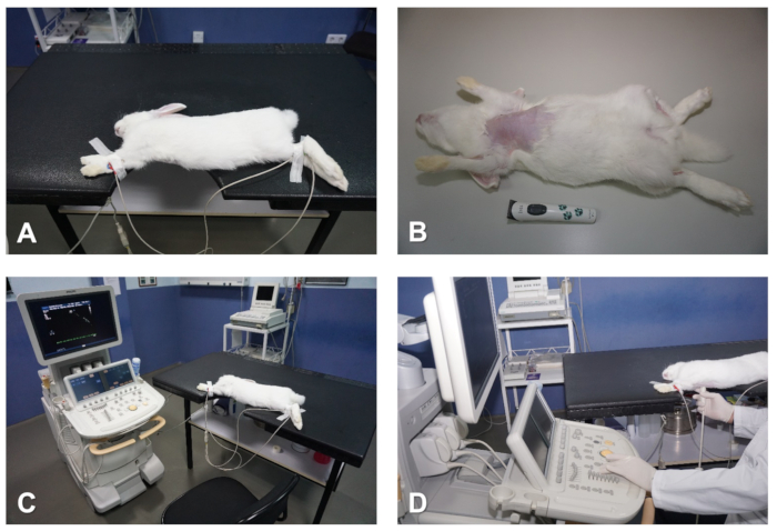
Figure 1. Preparation and positioning of the rabbit for echocardiography. (A) Table with notch that coincides with the cardiac area to be imaged. (B) Remove hair from the chest. (C) Attach ECG electrodes to monitor the heart. (D) Positioning of the operator whilst preforming echocardiographic examination. Please click here to view a larger version of this figure.

2. Parasternal long axis (sagittal) view of the heart

1. To obtain a parsternal long axis (PSLAX) view of the heart, place the rabbit in the right lateral recumbent position, with the forelimbs outstretched away from the thorax, with surgical tape (Figure 1A and Figure 1C).
   1. To achieve the best imaging quality possible, it is important to keep the skin of the thoracic region as flat as possible to increase the penetration and improve overall imaging quality whilst imaging the animal. For this, hold the forelimbs away from the thorax with one hand, whilst using the free hand to identify any skin folds and pockets, flatten these from top to bottom, and move any skin folding away from the chest towards the lateral side and back of the rabbit. This is particularly important for older and larger rabbits whose excessive skin and subcutaneous fat tissue could reduce image quality.
      NOTE: The cardiac area of the chest should be positioned over the cutout section in the table. However, keep in mind that, in this position, the abdomen has a natural tendency to move towards the notch, and creates a positive pressure that displaces the heart cranially, which then interferes with good echocardiographic imaging. To prevent this, it is important that the abdomen rests completely on the table and, to achieve this, it is useful to gently move the abdominal organs towards the caudal region of the animal through gentle massaging (Figure 1A and Figure 1C).
2. For echocardiographic imaging, hold the transducer with the right hand, whilst using the left hand to operate the controls of the echocardiography system as shown in Figure 1D.
   1. To maintain good skin contact, apply undiluted ethanol to the skin and then enough ultrasound transmission gel to the head of the transducer.
3. Next, position the transducer closely to the skin of the right hemithorax, at the level of the second to third intercostal space and about 1-3 cm away from the right parasternal line, with the transducer orientation mark pointing to the right shoulder of the animal and at an angle of approximately 30° relative to the midline (Figure 2A). This should produce an image of the right PSLAX of the heart (see Representative Results).
4. Once the 2D cardiac images are displayed on the screen, the next step is to adjust the ultrasound unit controls to obtain optimal images. The main ones are:
   1. Depth and zoom controls: Use these controls to optimize the area of interest. The depth of the image must be adequate so that the cardiac structures can be seen on each image. Use the zoom tool for better assessment of structures of interest, e.g., integrity of valves and leaflets.
   2. Total gain and time-gain compensation (i.e., gain settings at different depths in real time): Control gray scales and gains manually to minimize background noise and to maximize the delineation of cardiac structures. These parameters are especially important in rabbits because of the poor echogenicity of the ventricular myocardium.
   3. Dynamic range or compression: Use this control to adjust the number of shades of gray that are displayed by the image. Set the dynamic range so the blood pool is dark and the tissue is bright. This will result in better endocardial border definition, which is important to obtain left ventricular volumes.
   4. Sector width: Begin the examination with a wide sector (90°) and after an overview of the heart, reduce the sector width if specific areas need to be better imaged. Decreasing the sector size improves the temporal resolution by increasing the frame rate. This is especially important when 2D echocardiography is used to guide Doppler examination.
5. To maintain the position of the transducer whilst imaging the rabbit, and to reduce the fatigue of the operator, use the index finger to anchor the hand to the table or the chest of the animal, whilst the other fingers hold the transducer (Figure 2A).
6. Obtain two main imaging planes of the heart in the right PSLAX view.
   1. Find an imaging plane which sections the heart longitudinally and where all four chambers of the heart (two atria and two ventricles) can be identified; also, when a wide field of view is used, the apex of the heart should also come into view on the left side of the image (see Representative Results section).
   2. Perform subtle movements of the transducer, such as sweeping, rocking and rotation, relative to the intercostal space as well as the craniocaudal and dorsoventral angle of the ultrasound beam to obtain the other imaging plane of the parasternal long axis view (Figure 2A,B). In the other imaging plane, the left ventricular outflow track (LVOT) and the aorta can be identified (see Representative Results).
7. Image orientation: Note that the base of the heart will be on the right side of the sector image.
8. After obtaining the appropriate imaging planes, use B-mode to evaluate overall function of the heart, and use color Doppler to assess blood flow across all valves as well as the integrity of the interventricular septum (IVS).
   ​NOTE: Always save images of the different views and planes for offline analysis.

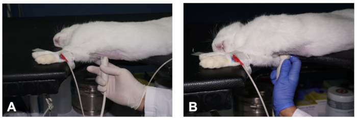
Figure 2. How to obtain a PSLAX view of the heart. (A- B) Positioning of the transducer to obtain the two different planes of the PSLAX view of the heart (see description in the text). Please click here to view a larger version of this figure.

3. Parasternal short axis view of the heart

1. With the transducer at the same location in the chest while displaying a well-aligned PSLAX, perform a counter clockwise rotation of the transducer of approximately 90° (Figure 3A) to obtain a right parasternal short axis (PSSAX) view. This time, the transducer orientation mark should be pointing towards the left shoulder of the rabbit.
   NOTE: To help maintain the transducer in the same location of the chest whilst rotating the transducer, use the left hand to perform the rotation from the cord of the transducer as shown in Figure 3B.
2. In the parasternal short axis view, obtain three imaging planes by sweeping the transducer along the axis of the heart: the mid-ventricular, the mitral valve, and the high base with the pulmonary artery (PA) and the aortic valve (AoV) in view.
   1. In the mid-ventricular imaging plane, which sections the heart at the papillary muscles and chordae tendineae level (Figures 3C), visualize the right ventricle (RV) at the top and the left ventricle (LV) at the bottom of the image (see Representative Results).
   2. Use B-mode to evaluate radial and circumferential contraction and relaxation of the LV, and check for regional wall motion abnormalities.
   3. Use M-mode and with the help of the track ball move the cursor in real time over the 2D image, and then place the cursor in the middle of the LV, between both papillary muscles, perpendicular to the IVS and left ventricular free wall (FW) (Figure 3C). Once the M-mode images are displayed on screen, store images for offline analysis. In rabbits with high heart rates, use higher sweep speeds to better separate cardiac events during the cardiac cycle (e.g., 150 mm/sec).
   4. By sweeping the transducer towards the cephalic region (Figure 3D), obtain a mitral valve (MV) plane. Use B-mode and M-mode to evaluate the integrity and motility of the MV leaflets. Place the cursor along the middle of the LV, perpendicular to the IVS (Figure 3E), to obtain detailed information regarding excursion of the MV in relation to the IVS.
   5. Sweep the transducer further cranially to result in an imaging plane at the level of the high base (also known as AoV plane; Figure 3F - H), where the AoV and its leaflets, the right ventricular outflow track (RVOT), the PA, and the right and left atria (LA) can be identified (see Representative Results).
   6. Image orientation: Note that the PA will be on the right side of the sector image.
   7. To completely visualize the PA and its bifurcation, use a greater angulation and, sometimes, a cranial displacement of the transducer (an intercostal space).
   8. Use B-mode for evaluation of the size and shape of these structures (e.g., left atrial size is increased in congestive heart failure), and use color Doppler and PWD to record the velocity of blood flow (outflow) at the PV level, by placing the sample volume just below the opening of the PV leaflets (Figure 3G). Finally, use M-mode and place the cursor along the AoV and LA (Figure 3H).
3. Use the following main controls and adjustments to obtain adequate color flow Doppler images:
   1. With the color sector positioned in the area of interest, reduce the angle between the sector and the blood flow direction as much as possible.
   2. Color sector width: Adjust this to the valve area, in order to increase the frame rate and improve the color flow information.
   3. Baseline and pulse repetition frequency (PRF): Adjust the baseline on the color bar and the PRF, to allow higher velocities to be displayed. A number at the top and bottom of the color bar represents the maximum detectable velocity before color aliasing occurs.
      NOTE: Aliasing is more frequent in color flow processingthan spectral pulsed Doppler, because a portion of the pulses is assigned to obtain cross sectional images in detriment to the color flow Doppler information.
   4. Color gain: First, increase this to the point that it just begins to create background noise, and then decrease to a level that optimizes color flow imaging.
4. Use the following main controls to obtain adequate spectral Doppler images:
   1. Cursor position: Make this parallel to blood flow direction; at least, maintain at an angle < 30°.
   2. Gate position: It is a marker in the cursor line corresponding to the sampling site. Place it after the aortic and pulmonary valves and at the leaflet tips of the atrioventricular valves.
   3. Gate size: Use the minimum setting except to obtain small regurgitant flows.
   4. Baseline: Select the baseline depending on the direction of the blood flow. Place it at the top when blood flows against the transducer (e.g. pulmonary and aortic flows), or at the bottom when the blood flows toward the transducer (e.g. atrioventricular valves flows).
   5. Scale: Select this according to the velocity of the blood flow, usually, 25% higher than the obtained velocity.
   6. Doppler gain: Use this to intensify the Doppler signals. Increase gain until the color displays.
   7. Colorization of the Doppler signal: Use magenta color when the Doppler spectrum is weak because it makes the velocity sharper.
   8. Wall filter: Use this to decrease the amount of low-frequency noise that is produced by the cardiac walls.
   9. Sweep speed: Use higher sweep speeds to facilitate time measurements.

Figure 3. How to obtain a PSSAX view and its different imaging planes. (A) Position of the transducer to obtain a PSSAX view at the level of the papillary muscles. (B) Demonstration of the role of the left hand to help in rotating the transducer when switching from a PSLAX to a PSSAX view. (C) Location of the cursor of M-mode in the papillary muscles plane of the PSSAX view. (D) Position of the transducer to obtain a PSSAX view of the heart at the mitral valve plane. (E) Location of the cursor of the M-mode in the MV plane of the PSSAX view. (F) Position of the transducer to obtain the AV plane in the PSSAX view. (G) Demonstration of color Doppler and positioning of the PWD sample volume to evaluate the outflow of the PV. (H) Location of the cursor of the M-Mode in the AoV plane of the PSSAX view. LV = Left ventricle; RV = right ventricle; FW = LV free wall; AoV = aortic valve; RVOT = right ventricular outflow track; PV = pulmonary valve; PA = pulmonary artery; LA = Left atrium; RA = right atrium. Please click here to view a larger version of this figure.

4. Apical 4 chambers view of the heart

1. To obtain an Apical 4 chambers (AP4C) view, place the rabbit in the left lateral recumbent position with the forelimbs outstretched away from the thoracic region by means of surgical tape ( Figure 4A). Maintain the skin of the thorax flat in a similar way as described above (Step 2.1.1). The cardiac area of the chest should be positioned over the cutout section of the table. Similarly, the abdomen should be well-supported on the table after moving caudally the abdominal organs through gentle massaging.
2. Apply ultrasound gel to the transducer, and then access the heart through the notch in the table and position it closely to the skin of the left hemithorax, at the level of the 4^th-5^th intercostal space with the midclavicular line, with the transducer orientation mark pointing towards the back of the rabbit (in the direction of the left scapula) (Figure 4B). In this way, the transducer is orthogonal with the apex of the heart and the ultrasound beam is directed towards the base of the heart.
   1. From this position, if necessary, move the transducer upward one intercostal space at a time until the ~4th intercostal space (a maneuver often called "window shopping").
   2. Upon reaching the appropriate intercostal space (which may vary according to size and/or age of the rabbit), observe an image of the heart from the apex to the base of the heart, the typical heart shape where all four chambers can be seen, with the left and right ventricles at the top and both atria at the bottom of the image (see Figure 4C,D and Representative Results).
   3. Image orientation: Note that the LV will be on the right side of the sector image.
3. Avoid foreshortening the apex in this view, so that the typical AP4C view of the heart should give a bullet shape image of the LV with the IVS in the middle (Figure 4C,D). If the apex is rounded, the LV is likely foreshortened; therefore, move the transducer downwards one intercostal space and/or tilt of the transducer.
   1. Use B-mode to check for regional wall motion abnormalities and have a global view of the LV function. Use color Doppler to evaluate flow across the atrioventricular valves, and use PWD and position the sample volume at the level of the MV leaflet tips to obtain images of the MV inflow spectrum (Figure 4C).
   2. Use TDI mode and place the sample volume at the septal and lateral sides of the mitral valve annulus (Figure 4D).
   3. Use M-mode and place the cursor aligned with the lateral MV annulus to obtain the mitral annular plane systolic excursion (MAPSE). Store images in each of these modes for offline analysis of cardiac function.

Figure 4. How to obtain the AP4C and AP5C views of the heart. (A) Positioning of the rabbit in left lateral decubitus for an AP4C view of the heart. (B) Position of the transducer to obtain an AP4C view of the heart. (C) Location of the sample volume at the MV leaflet tips to evaluate MV inflow. (D) Location of the sample volume for TDI analysis of myocardial velocities at the lateral side of the MV annulus. (E) Position of the transducer to obtain an AP5C view of the heart. (F) Location of the sample volume for PWD analysis of the outflow across the AoV. LV = Left ventricle; RV = right ventricle; MV = mitral valve; LA = left atrium; RA = right atrium; AoV= Aortic valve. Please click here to view a larger version of this figure.

5. Apical 5 chambers view of the heart

1. Starting with the transducer at the same location as in AP4C view, perform a gentle tilting caudally (Figure 4E) until the LVOT and AoV come into view, this is the apical 5 chambers view (AP5C) of the heart (see Representative Results).
2. Use B-mode to evaluate the LVOT, the movement of the AoV leaflets, as well as the LV cavity size and function.
3. Use color Doppler mode for evaluation of outflow across the AoV, and use PWD to assess flow velocity across this valve by positioning the sample volume just behind the AoV (Figure 4F).

Results

Parasternal long axis view of the heart

Figure 5A shows an imaging plane of the right PSLAX view where the 4 chambers of the heart are clearly distinguished. You can identify in this view the right ventricle (RV), tricuspid valve (TV), IVS, LV, FW, as well as the mitral valve (MV). When the apex is clearly visible on the left side of the image in this view and the LV is not foreshortened, it is possible to estimate accurately the LV volume using the biplane method of disks (modified Simpson's rule) as shown in Figure 5B,C⁸, which for accuracy should be combined with a similar measurement of the LV volume in the AP4C view, especially if the rabbit model used presents with wall motion abnormalities. Figure 5D shows the other imaging plane of the right PSLAX where the LVOT and the Aorta (Ao) also come into view. The location for placement of the calipers for accurate measurement of the LVOT is also shown in Figure 5D. 

Figure 5. Imaging planes obtained in a PSLAX view of the heart. (A) Imaging plane demonstrating the 4 chambers of the heart. (B) End diastolic and (C) end systolic images, demonstrating Simpson's method for analysis of the LV. (D) Imaging plane where the LVOT and aorta come into view in the PSLAX view of the heart. LV = Left ventricle; RV = right ventricle; IVS = interventricular septum; Ao = aorta; LVOT = left ventricular outflow track; LA = Left atrium; RA = right atrium; MV = mitral valve; TV = tricuspid valve; FW = free wall of the LV; PC = pericardium. Please click here to view a larger version of this figure.

Parasternal short axis view of the heart

In Figure 6A, a right PSSAX view of the heart at the level of the papillary muscles and chordae tendineae plane is shown. It is possible identify in this view the RV, IVS, LV, and FW, as well as the anterolateral (AL) and posteromedial (PM) papillary muscles (Figure 6A). In this view, the area trace tool is used to measure the circumferential area in end-diastole (CAd) (Figure 6B), and in end-systole (CAs) (Figure 6C), which allows the calculation of the total circumferential shortening area (CSA) by using the formula:

CSA=CAd-CAs/CAd×100.

An example of an M-mode trace in the PSSAX at the papillary muscles level is shown in Figure 6D, where the placement of calipers, leading edge to leading edge, for the different measurements of the structures of the LV is also demonstrated. These measurements provide useful information regarding size of the LV structures. Thus, measuring the LV end-diastolic diameter (LVDd) and LV end-systolic diameter (LVDs) from three consecutive heart beats allows the calculation of the LV shortening fraction (%SF), using the formula:

SF%= LVDd-LVDs/LVDd

as well as the LV systolic and diastolic volumes (LVVd, LVVs), using the Teichholz formula:

(7×(LVD)³)/(2.4+LVD)

The LV ejection fraction (LVEF (%)) is subsequently calculated according the formula LVEF=(LVVd-LVVs)/(LVVd×100).

An M-mode trace at the level of the MV plane in PSSAX view is shown in Figure 6E, where the location of the calipers for measurement of the E-point to septal separation (EPSS) of the mitral valve is also shown. An example of a PSSAX view of the heart at the AoV plane level is shown in Figure 6F, where the location of the calipers for measurement of the Aortic root diameter (AoD), as well as the left atrial dimension (LAD) are demonstrated.

An example of the PV outflow analysis using both color Doppler and pulsed wave Doppler is shown in Figure 6G. Note the blue colored outflow through the PV with color Doppler, which indicates that the flow observed is moving away from the transducer. Examples of how to quantitate the pre-ejection period of the PV (PEP PV), as well as the PV outflow using the volume time integral (VTI), are shown in Figure 6H.

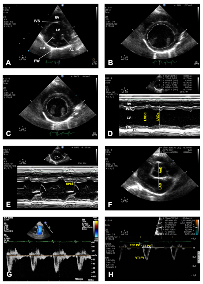
Figure 6. Imaging planes obtained in the PSSAX view. (A) Representative image of a PSSAX view at the papillary muscles plane. (B) End diastolic and (C) end systolic tracing of the endocardial border to measure the total CSA. (D) M-mode trace obtained in a PSSAX view at the level of the papillary muscles. (E) An example of M-mode trace obtained in a PSSAX view at the level of the MV. (F) Representative 2D image of a PSSAX vie in the plane of the AV. (G) Color Doppler-guided PWD tracing of the PV outflow. (H) Demonstration of a VTI tracing using the PWD signal obtained from the PV outflow. LV = Left ventricle; RV = right ventricle; IVS = interventricular septum; FW = free wall of the LV; AL = anterolateral papillary muscle; PM = posteromedial papillary muscle; LVDd = left ventricular diameter at end-diastole; LVDs = left ventricular diameter at end-systole; PC = pericardium; EPSS = E-point to septal separation; AoD = aortic root diameter; LAD = left atrial dimension; MV = mitral valve; TV = tricuspid valve; PEP PV = pre-ejection period of the pulmonary valve; ET PV = ejection time of the pulmonary valve; VTI PV = volume time integral of the pulmonary valve. Please click here to view a larger version of this figure.

Apical 4 chambers view

An example of MV inflow using color Doppler in an AP4C view is shown in Figure 7A. Note the predominant red color of the MV inflow indicating that the flow is moving towards the transducer. Thus, a useful mnemonic to describe and learn how blood flows across the structures of the heart is the acronym BART (Blue Away, Red Towards the transducer). Using PWD, the MV inflow spectrum can be assessed as shown in Figure 7B, where the early (E) and late (A) filling waves during diastole are easily differentiated. Examples of myocardial tissue velocities of the MV annulus as assessed by TDI at both the lateral and septal walls are shown in Figure 7C and Figure 7D, respectively. The systolic component is denoted by the S wave, whilst the E' and A' waves correspond with myocardial movement of the mitral valve annulus during early filling (E') and late filling (A') components of diastole.

Apical 5 chambers view

Figure 7E shows an example of color Doppler positioned at the LVOT in an apical 5 chambers view. Note that, in line with the BART mnemonic described above, the blue color observed indicates that blood flow is moving away from the transducer. Figure 7F shows an example of how to quantitate the AoV outflow using PWD signal to evaluate the VTI of the AoV, systolic ejection time (ET) and pre-ejection period of the AoV (PEP AoV).

Figure 7. The AP4C and AP5C views. (A) An example of color Doppler in an AP4C view. (B) Representative image of the PWD signal of the MV inflow in an AP4C, where E wave corresponds with early diastolic filling and A corresponds with atrial contraction component during diastole. (C-D) Representative images of myocardial velocity signals obtained from the lateral (C) and septal (D) segments of the MV annulus using TDI in an AP4C view. S corresponds with systole, whilst E' corresponds with early filling phase and A' with late filling phase during diastole. (E) An example of color Doppler signal obtained from the AoV in an AP5C view. (F) Demonstration of a VTI tracing using the PWD signal obtained from the AoV outflow. AoV = Aortic valve; VTI = volume time integral; PEP = pre-ejection period; ET = ejection time. Please click here to view a larger version of this figure.

Discussion

We have described a protocol for the echocardiographic examination of cardiac function parameters in the rabbit, representing a large preclinical model^1,2,3. The step by step methodology described herein should be considered guidance, which with a complementary study of the basic principles of echocardiography, and a basic knowledge of ultrasound imaging, will help the researcher to obtain, through practice and complementary and expert guidance, good quality data in a relative short period of time.

There are several critical steps to increase the value and reproducibility of the results whilst using the echocardiography protocol described here. First, ensure the skin of the thorax is hair free and clean; for this we recommend cleaning the skin with ethanol to remove excess of natural skin grease before applying ultrasound gel. Next, whilst it is possible to image the chest in a supine position, the lungs tend to inflate and reduce an already difficult to image chest wall with poor echogenicity, thus, a left or right recumbent position of the rabbit and the application of the transducer to the chest through the cut-out notch of a purpose built imaging table is the best way to improve overall imaging quality. Then, the researcher operating the ultrasound system should spend some time creating cardiac imaging presets with optimized imaging settings, which are essential to improve overall imaging quality in all views and will also shorten your imaging time at future imaging sessions. Some of the most important control settings to master are total gain and time-gain compensation, given the poor imaging of the chest of the rabbit (see step 2.4.2). It is also important to be systematic and always perform the echocardiographic examination in an orderly fashion. For this, getting into the habit of acquiring all the imaging views and imaging planes in the same sequence will avoid missing important information whilst performing the study. Furthermore, during imaging analysis it is recommended to perform all measurements in at least three consecutive cardiac cycles in the acquired images for each modality. Finally, the blinding of the observer during imaging as well as during the offline analysis is important to avoid bias and increase the value of the results for translational medicine. Taking into account all of the above considerations, together with the application of the principles of imaging and analysis according to current guidelines^7,8, will ensure the reproducibility of the research using longitudinal evaluation of cardiac function via echocardiography in a large animal model such as the rabbit.

Given the variability in body size and fat composition at different ages of the rabbits and the particular experimental settings, some variations of the technique will be required, such as subtle movements of the transducer (e.g., sweeping, rotation) relative to the intercostal space, in order to achieve the desired imaging planes. Therefore, the protocol described here must be interpreted as a starting point that should be adapted to the particular objectives of the research program involving this technique.

Whilst clinical echocardiography systems are widely available in most research centers, there are some limitations to the technique described herein. Indeed, the quality of the images obtained from echocardiographic studies depends to a large extent on the sophistication and technology of the ultrasound machine, the skills and expertise of the operator, and the individual patient characteristics. The minimum technical characteristics that the ultrasound equipment must meet were described in the introduction. Thus, inadequate equipment (e.g., a linear array transducer) constitutes a fundamental limitation for the use of the echocardiographic technique in the rabbit model. In addition, the echocardiographic technique and its results are strongly influenced by the operator. Therefore, an operator without enough experience and practical training could dramatically limit the obtaining of standardized images of appropriate quality. Similarly, inexperienced operators could also make mistakes in obtaining measurements even if they are performed on echocardiographic images of excellent technical quality. Furthermore, as mentioned above, some of the limitations are inherent to the rabbit model, such as age and, more specifically, by the size and body fat composition of the rabbits studied via echocardiography. In our experience, young rabbits weighing up to 2.5 kg have low subcutaneous and intra-thoracic fatty deposits. This phenotypic stage provides the best acoustic windows and offers crisper and sharper echocardiographic images and very few artefacts. As the size and body fat composition increase, the quality and accuracy of the echocardiographic study becomes limited, and the skills of the operator will ultimately play a fundamental role in achieving the best possible imaging under these circumstances.

We currently use echocardiography for longitudinal evaluation of cardiac function in a rabbit model of cardiomyopathy induced by anthracyclines and to test stem cell therapies for this condition^9,12,13. The technique described here could also be used in other preclinical studies involving ischemia or valvular heart disease.

Another cardiovascular imaging technique is cardiac magnetic resonance (CMR), whose main advantage is better endocardial-myocardial definition, which translates into a more accurate estimation of LV volumes and systolic function¹⁴. However, CMR is limited by its high cost and lack of portability and therefore its limited availability in most research centers. Similarly, CMR has relative poor performance for the analysis of diastolic function, thus making echocardiography a better overall choice for longitudinal evaluation of systolic and diastolic function of the heart¹⁵.

In our experience, the anesthetic regime used in the protocol described herein is safe and achieves reproducible results without significant depression of myocardial function attributable to the anesthesia⁹. However, it is important to standardize the anesthetic regime in each laboratory to ensure reproducible results for your particular experimental settings. After inducing anesthesia, in experienced hands the echocardiographic examination can be completed within 15 min.

Materials

List of materials used in this article

Name	Company	Catalog Number	Comments
Bluesensor	Medicotest	13BY1062	Disposable adhesive ECG lectrodes
Domtor (Medetomidine)	Esteve	CN 570686.3	Veterinary prescription is necessary
HD11 XE Ultrasound System	Philips	10670267	Echocardiography system.
Heating Pad	Solac	CT8632
Imalgene (Ketamine)	Merial	RN 9767	Veterinary prescription is necessary
Omnifix-F 1 ml syringe	Braun	9161406V
S12-4	Philips	B01YgG	4-12 MHz phase array transducer
Ultrasound Transmision Gel (Aquasone)	Parker laboratories Inc.	N 01-08

References

- Pogwizd, S. M., Bers, D. M. Rabbit models of heart disease. Drug Discovery Today Disease Models. 5, 185-193 (2008).
- Gandolfi, F., et al. Large animal models for cardiac stem cell therapies. Theriogenology. 75, 1416-1425 (2011).
- Harding, J., Roberts, R. M., Mirochnitchenko, O. Large animal models for stem cell therapy. Stem Cell Research & Therapy. 4, 23(2013).
- Chong, J. J., Murry, C. E. Cardiac regeneration using pluripotent stem cells--progression to large animal models. Stem Cell Research. 13, 654-665 (2014).
- Del, M. F., Mynett, J. R., Sugden, P. H., Poole-Wilson, P. A., Harding, S. E. Subcellular mechanism of the species difference in the contractile response of ventricular myocytes to endothelin-1. Cardioscience. 4, 185-191 (1993).
- Sahn, D. J., DeMaria, A., Kisslo, J., Weyman, A. Recommendations regarding quantitation in M-mode echocardiography: results of a survey of echocardiographic measurements. Circulation. 58, 1072-1083 (1978).
- Thomas, W. P., et al. Recommendations for standards in transthoracic two-dimensional echocardiography in the dog and cat. Echocardiography Committee of the Specialty of Cardiology, American College of Veterinary Internal Medicine. Journal of Veterinary Internal Medicine. 7, 247-252 (1993).
- Lang, R. M., et al. Recommendations for cardiac chamber quantification by echocardiography in adults: an update from the American Society of Echocardiography and the European Association of Cardiovascular Imaging. European Heart Journal Cardiovascular Imaging. 16, 233-270 (2015).
- Talavera, J., et al. An Upgrade on the Rabbit Model of Anthracycline-Induced Cardiomyopathy: Shorter Protocol, Reduced Mortality, and Higher Incidence of Overt Dilated Cardiomyopathy. BioMed Research International. 2015, 465342(2015).
- Borkowski, R., Karas, A. Z. Sedation and anesthesia of pet rabbits. Clinical Techniques in Small Animal Practice. 14, 44-49 (1999).
- Cantwell, S. L. Ferret, rabbit and rodent anesthesia. The Veterinary Clinics of North America. Exotic Animal Practice. 4, 169-191 (2001).
- Giraldo, A., et al. Percutaneous intramyocardial injection of amniotic membrane-derived mesenchymal stem cells improves ventricular function and survival in non-ischaemic cardiomyopathy in rabbits. European Heart Journal. 36, 149(2015).
- Giraldo, A., et al. Allogeneic amniotic membrane-derived mesenchymal stem cell therapy is cardioprotective, restores myocardial function, and improves survival in a model of anthracycline-induced cardiomyopathy. European Journal of Heart Failure. 19, 594(2017).
- Bellenger, N. G., et al. Comparison of left ventricular ejection fraction and volumes in heart failure by echocardiography, radionuclide ventriculography and cardiovascular magnetic resonance; are they interchangeable? European Heart Journal. 21, 1387-1396 (2000).
- Flachskampf, F. A., et al. Cardiac Imaging to Evaluate Left Ventricular Diastolic Function. Journal of the American College of Cardiology Cardiovascular Imaging. 8, 1071-1093 (2015).
Reprints and Permissions