A Plasma Sample Preparation for Mass Spectrometry using an Automated Workstation

Summary

Here, we present an automated plasma protein digestion method for mass spectrometry-based quantitative proteomic analysis. In this protocol, the liquid transferring and incubation steps for protein denaturation, reduction, alkylation, and trypsin digestion reactions are streamlined and automated. It takes approximately five hours to prepare a 96-well plate with desired precision.

Abstract

Sample preparation for mass spectrometry analysis in proteomics requires enzymatic cleavage of proteins into a peptide mixture. This process involves numerous incubation and liquid transfer steps in order to achieve denaturation, reduction, alkylation, and cleavage. Adapting this workflow onto an automated workstation can increase efficiency and reduce coefficients of variance, thereby providing more reliable data for statistical comparisons between sample types. We previously described an automated proteomic sample preparation workflow¹. Here, we report the development of a more efficient and better controlled workflow with the following advantages: 1) The number of liquid transfer steps is reduced from nine to six by combining reagents; 2) Pipetting time is reduced by selective tip pipetting using a 96-position pipetting head with multiple channels; 3) Potential throughput is increased by the availability of up to 45 deck positions; 4) Complete enclosure of the system provides improved temperature and environmental control and reduces the potential for contamination of samples or reagents; and 5) The addition of stable isotope labeled peptides, as well as β-galactosidase protein, to each sample makes monitoring and quality control possible throughout the entire process. These hardware and process improvements provide good reproducibility and improve intra-assay and inter-assay precision (CV of less than 20%) for LC-MS based protein and peptide quantification. The entire workflow for digesting 96 samples in a 96-well plate can be completed in approximately 5 hours.

Introduction

Mass spectrometry (MS) -based protein and peptide quantification is increasingly being applied as a bioanalytical tool for plasma analysis in basic research and clinical laboratories^2,3. The requisite instrumentation and informatics have advanced rapidly as MS has become the method of choice for quantifying proteins or modified proteins by targeting specific peptide sequences due to its ability to quantify hundreds of peptides in a single MS run⁴. Sample preparation serves as the foundation for any proteomic analysis. Prior to MS analysis, the proteins in a biological sample are typically denatured, reduced, alkylated, digested into tryptic peptides, and desalted⁵. Alkylation blocks cysteines to prevent uncontrolled modifications and ensure all cysteines have the same mass. Next, trypsin is added to digest proteins into peptides. Each of these steps requires optimization, and the entire process is traditionally performed manually, allowing for the introduction of analytical errors.

The traditional biomarker development pipeline consists of two main processes: shotgun proteomics for global protein discovery to create an in-depth protein inventory⁶ and targeted proteomics for verification and validation aimed at high-precision and high-throughput protein quantitation⁷. Regardless of the MS approach, sample preparation is the same and centers on enzymatic cleavage of proteins into a peptide mixture. As proposed by Van Eyk and Sobhani⁸, having a method that allows for accurate, precise, and reproducible analysis for both discovery and targeted assays is desired to effectively move discovery biomarkers to clinical implemented assays. To do this, automation of sample preparation will be helpful and provide the ability to increase the efficiency to high-throughput analysis. Manual methods typically introduce analytical errors beyond acceptable limits specified by the Food and Drug Administration (FDA) in the revised Bioanalytical Method Validation Guidance, which includes biomarkers and diagnostics^2,9. The development of a fast, highly accurate, and hands-free MS protein sample preparation workflow will be necessary to facilitate biomarker research, which requires preparing and analyzing thousands of biological samples. MS sample preparation has many steps where errors can be introduced, and the process is tedious and time-consuming.

In our improved method, an automated workstation was programed to perform all necessary plasma sample preparation procedures in a total of 6 steps (Figure 1) to ensure: 1) accurate liquid transfers; 2) the reaction is initiated and stopped at a consistent time; 3) the reaction is performed at a controlled temperature (i.e., incubator); and 4) the reaction has uniform mixing for all reactions. We also implemented adding exogenous quality control proteins and internal standards (stable isotope-labeled peptide standards) to ensure a quality and reproducible throughput of LC-MS-based protein and peptide quantification in a 96-well format. Including reagent preparation, hours of work time and a total of 1,000,000 pipetting steps would be required to process 96 samples in individual tubes. Automation reduces the hands-on time and the number of human interactions involved.

Protocol

1. Programing for the automated liquid handler

1. Create a new method from File menu (File | New Method)
   NOTE: Complete the steps in the order given. The italic font denotes text to type in the Biomek software. Please contact the authors for information regarding pipetting techniques and templates.
2. Type Start step variables and their values in the start step as listed in Table 1.
3. Set columns for selective tip pipetting. For the steps 1.3-1.7, click the Set Global step in the toolbar under Control Steps and drag it to the method.
   1. Using the Set Global step, set value =FirstColumn to variable FirstColumn_Global, value =LastColumn to variable LastColumn_Global, value =LastColumn-FirstColumn+1 to variable Columns, and value =Columns*8 to variable Wells.
   2. Select the Script step in the toolbar under Control Steps and drag it to the method. Type the VB script as indicated in Figure 2.
4. Setting volumes for mixes Set Global and solutions.
   1. Using the Set Global step, set the corresponding values to the volume mix variables as shown in Table 2.
   2. Click the If step in the toolbar under Control Steps and drag it to the method. Under conditions, type Autosampler.
   3. Under Then, click the Set Global step in the toolbar under Control Steps and drag it to the method.
   4. Using the Set Global step, set value =(MobilePhase*Columns)+10 to variable MobilePhaseWell.
   5. Under Else, click the Set Global step in the toolbar under Control Steps and drag it to the method.
   6. Using the Set Global step, set value =0 to variable MobilePhaseWell
5. Configuring Guided Labware Setup (GLS)
   1. Click the Deck Editor step in the toolbar under Utilities. Create a new deck to correspond with the deck layout in Figure 3 and label it as Deck 1.
   2. Click the Guided Setup step in the toolbar under Setup & Devices and drag it to the method. Drag and drop the labware types in the deck positions as indicated in Table 3. Thereafter, fill the tabs in the table as shown in Table 3 and Figure 4 (Setting up the Guided Setup).
6. Setting up procedure for tip counting
   1. Click the Define Procedure step in the toolbar under Control Steps and drag it to the method. Name procedure as TipCount.
   2. Click the Script step in the toolbar under Control Steps and drag it to the method. Type the VB script as indicated in Figure 5 (Tip counting script).
   3. Click the If step in the toolbar under Control Steps and drag it to the method.
   4. Under conditions, type TL5 = 0.
   5. Under Then, click the Move Labware step in the toolbar under Setup & Device Steps and drag it to the method. Move labware from TL5 to TR3. Click the Move Labware step in the toolbar, under Setup & Device Steps and drag it to the method. Move labware from TL2 to TL5. Finally, click the Move Labware step in the toolbar under Setup & Device Steps and drag it to the method. Move labware from BC90 to TL2.
7. Defining procedure for incubator
   1. Click the Define Procedure step in the toolbar under Control Steps and drag it to the method. Name procedure as Incubator.
   2. Type in HalfTime as Variable Name and 1800 as Default Value.
   3. Type in NextTemp as Variable Name and 22 as Default Value.
   4. Type in temp as Variable Name and 60 as Default Value.
   5. Click the Enhanced Move Labware step in the toolbar under Setup & Device Steps and drag it to the method. Move labware from P11 to INHECO1.
   6. Click the Run Procedure step in the toolbar under Control Steps and drag it to the method. Name procedure as TipCount.
   7. Click the INHECO Incubate step in the toolbar under Integrations and drag it to the method. Type in INHECO1 for use the device at position, =HalfTime for Incubate for, =Temp for °C and 3 for °C of target temperature. Select the Shake while incubating option and Orbital (clockwise) shake style. For settings, type in 1.00 mm side to side, 6.6 times a second, 1.00 mm forwards ad backwards and 6.6 times a second.
      NOTE: Make sure INHECO Incubator software is installed.
   8. Click the INHECO Incubate step in the toolbar under Integrations and drag it to the method. Type in INHECO1 for use the device at position, =HalfTime for Incubate for, =Temp for °C and 3 for °C of target temperature. Select the Shake while incubating option and Orbital (Counter-clockwise) shake style. For settings, type in 1.00 mm side to side, 6.6 times a second, 1.00 mm forwards and backwards at 6.6 times a second.
   9. Click the Pause step in the toolbar under Setup & Device Steps and drag it to the method. Pause the whole system for 1 s.
   10. Click the Define Procedure step in the toolbar under Control Steps and drag it to the method. Name procedure as Incubator.
   11. Click the INHECO Incubate step in the toolbar under Integrations and drag it to the method. Type in INHECO1 for use the device at position, 1 for Incubate for, =NextTemp for °C and 3 for °C of target temperature.
8. Defining procedure for Orbital.
   1. Click the Enhanced Move Labware step in the toolbar under Setup & Device Steps and drag it to the method. Move labware from P11 to Orbital1.
   2. Click the Run Procedure step in the toolbar under Control Steps and drag it to the method. Select procedure TipCount.
   3. Click the Device Action step in the toolbar under Setup & Device Steps and drag it to the method. Select Device OritalShaker0, Command TimedShake. Enter Shaking speed 1000, Time to reach full speed 2, Time to shake 30.
   4. Click the Enhanced Move Labware step in the toolbar under Setup & Device Steps and drag it to the method. Move labware Orbital1 to P11.
9. Setting up the first mix
   1. Click the Select Tip step in the toolbar under Liquid Handling Steps and drag it to the method. Select rearrange position TL4.
   2. Click the INHECO Incubate step in the toolbar under Integrations and drag it to the method. Type in INHECO1 for use the device at position, 1 for Incubate for, 60 for °C and 3 for °C of target temperature.
   3. Click the Loop step in the toolbar under Control Steps and drag it to the method, within Select Tip step. Type col as variable =FirstColumn as Start, =LastColumn as End, and 1 as Increment.
   4. Click the Select Tips Load Tips step in the toolbar under Liquid Handling Steps and drag it to the method, within loop step. Select BC90 Tips, TL5 Location and TL2 backup Tips Location from the drop-down menu. Select Single Column(s) and type in 1.
   5. Click the Select Tips Aspirate step in the toolbar under Liquid Handling Steps and drag it to the method, within loop step. Select BCDeep96Round Labware Type and Reagent Plate Position. Type in volume =FirstMix, Aspirate at column 1 and row 1. Select an optimized technique from the technique drop-down menu.
   6. Click the Select Tips Dispense step in the toolbar under Liquid Handling Steps and drag it to the method, within loop step. Select BCDeep96Round Labware Type and Reagent Plate Position. Type in volume =FirstMix, dispense at column =col and row 1. Select an optimized technique from the technique drop-down menu.
   7. Click the Select Tips Unload step in the toolbar under Liquid Handling Steps and drag it to the method, within loop step. Select Unload tips to TR1.
10. Setting up the samples
    1. Click the If step in the toolbar under Control Steps and drag it to the method. Type SamplePlate as the condition.
    2. Under Then, click the Select Tips Load Tips step in the toolbar under Liquid Handling Steps and drag it to the method. Select BC90 Tips, TL5 Location and TL2 backup Tips Location from the drop-down menu. Select Single Column(s) and type in =tipcolumns.
    3. Click the Select Tips Aspirate step in the toolbar under Liquid Handling Steps and drag it to the method, within then. Select Greiner96RoundPS Labware Type and Samples Position. Type in volume =Sample, Aspirate at column =FirstColumn and row 1. Select an optimized technique from the technique drop-down menu.
    4. Click the Select Tips Dispense step in the toolbar under Liquid Handling Steps and drag it to the method, within then. Select BCDeep96Round Labware Type and Reaction Plate Position. Type in volume =Sample, dispense at column = FirstColumn and row 1. Select an optimized technique from the technique drop-down menu.
    5. Click the Select Tips Unload step in the toolbar under Liquid Handling Steps and drag it to the method, within then. Select Unload tips to TR1.
    6. After the end of the If step, click the Run Procedure step in the toolbar under Control Steps and drag it to the method. Select procedure Incubator. Type in HalfTime as Variable Name and 1800 as Default Value. Type in NextTemp as Variable Name and 22 as Default Value. Type in temp as Variable Name and 60 as Default Value.
11. Setting up the Cysteine Block
    1. Click the Loop step in the toolbar under Control Steps and drag it to the method, within Select tip step. Type col as variable =FirstColumn as Start, =LastColumn as End and 1 as Increment.
    2. Under Loop, click the Select Tips Load Tips step in the toolbar under Liquid Handling Steps and drag it to the method. Select BC90 Tips, TL5 Location and TL2 backup Tips Location from the drop-down menu. Select Single Column(s) and type in 1.
    3. Click the Select Tips Aspirate step in the toolbar under Liquid Handling Steps and drag it to the method, within the loop. Select BCDeep96Round Labware Type and Reagent Plate Position. Type in volume =CysteineMix, aspirate at column 2 and row 1. Select an optimized technique from the technique drop-down menu.
    4. Click the Select Tips Dispense step in the toolbar under Liquid Handling Steps and drag it to the method, within the loop. Select BCDeep96Round Labware Type and Reaction Plate Position. Type in volume = CysteineMix, dispense at column = col and row 1. Select an optimized technique from the technique drop-down menu.
    5. Click the Select Tips Unload step in the toolbar under Liquid Handling Steps and drag it to the method, within then. Select Unload tips to TR1.
    6. After the end of the If loop, click the Run Procedure step in the toolbar under Control Steps and drag it to the method. Select procedure Incubator. Type in HalfTime as Variable Name and 300 as Default Value. Type in NextTemp as Variable Name and 43 as Default Value. Type in temp as Variable Name and 25 as Default Value.
12. Setting up the second mix
    1. Click the Loop step in the toolbar under Control Steps and drag it to the method, within Select tip step. Type col as variable =FirstColumn as Start, =LastColumn as End and 1 as Increment.
    2. Under loop, click the Select Tips Load Tips step in the toolbar under Liquid Handling Steps and drag it to the method. Select BC90 Tips, TL5 Location and TL2 backup Tips Location from the drop-down menu. Select Single Column(s) and type in 1.
    3. Click the Select Tips Aspirate step in the toolbar under Liquid Handling Steps and drag it to the method, within the loop. Select BCDeep96Round Labware Type and Reagent Plate Position. Type in volume =SecondMix, Aspirate at column 3 and row 1. Select an optimized technique from the technique drop-down menu.
    4. Click the Select Tips Dispense step in the toolbar under Liquid Handling Steps and drag it to the method, within the loop. Select BCDeep96Round Labware Type and Reaction Plate Position. Type in volume = SecondMix, Dispense at column = col and row 1. Select an optimized technique from the technique drop-down menu.
    5. Click the Select Tips Unload step in the toolbar under Liquid Handling Steps and drag it to the method, within then. Select Unload tips to TR1.
    6. After the end of the If the loop, click the Run Procedure step in the toolbar under Control Steps and drag it to the method. Select procedure Orbital.
    7. Click the Pause step in the toolbar under Setup & Device Steps and drag it to the method. Pause the whole system for 1 s.
13. Setting up Trypsin addition
    1. Click the Loop step in the toolbar under Control Steps and drag it to the method, within Select tip step. Type col as variable =FirstColumn as Start, =LastColumn as End and 1 as Increment.
    2. Under Loop, click the Select Tips Load Tips step in the toolbar under Liquid Handling Steps and drag it to the method. Select BC90 Tips, TL5 Location, and TL2 backup Tips Location from the drop-down menu. Select Single Column(s) and type in 1.
    3. Click the Select Tips Aspirate step in the toolbar under Liquid Handling Steps and drag it to the method, within the loop. Select BCDeep96Round Labware Type and Reagent Plate Position. Type in volume =Trypsin, Aspirate at column 4 and row 1. Select an optimized technique from the technique drop-down menu.
    4. Click the Select Tips Dispense step in the toolbar under Liquid Handling Steps and drag it to the method within the loop. Select BCDeep96Round Labware Type and Reaction Plate Position. Type in volume =Trypsin, Dispense at column = col and row 1. Select an optimized technique from the technique drop-down menu.
    5. Click the Select Tips Unload step in the toolbar under Liquid Handling Steps and drag it to the method, within then. Select Unload tips to TR1.
    6. After the end of the If loop, click the Run Procedure step in the toolbar under Control Steps and drag it to the method. Select procedure Incubator. Type in HalfTime as Variable Name and 3600 as Default Value. Type in NextTemp as Variable Name and 25 as Default Value. Type in temp as Variable Name and 43 as Default Value.
    7. Click the INHECO Incubate step in the toolbar under Integrations and drag it to the method. Make sure INHECO Incubator software is installed. Type in INHECO1 for use the device at position, 1 for Incubate for, 25 for °C and 5 for °C of target temperature.
14. Setting up quenching
    1. Click the Loop step in the toolbar under Control Steps and drag it to the method, within Select Tip step. Type col as variable =FirstColumn as Start, =LastColumn as End and 1 as Increment.
    2. Under Loop, click the Select Tips Load Tips step in the toolbar under Liquid Handling Steps and drag it to the method. Select BC90 Tips, TL5 Location and TL2 backup Tips Location from the drop-down menu. Select Single Column(s) and type in 1.
    3. Click the Select Tips Aspirate step in the toolbar under Liquid Handling Steps and drag it to the method, within the loop. Select BCDeep96Round Labware Type and Reagent Plate Position. Type in volume =Quench, Aspirate at column 5 and row 1. Select an optimized technique from the technique drop-down menu.
    4. Click the Select Tips Dispense step in the toolbar under Liquid Handling Steps and drag it to the method, within the loop. Select BCDeep96Round Labware Type and Reaction Plate Position. Type in volume =Quench, Dispense at column = col and row 1. Select an optimized technique from the technique drop-down menu.
    5. Click the Select Tips Unload step in the toolbar under Liquid Handling Steps and drag it to the method, within Then. Select Unload tips to TR1.
    6. After the end of the If the loop, click the Run Procedure step in the toolbar under Control Steps and drag it to the method. Select procedure Orbital.
    7. Click the Pause step in the toolbar under Setup & Device Steps and drag it to the method. Pause the whole system for 1 s.
    8. Click the Pause step in the toolbar under Setup & Device Steps and drag it to the method. Select Pause the whole system and display this message. Type in the message ‘Continue after centrifugation’.
15. Setting up the plate for Autosampler
    1. Click the If step in the toolbar under Control Steps and drag it to the method, within the Select Tip step. Type Autosampler as the condition.
    2. Under Then, click the Loop step in the toolbar under Control Steps and drag it to the method. Type col as variable =FirstColumn as Start, =LastColumn as End and 1 as Increment.
    3. Under Loop, click the Select Tips Load Tips step in the toolbar under Liquid Handling Steps and drag it to the method. Select BC230 Tips, TL6 Location and TL2 backup Tips Location from the drop-down menu. Select Single Column(s) and type in 1.
    4. Click the Select Tips Aspirate step in the toolbar under Liquid Handling Steps and drag it to the method, within the loop. Select BCDeep96Round Labware Type and Reagent Plate Position. Type in volume =MobilePhase, Aspirate at column 6 and row 1. Select an optimized technique from the technique drop-down menu.
    5. Click the Select Tips Dispense step in the toolbar under Liquid Handling Steps and drag it to the method, within the loop. Select Bio_RadPCR96 Labware Type and Autosampler Plate Position. Type in volume =MobilePhase, Dispense at column = col and row 1. Select an optimized technique from the technique drop-down menu.
    6. Click the Select Tips Unload step in the toolbar under Liquid Handling Steps and drag it to the method, within Then. Select Unload tips to TR1.
    7. After the end of the If loop, click the Run Procedure step in the toolbar under Control Steps and drag it to the method. Select procedure TipCount.
    8. Click the Select Tips Load Tips step in the toolbar under Liquid Handling Steps and drag it to the method. Select BC90 Tips, TL5 Location, and TL2 backup Tips Location from the drop-down menu. Select Single Column(s) and type in =tipcolumns.
    9. Click the Select Tips Aspirate step in the toolbar under Liquid Handling Steps and drag it to the method within the loop. Select BCDeep96Round Labware Type and Reaction Plate Position. Type in volume =DigestTransfer, Aspirate at column =firstcolumn and row 1. Select an optimized technique from the technique drop-down menu.
    10. Click the Select Tips Dispense step in the toolbar under Liquid Handling Steps and drag it to the method, within the loop. Select Bio_RadPCR96 Labware Type and Autosampler Plate Position. Type in volume =MobilePhase, Dispense at column =FirstColumn and row 1. Select an optimized technique from the technique drop-down menu.
    11. Click the Select Tips Unload step in the toolbar under Liquid Handling Steps and drag it to the method within Then. Select Unload tips to TR1. The select tips step ends here.
    12. Save and name the method.

2. Prepare specimen, labware, and reagents

1. Transfer 5 µL of pooled healthy human plasma into to a Polypropylene, 96-Round Deep Well Plate.
   NOTE: See Table of Materials for reagents and supplies used in this protocol. TPCK Treated Trypsin was purchased and trypsin to substrate ratio and incubation time was optimized specifically. If a different grade of trypsin is used, such as sequence grade recombinant trypsin, the enzyme to substrate ratio and incubation time should be tested and optimized.

3. Operating procedure

1. Double-Click the software icon.
2. Under the Method tab, select Home All Axes to orient and prepare the automated liquid handler. Ensure all workstation syringes contain no visible air bubbles.
3. Under File, select Open | Method.
4. Select the method (Figure 6).
5. Start the method by clicking the green triangle-shaped Run icon.
6. To have an autosampler plate prepared at the end of the method, enter the value ‘true’ in the Enter a value to use for ‘Autosampler’ prompt and then click OK. If an autosampler plate is not being prepared, enter the value ‘false’, and then click OK.
7. Enter the value ‘1’ in the Enter a value to use for ‘firstcolumn’ prompt and then click OK.
8. Enter the value ‘12’ in the Enter a value to use for ‘lastcolumn’ prompt, and then click OK.
   NOTE: This step and step 4.7 tell the workstation to perform a digestion on 12 columns of a 96-well plate, resulting in all wells of the plate being used for digestion
9. If a sample plate is being used with sample volumes of at least 20 µL, enter the value ‘true’ in the Enter a value to use for ‘SamplePlate’ prompt, and then click OK. If a sample plate is not being used, enter the value ‘false’, and then click OK.
   NOTE: If a sample plate is not being used, add 5 µL of sample to each corresponding well of the Reaction Plate.
10. Follow the directions in the Guided Labware Setup window and click Continue.
    NOTE: The next window describes the layout for the “Reagent Plate” to be prepared (Figure 7, Supplemental Table 1). The following volumes will be aliquoted into each of the 8 wells of a single column in the 1 mL Deep Round 96-well plate:
    Column 1: 540 µL of Reaction Mix 1.
    Column 2: 50 µL of Cysteine Block.
    Column 3: 730 µL of Reaction Mix 2.
    Column 4: 130 µL of Trypsin.
    Column 5: 130 µL of Quench Solution.
    Column 5: 1090 µL of Mobile Phase Solution (If the user entered ‘true’ in step 6).
11. Click Next and the following window describes the minimum volume (20 µL) needed to be aliquoted into the Sample plate. If the user entered the value ‘false’ for the prompt involving the Sample Plate (step 9), the user will be prompted to add 5 µL sample to the Reaction Plate.
12. Click Next.
    NOTE: The next window shows that an empty 90 µL tip box must be placed on the automated liquid handler deck.
13. Click Next again, laying out the automated liquid handler’s deck as specified and illustrated (Figure 8) including the Reagent Plate, the Reaction Plate, the Sample Plate, the Autosampler Plate, 6 full 90 µL tip boxes, an empty 90 µL tip box, and a full 230 µL tip box.
14. Click Finish to begin the method.
    NOTE: After clicking Finish, the user cannot reach into the automated liquid handler. This will ‘break the light curtain’ of the machine and stop the liquid handler as a safety precaution.
15. At the Continue after centrifugation prompt, retrieve the Reaction Plate and centrifuge it for 30 minutes at 3,000 rpm.
16. After the centrifugation is complete, return the Reaction Plate to the automated liquid handler to the position it was in before the centrifugation, and click Continue.
    NOTE: The automated liquid handler will stop again when the method is complete. If the user entered ‘true’ for step 6, the Autosampler Plate can then be removed from the workstation and placed into the autosampler of a liquid chromatography instrument for analysis.

4. LC-MSMS

1. Resolve peptides on a high flow HPLC comprising of a C18 2.1 mm x 100 mm, 3.5 µm column with a flow rate of 0.25 mL/min and analyzed inline on a triple quadrupole mass spectrometer.
   NOTE: After peptide digestion, the targeted LC-MSMS method to quantify peptides from robotic prepared samples is described in detail¹ following a brief description of LC-MSMS.
2. Set the column oven temperature to 40 °C. Use buffer A (2% ACN, 98% water, 0.1% formic acid) and buffer B (95% ACN, 5% water, 0.1% formic acid) as the two mobile phases.
3. Equilibrate the column with 5% B for 5 minutes after loading. Elute the peptides over 30 minutes with a linear 5% to 35% gradient of buffer B.
   1. Recycle the column before loading the next sample by washing with 98% B for 10 minutes and then 5% B for 5 minutes.
   2. For the on-line diversion, divert the post-column eluent to waste before it entered the ion source using a two-phase switching valve.
4. Process the MRM data.

Results

The automated proteomics sample preparation workflow on the automated workstation was adapted from our previous automated protocol with a robust LC-SRM-MS acquisition method¹ for albumin, the selected plasma protein, and β-galactosidase (β-gal), an exogenous protein used for quality control. After processing, the samples were run on a triple quadrupole LC-MS in an SRM assay targeting serum albumin, β-galactosidase. The coefficient of variation (CV) of SRM signal for each transition was used to monitor the reproducibility of automated digestion protocol.

We automated the reagent addition and mixing steps for a digestion of 5 μL plasma samples with a 2-hour on-deck-incubator trypsin incubation. To determining the reproducibility, 5 μL of a plasma pool was pipetted into multiple wells of a reaction plate with a multichannel head (96 pin). To monitor for consistency, we added β-gal protein before the reduction and alkylation reactions. The automated proteomics sample preparation workflow was tested with a robust LC-SRM-MS acquisition method including albumin, the highest abundance plasma protein, and β-gal protein, used for quality control. Three β-gal peptides and two albumin peptides were monitored from processed plasma albumin proteins and spiked β-gal protein (Table 4).

In an effort to save time and simplify the procedure, we reduced the liquid transferring steps of adding/mixing/incubation of reagent and reaction mixture with the workstation from a nine-step workflow to a six-step workflow (Figure 1). The total proteomic workflow was comprised of two experimental components: automated sample preparation and LC-MS/MS. Firstly, we evaluated the precision of LC-MS/MS SRM data acquisition by eight consecutive injections from the same digestion well of the autosampler plate. The precision of the automated sample preparation workflow was calculated by the percent of coefficient of variance (%CV) of total proteomic SRM workflow minus%CV of the LC-MS/MS (Figure 9B). With the streamlined plasma digestion procedure on the automated workstation, the experimental precision of automated samples preparation was less than 11.4% for exogenous spiked β-gal proteins (10.0% as average), and less than 14.9% for the most abundant human serum albumin (9.9% as an average) (Figure 9). Good signal intensities were observed for both human serum albumin and β-gal proteins as expected (Figure 9C).

For each pipetting and liquid transferring step, techniques were specifically optimized. To monitor the precision of liquid transferring steps, we spiked stable isotope-labeled (SIL) peptide standards for endogenous human serum albumin protein and exogenous β–gal protein in three independent reagent transferring steps: Reaction Mix 1, Cysteine Blocker, and Reaction Mix 2 (Figure 10). MRM signals from these five SIL peptides were acquired to monitor the precision of automated liquid transferring steps. The average %CV for peptides, DDNPNLPR^, and GDFQFNISR^ (^ represents the N15 labeled amino acid) from Reaction Mix 1 step ranged from 1.8% to 11.2%. The average %CV of one peptide (IDPNAWVER^) from the Cysteine Blocker step ranged from 6.6 to 8.8%. The average %CV of two peptides (WVGYGQDSR^ and LVNEVTEFAK^) ranged from 6.2% to 11.9% (Figure 10).

To validate the automated proteomics sample preparation workflow, we evaluated reproducibility across multiple proteins and multiple days for human serum albumin, exogenous β–gal, and 40 additional plasma proteins. We processed 21 replicate samples (pooled normal human plasma), well location shown in Figure 11A, on three different days. Intra-day CVs were calculated from 21 wells prepared on the same day. The mean intra-day %CVs for 40 proteins ranged from 4% - 20% (Figure 11B). To evaluate the edge effect of the plate based automated workflow, %CV was calculated from specific wells within designated columns and rows (Figure 12A for column and row map). MRM signals intensities were similar in all column and row configurations with %CV ranging from 3% - 22% (Figure 12B).

In summary, the optimized automated workflow yields 96 uniformly-processed samples in less than five hours with excellent experimental precision. For compatibility with an automated workflow, we selected reagents that have negligible non-specific side reactions, are stable in ambient light, are LC-MS/MS friendly, and can be stored as frozen aliquots.

Figure 1: Schema of sample preparation workflow. The main 6 liquid transferring steps are listed. Please click here to view a larger version of this figure.

Figure 2: Tip loading Script. The VB Script details are shown in here. The script specifies tip loading conditions. Please click here to view a larger version of this figure.

Figure 3: Automated workstation Deck layout. The deck consists of 1x1 ALPs, Tip Loading ALPs, Trash, Tip wash, Peltier and an incubator. Please click here to view a larger version of this figure.

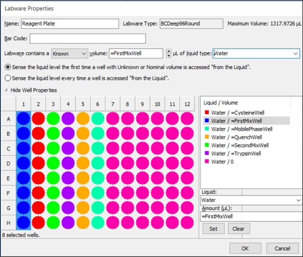
Figure 4: Properties of the reagent plate. Shown are properties needed for the Reagent Plate labware when accessed using the Guided Labware Setup. Select the corresponding column and type in the variables as indicated in the figure. Please click here to view a larger version of this figure.

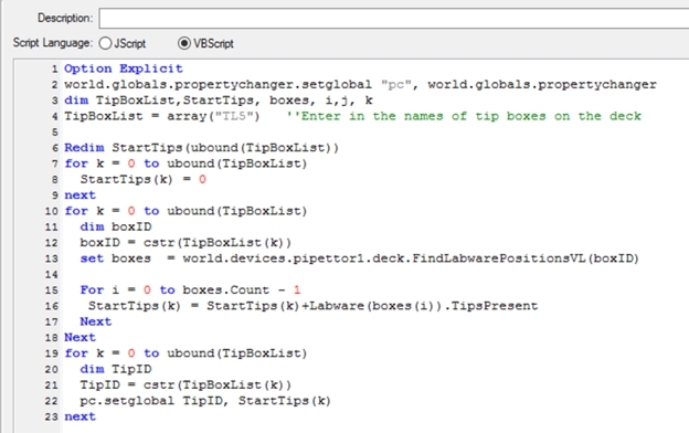
Figure 5: Tip counting script. This script helps to keep track of number of tips on the deck. Please click here to view a larger version of this figure.

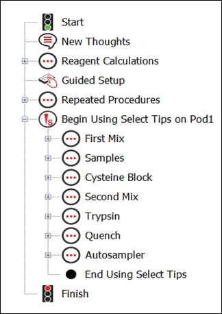
Figure 6: Overview of the method for digesting and aliquoting plasma samples. Steps for reagent calculations, labware setup, and liquid manipulations in the liquid handler’s method. Please click here to view a larger version of this figure.

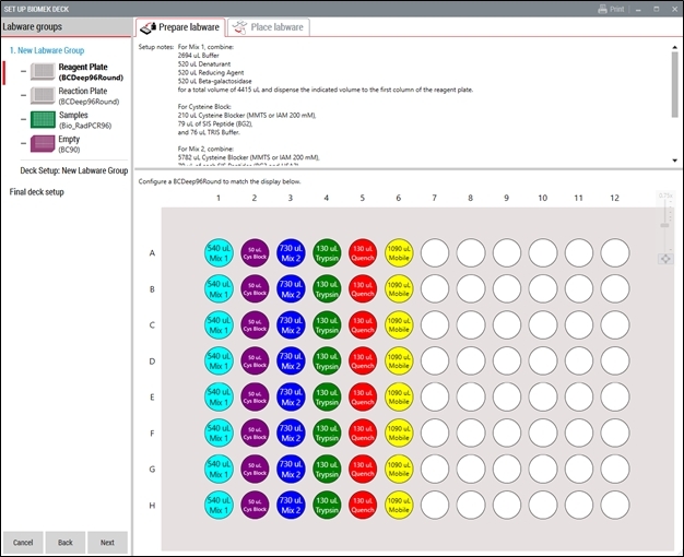
Figure 7: Layout of the reagent plate. Shown are the chemical reagents needed for plasma digestion and autosampler preparation and distributed across the reagent plate labware. This figure has been modified from a technical note¹⁰. Please click here to view a larger version of this figure.

Figure 8: Layout for the labware on the deck of the automated workstation. Shown is the deck layout for the plasma digestion method for the liquid handler. This figure has been modified from a technical note¹⁰. Please click here to view a larger version of this figure.

Figure 9: The precision of total proteomic workflow is comprised of workstation CV and targeted LC MS/MS CV.
Five peptides from β-gal and albumin were monitored, the chromatograms and peptide retention time for each peptide is shown (A), Precision was determined from 30 wells/samples processing representative experiment, CVs% for total proteomic workflow, LC MS/MS analysis and automated sample processing were calculated (B). Overall, the digested peptides showed good signals ranged from 1x10⁵ up to 1x10⁸. Please click here to view a larger version of this figure.

Figure 10: Determination of precision for liquid transferring steps. Synthetic peptides were spiked in step specific reagents, and automated liquid transferring was determined by total%CV. From 30 wells/samples experiment minus% CV LC MSMS (determined by 8 repeat LC MSMS injections. Please click here to view a larger version of this figure.

Figure 11: Multi-days reproducibility of automated proteomic sample preparation workflow with 42 protein MRM analysis. (A) Reaction plate map for each of three days is show here, 5 µL plasma was added to each of 21 wells. 3 wells received 5 ul water were used as negative/blank controls. (B) The average intensities of 190 transitions comprise of 75 peptides and 42 proteins (left) and%CV for each MRM transition was calculated from 21 wells digestion for each day (right). Please click here to view a larger version of this figure.

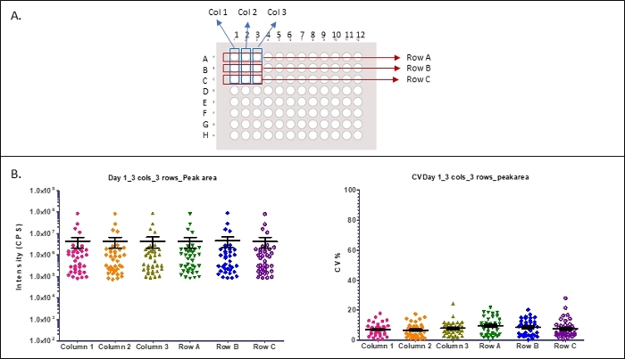
Figure 12: Reproducibility of specific locations of wells (position of columns and rows). (A) Columns and Rows location with a plate map are shown here. (B) Column and row location specific MRM signals of average intensities from specified wells (left) and cv% (right) from a single plate digestion. Please click here to view a larger version of this figure.

Figure 13: Screen shot of technique editor. For each Pipetting template, define the properties of liquid level sensing, Clot detection, Piercing, Liquid Type, General, Aspirate, Dispense, Mix and Calibration. The template and techniques used in this protocol are shown in Supplemental Table 2). Please click here to view a larger version of this figure.

Variable	Variable	Value	Description
Autosampler	Boolean	TRUE	Use autosampler
Betagal	Integer	5	Betagal volume
BG1	Integer	0.8	BG1 volume
BG2	Integer	0.8	BG2 volume
BG3	Integer	0.8	BG3 volume
CysteinBlocker	Integer	1.25	Cysteine blocker volume
CysteineBuffer	Integer	0.45	Cysteine buffer volume
Denaturant	Integer	5	Denaturant volume
DigestTransfer	Integer	10	Digest transfer volume
First Buffer	Integer	25.9	First buffer volume
First Column	Integer	1	First Column
HSA1	Integer	0.8	HSA1 volume
HSA2	Integer	0.8	HSA2 volume
lastcolumn	Integer	12	Last Column
MobilePhase	Integer	90	Mobile phase volume
Quench	Integer	10	Quench column
ReducingAgent	Integer	5	Reducing agent column
Sample	Integer	5	Sample column
SamplePlate	Boolean	TRUE	Use sample plate
SecondBuffer	Integer	58.4	Second buffer volume
Trypsin	Integer	10	Trypsin column

Table 1: Start step variables

Value	Variable
=FirstBuffer+Denaturant+ReducingAgent+Betagal+BG1+HSA1	FirstMix
=CysteineBlocker+CysteineBuffer+BG2	CysteineMix
=SecondBuffer+BG3+HSA2	SecondMix
=(FirstMix*Columns)+30	FirstMixWell
= (CysteineMix*Columns)+20	CysteineWell
=(SecondMix*Columns)+10	SecondMixWell
=(Trypsin*Columns)+10	TrypsinWell
=(Quench*Columns)+10	QuenchWell
=(FirstMixWell*8)+100	FirstMixStock
=CysteineWell*8+20	CysteineMixStock
=(SecondMixWell*8)+100	SecondMixStock

Table 2: Volume mix variables

Type	Name	Position	Depth	Properties	Use?
BCDeep96Round	Reagent Plate	P5	1(top)	#	=not SamplePlate
BCDeep96Round	Reagent Plate	P5	1(top)	#	=SamplePlate
BCDeep96Round	Reaction Plate	P11	1(top)		TRUE
Bio_RadPCR96*	Samples	P9	1(top)		=SamplePlate
Bio_RadPCR96*	Autosampler Plate	P10	1(top)		=Autosampler
BC90	Empty		1(top)		TRUE
BC90			1(top)		TRUE
BC90			1(top)		TRUE
BC230			1(top)		=Autosampler
BC90			1(top)		=Columns>1
BC90			1(top)		=Columns>3
BC90			1(top)		=Columns>5
BC90			1(top)		=Columns>7
BC90			1(top)		=Columns>9
Note: *: Corresponds to the 96 well Bio-Rad plate. #: Click properties and then enter the volume variables as indicated in Figure 6.

Table 3: Setting up the guided setup

Protein ID	Peptide sequence	Q1 Mass (Da)	Q3 Mass (Da)	Time (min)	Fragment Ion	Declustering Potential	Collision energy	Collision Cell Exit Potential
sp|P00722|BGAL_ELOCI	GDFQFNISR	542.3	262.1	19.7	+2y2	61	21	8
		542.3	636	19.7	+2y5	61	25	12
		542.3	764.2	19.7	+2y6	61	25	18
	IDPNAWVER	550.3	436.1	18.1	+2y7+2	61	23	8
		550.3	871.2	18.1	+2y7	61	25	18
		550.3	774.2	18.1	+2y6	61	33	8
	WVGYGQDSR	534.3	782.1	12.1	+2y7	51	25	6
		534.3	562.1	12.1	+2y5	51	27	6
		534.2	505.2	12.1	+2y4	90	25	8
sp|P02768|ALBU_HUMAN	DDNPNLPR	470.8	596.2	9.2	+2y5	61	27	16
		470.8	499.3	9.2	+2y4	61	27	18
		470.8	710.4	9.2	+2y6	61	27	18
	LVNEVTEFAK	575.3	694.4	18.2	+2y6	73.1	29.6	18
		575.3	937.5	18.2	+2y8	73.1	29.6	18
		575.3	823.4	18.2	+2y7	73.1	29.6	18

Table 4: MRM parameters

Supplemental Table 1: Reagent plate Please click here to download this table.

Supplemental Table 2: Protocol template Please click here to download this table.

Discussion

Sample processing for mass spectrometry requires protein denaturation, reduction and alkylation to block cysteines, and trypsin digestion to cleave proteins into peptides. Each chemical or enzymatic reaction needs to be initiated at a designated time and performed at a controlled temperature, and every step in the process involves multiple liquid transfer steps where experimental variation can be introduced. Automated sample processing provides a solution to this dilemma. Presently available liquid handling systems have the capability to transfer reagents into 96-well plates with an accuracy and precision of less than 5%, depending on the head and tip type used, and to incubate samples, with shaking if desired, under controlled temperatures ranging from 14 °C to 70 °C. We used an automated liquid handler to process plasma for SRM assays in a 96-well format.

There are many thousands of protease cleavage sites within the complex mixtures of proteins in serum, plasma, and other biological samples; and each of these proteins has unique properties affecting cleavage site accessibility and the stability of the resulting peptides. It is, therefore, impossible to design a sample processing procedure that is optimal for every protein. The best alternative is to be as consistent as possible.

To achieve consistency, we optimized each pipetting step performed by the automated liquid handler. We first considered the volume required and constraints imposed by the liquid’s type (plasma, aqueous, or organic) and corresponding properties (viscosity, cohesion, and volatility), hardware (workstation pipetting-head and plate-grabbing arms), and labware. We then varied the speed and trailing air gap for aspiration, the speed and blowout volume for dispensing, and the force and duration of mixing, while incorporating a tip touch after aspiration and/or dispensing, if needed, to eliminate liquid adhering to the outside of the tips (Figure 13, Supplemental Table 1). A unique SIL peptide, pre-screened for stability, was spiked into each reagent to make it possible to monitor the precision of each liquid handling step. After optimization, the process CVs for the majority of the transitions were less than 10%, demonstrating good reproducibility with the automated workstation (Figure 9, Figure 10, Figure 11 and Figure 12).

The automated workflow presented here provides for consistent enzymatic digestion with improved reproducibility and throughput compared to manual methods (Figure 9, Figure 10). This approach promises to improve the accuracy and reliability of biomarker discovery and validation by mass spectrometry.

Materials

List of materials used in this article

Name	Company	Catalog Number	Comments
A Pooled healthy human plasma	Bioreclamation Inc.		human plasma tested in the manuscript
Acetonitrile, HPLC Grade	Thermo Fisher Scientific	A998SK1	LC MS/MS solvent
B-Galactosidase Recombinant from E.Coli	Sigma-Aldrich	G3153-5MG	exogenous control proteins.
Biomek i7 Automated Workstation	Beckman Coulter, Inc.		The proteomic sample preparation workstation: Biomek automated workstations are not intended or validated for use in the diagnosis of disease or other conditions
Biomek i-Series Tips 230µL Non-Sterile	Beckman Coulter, Inc.	B85903	Tips, i7 consumable
Biomek i-Series Tips 90µL Non-Sterile	Beckman Coulter, Inc.	B85881	Tips, i7 consumable
FG, Kit Trypsin TPCK	Sciex	4445250	Trypsin used in digestion
Hard-Shell 96-Well PCR Plates, low profile, thin wall, skirted, green/clear	Bio-Rad	#hsp9641	Autosampler plate
Octyl B-D-Glucopyranoside	Sigma-Aldrich	O9882-5G	detergent used in digestion
Polypropylene, 96-Round Deep Well Plates Sterile	Beckman Coulter, Inc.	267007	Reagent and digestion plate
Prominence UFLCXR HPLC system	Shimadzu, Japan		High flow LC sytem
QTRAP 6500	SCIEX		Mass spectrometer
Water, HPLC Grade	Thermo Fisher Scientific	W54	LC MS/MS solvent
Xbridge BEH30 C18 2.1mm x 100mm	Waters	186003564	LC MSMS column