Worm-align and Worm_CP, Two Open-Source Pipelines for Straightening and Quantification of Fluorescence Image Data Obtained from Caenorhabditis elegans

Summary

Worm-align/Worm_CP is a simple FIJI/CellProfiler workflow that can be used to straighten and align Caenorhabditis elegans samples and to score whole-worm image-based assays without the need for prior training steps. We have applied Worm-align/Worm_CP to the quantification of heat-shock induced expression in live animals or lipid droplets in fixed samples.

Abstract

An issue often encountered when acquiring image data from fixed or anesthetized C. elegans is that worms cross and cluster with their neighbors. This problem is aggravated with increasing density of worms and creates challenges for imaging and quantification. We developed a FIJI-based workflow, Worm-align, that can be used to generate single- or multi-channel montages of user-selected, straightened and aligned worms from raw image data of C. elegans. Worm-align is a simple and user-friendly workflow that does not require prior training of either the user or the analysis algorithm. Montages generated with Worm-align can aid the visual inspection of worms, their classification and representation. In addition, the output of Worm-align can be used for subsequent quantification of fluorescence intensity in single worms, either in FIJI directly, or in other image analysis software platforms. We demonstrate this by importing the Worm-align output into Worm_CP, a pipeline that uses the open-source CellProfiler software. CellProfiler’s flexibility enables the incorporation of additional modules for high-content screening. As a practical example, we have used the pipeline on two datasets: the first dataset are images of heat shock reporter worms that express green fluorescent protein (GFP) under the control of the promoter of a heat shock inducible gene hsp-70, and the second dataset are images obtained from fixed worms, stained for fat-stores with a fluorescent dye.

Introduction

A relatively simple organism, the nematode C. elegans, is an extremely useful model system for studying human diseases. About 38% of the genes in the C. elegans genome have functional counterparts in humans^1,2. One of the unique characteristics of C. elegans is that it is optically transparent, enabling easy access to in vivo information regarding (sub) cellular expression of fluorescent reporters across tissues. This makes C. elegans a prime model organism for high-content screens using image-based platforms³. However, one issue that often complicates these studies is that when imaging dense populations of worms, they tend to cross and to cluster, making comparisons across individual worms challenging, clouding downstream image analysis and quantitation. 

Existing solutions that overcome this issue typically rely on the optimization of the culturing and imaging protocol, such as through the use of micro-fluidics setups⁴, allowing single worms to be captured in separate images^5,6. Others have applied machine-learning algorithms allowing for recognition of single worms, even in a clumped population. An excellent example of the latter is the WormToolbox, which is a modular extension of the open-source image analysis platform, CellProfiler⁷. WormToolbox offers a high-throughput and high-content solution for analysis of C. elegans, and clearly benefits from its inclusion in CellProfiler, as additional analysis modules can easily be included. Although WormToolbox comes supplied with a pre-trained model (DefaultWormModel.xml), retraining of the machine-learning algorithm is usually required for each new application. Online tutorials on how to do this are available on Github (https://cp-website.github.io/Worm-Toolbox/). Despite this, installing and using WormToolbox requires a significant time-investment for novice users. 

Here, we describe a simple and cost- and time-effective protocol to culture, and image populations of C. elegans. To allow the assessment of individual worms in the acquired images we have developed a simple open-source FIJI-based workflow, named Worm-align. Worm-align can be used to generate single- or multi-channel montages of straightened and aligned worms. Firstly, the user must manually select individual worms for analysis by drawing a line from the head to the tail. Worm-align will use this selection to crop selected worms from the overview image, and generate a montage in which selected worms are straightened and aligned to facilitate visual comparison and presentation. 

In addition, the output of Worm-align can be used for subsequent quantification of fluorescence intensity in single worms, either in FIJI directly, or in other image analysis software platforms. We demonstrate this by importing the Worm-align output into Worm_CP, a pipeline that uses the open-source CellProfiler software. CellProfiler’s flexibility enables the incorporation of additional modules for high-content screening. We have used the Worm_CP pipeline to quantify the heat shock response, a well conserved protective mechanism that refolds proteins that are misfolded due to stressors such as high temperature⁸. Specifically, we applied the pipeline to worms carrying an integrated multi-copy transgene, where the promoter of a heat shock inducible gene, hsp-70(C12C8.1), drives green fluorescent protein (GFP)⁹. We have also used the Worm_CP pipeline on fixed animals that have been labelled with a fluorescent dye that visualizes lipid droplets (LDs), the main fat storage organelle in C. elegans¹⁰. While this workflow does not have the throughput offered by WormToolBox, it is a user-friendly and simple alternative for visual presentation and analysis of image-based C. elegans experiments.

Protocol

1. Fixation of worms for fat-content imaging using a fluorescent dye for lipid droplets (BODIPY)¹⁰

1. Prepare a synchronized population of C. elegans by bleaching according to standard procedures². Plate about 1,000 L1-stage worms onto a 9 cm nematode growth media (NGM) plate per condition.
   NOTE: More worms are prepared than actually quantified at the end, due to loss of worms when handling.
2. To image animals at young adult stage (around 50 h post L1 plating at 20 °C), wash each 9 cm plate with 15 mL of M9 in a conical tube, centrifuge at 252 x g for 1 min, and remove the supernatant. 
3. Repeat the wash and leave 1 mL of M9 over the pellet of worms.
4. Transfer 1 mL of M9 containing the worms in a 2 mL low protein binding microcentrifuge tube, using low retention tips.
5. Spin down at 252 x g in a microcentrifuge for 1 min and remove the supernatant, being careful not to touch the worm pellet at the bottom of the tube.
6. For monitoring fat content using 4,4-difluoro-1,3,5,7,8-Pentamethyl-4-bora-3a,4a-diaza-s-indacene (BODIPY) staining¹⁰ (Table of Materials), fix worms either by adding 0.5 mL of 60% isopropanol to the worm pellet for 3 min¹¹, or by adding 2 mL of ice-cold methanol for 10 min. For both procedures, invert the tube every 30 s. 
   CAUTION: If methanol is the chosen fixation reagent, this step must be undertaken in a fume hood due to its toxicity.
7. Remove as much fixative as possible without touching the worm pellet and add 1 mL of M9. Let the worms settle at the bottom of the tube for 3−5 min.
8. Wash again with 1 mL of M9, let the worms settle and remove the supernatant, leaving about 50 µL in the tube. Secure the tube using a clamp. 
9. Freeze-crack the worms by plunging the securely closed tube in liquid nitrogen and then into a warm water bath at ~40 °C.
10. Repeat step 1.9 one more time.
11. Add 0.5 mL of BODIPY diluted in M9 at a final concentration of 1 µg/µL and place on a rotator at room temperature for 1 h.
12. After 1 h, let the worms settle at the bottom of the tube for 3−5 min. 
13. Remove supernatant and add 1 mL of M9.
14. Let the worms settle at the bottom and remove supernatant. 
    NOTE: Alternatively, it is possible to spin down at 252 x g for 1 min, as this does not seem to affect the morphology.
15. Add 0.5 mL of M9. 
    NOTE: If the fixative is 60% isopropanol, the worms can only be utilized within 48 h. If the fixative is methanol, the worms should be utilized within 24h.

2. Preparing agarose pads to mount the worms

NOTE: The critical step while preparing an agarose pad is to obtain a pad of regular thickness. Otherwise, worms across the pad will be in different focal planes, making it tricky to get a focused image of a wider field of view. 

1. Prepare 2% agarose pads by adding 0.2 g of agarose to 10 mL of sterilized H₂O in a beaker or a conical flask. Heat in the microwave for 30 s until the agarose starts boiling. 
   NOTE: Do not overheat and stop as soon as bubbles appear; otherwise it increases the viscosity of the agarose making it harder to achieve the desired pad thickness.
2. Once the agarose is melted, dispense a drop of melted agarose in the center of a microscope glass slide using a 1000 µL pipette tip with its very end cut. Immediately, but delicately, hold another glass slide very close to the agarose drop and release it onto the agarose to form a pad of regular thickness for best microscopy results.
   NOTE: Releasing the top slide from a height will not only form bubbles but will result in an uneven pad. Alternatively, it is also possible to use two glass slides flanking the slide with the pad, with a thin layer of tape on each slide. 
3. After a minimum of 2−3 min, gently remove the top slide. Using the side of the top slide, trim the pad to make it square shaped. Mount the worms within 5 min, to prevent the pad from drying before use.

3. Mounting fixed worms for imaging

1. Create a mouth micropipette by extending a thin glass capillary in the flame of a Bunsen burner (Figure 1A). After extension in the flame, break the capillary into two pieces (Figure 1B). Choose the most adequate, usually the longest, and test whether the end of the capillary is open by trying to aspirate water. 
   NOTE: If the liquid does not come into the capillary, it is too thin or blocked. Gently cut the end of the capillary with a pair of scissors, avoiding cutting too much as worms will be aspirated if the hole is too big. 
2. Plug the glass capillary from step 3.1 into the capillary adaptor (Figure 1C), linked to the 6 mm silicone tube and plug the other end of the 6 mm silicone tube into a 0.2 µm filter, attached to a 3 mm silicone tube on its other end (Figure 1C). Plug a 1 mL filter tip (Figure 1C) into the free end of the 3 mm silicone tube to aspirate liquid.
   NOTE: The 0.2 µm filter is added between the mouth of the experimenter and the capillary, to ensure maximum safety of the experimenter. A similar solution is used for mouth micropipettes used to handle mouse embryos¹². Change the filter (usually every few months) if the mouth micropipette is not aspirating liquid anymore.
3. Using the mouth micropipette under a dissection microscope, remove as much liquid as possible around the worm pellet of fixed worms (Figure 2).
   NOTE: Pipetting supernatant out using a manual micropipette can be used as an alternative to the mouth pipettes in steps 3.1 to 3.3 to remove as much supernatant as possible. Add 6 µL of mounting medium. We find, however, that this method does not work as efficiently because excessive liquid in the pads creates a sparse worm density, which makes imaging more time-consuming. Resume step 3.6. Look at the bottom of the tube and make sure that the pipette does not aspirate the worms. 
4. Quickly add 10 µL of mounting medium (Table of Materials) to the bottom of the tube.
5. Rinse a 10 µL tip in PBS with traces of detergent (0.01% Triton), to prevent worms from sticking to the sides of the plastic pipette tip. Cut the very end of the tip with a pair of scissors.
6. Transfer 8 µL of mounting medium containing the worms onto the agarose pad prepared in step 2.3. Under the microscope, gently shake the slide, to avoid overlap of the worms.
7. Cover the drop of mounting medium on the agarose pad with an 18 mm x 18 mm coverslip (Figure 3).
   NOTE: Smaller coverslips are preferred as they exert less pressure onto the worms. Hold the coverslip with a pair of tweezers and apply one edge of the coverslip against the agarose pad, before gently depositing the coverslip with the tweezers.

4. Mounting live worms for imaging

NOTE: To image live worms, they have to be immobilized on the pad. One way to achieve this is to paralyze them with the nicotinic receptor agonist: levamisole (Table of Materials).

1. Pipette 3−4 µL of 3 mM levamisole dissolved in M9 onto the agarose pad created in step 2.3.
   NOTE: There should be enough liquid volume that the worms are not on top of each other but not too much liquid that the worms are too sparse on the pad. Experienced worm pickers can use 3 µL of levamisole. Less experienced pickers might need to add a larger volume of levamisole, so that the levamisole does not totally evaporate.
2. Pick 30−50 worms per condition into the drop of levamisole.
3. Cover the drop of levamisole on the agarose pad with an 18 mm x 18 mm coverslip. Image worms within 1 h, as the paralyzing agent will eventually lead to death of the worms.

5. Imaging slides with an epifluorescence microscope 

1. With an agarose pad of uniform thickness, image all worms on the slide at once using a 6 x 6 or 7 x 7 large image for instance with the 20x objective of a fluorescent microscope. If the thickness of the pad is not even, acquire several smaller 3 x 3 or 4 x 4 images of the same slide. 
2. Use the same settings for fluorescence intensity and exposure time for all conditions. Adjust each setting to match the slide that has the brightest intensity, ensuring that there is no pixel saturation. For specific instructions on image acquisition, follow the microscope manufacturer’s instructions. 

6. Creating montage images of aligned single worms using the Worm-align FIJI pipeline

1. Install the open-source image analysis software package FIJI¹³/ImageJ¹⁴ from https://imagej.net/Fiji. If a prior installation of FIJI is available, ensure it is updated to version 1.52a or later, as some of the functions used in the macro (e.g., Table functions) require this. Download the Worm-align macro from Github: https://github.com/hannekeo/Worm-align.
2. Open FIJI and run the Worm-align macro. Execute Worm-align by clicking Plugins | Macros | Run in the FIJI main menu bar (Figure S1). Now locate the Worm-align.ijm script on the computer.
3. The macro initializes by asking for the location of the images. The pipeline will work on both single-channel and multi-channel fluorescence images (Figure S2). Select an input folder and the macro will automatically generate an output folder where all results will be saved (Figure S3).
   NOTE: It is important that the selected folder contains only image files as the presence of other file formats will cause the macro to crash. Ideally, only group together images that were captured with the same microscope settings. Worm-align will accept many different file formats, including nd2, czi, tif, rgb, jpg and png. The name of the output folder will be the same as the input folder, with ‘_output’ added as a postfix, i.e. if the input folder is ‘images’, the output will be found in ‘images_output’. The output folder will contain four subfolders, in which the data will be saved.
4. Allow the macro to proceed to open the first image in the input folder and use it as a representative image to extract a setting to generate the montage.
   NOTE: Worm-align will automatically select the first image in the input folder to generate the settings that will be applied to all other images in the folder. If another image is deemed to be more representative of the dataset, ensure this image is selected by saving a copy of the image in the input folder, changing the name so that is now listed at the top of the list (e.g., ‘0_RepresentativeImage’).
5. With the Straight-line drawing tool, draw a line across the width of a worm (Figure S4) and use the length of this line to determine the height of the cropped regions for single worms. For each channel, specify the name, lookup table (LUT), intensity settings (B&C) and whether it should be included in the montage (Figure S4).
   NOTE: These parameters are recorded and saved in a settings file, Settings.csv, located in the CellProfiler subfolder of the output folder.
6. Once all settings have been captured, the user is shown what the images will look like after application of the settings applied (Figure S5). Tick the top box if the settings are sufficient. Select options for montage generation (remove ticks, if not required): 1. Generate a montage of selected worms for each single image, or 2. Generate a combined montage in which all worms selected on all images in the input folder will be combined into a single montage. Click OK to execute the rest of the macro. 
   NOTE: If the top box is not ticked before clicking ‘OK’ the macro will rerun the setup, so image settings can be optimised.
7. The Worm-align pipeline now proceeds to open all images in the input folder. For each image, draw lines on the longitudinal axis of all worms to be included in the montage and/or quantify (Figure 4 and Figure S6) using the ‘segmented line’ tool (on the FIJI main menu bar). To ensure proper alignment of worm, draw lines consistently from head to tail end (or vice versa), and along the full length of the worm (see examples of “good” and “bad” line drawing in Figure 4B).
8. Add each line to the ROI manager, by clicking Ctrl+T. Worm-align uses the lines added to the ROI manager, in combination with the worm width parameter (set in step 6.4) to generate cropped images of single selected worms. The collection of line ROIs is saved in the ‘data’ subfolder. This folder also contains a copy of the original image showing the lines, as well as the number of the worm. Lines are color-coded with the Glasbey_on_dark lookup table. The images of straightened worms are saved in the single_worms subfolder of the output folder. In addition, if selected in step 6.6 of this protocol, Worm-align produces montages of all worms selected per overview image and/or for all overview images in the input folder (see Figure 4C and Figure S7). These montages can be found in the ‘aligned’ subfolder of the output folder. 

7. Analyzing single-worm fluorescence intensity using the output from Worm-align in an automated CellProfiler pipeline

1. For downstream data processing and analysis of the Worm-align output, download and install the open-source image analysis software package ‘CellProfiler^15,16 from https://cellprofiler.org/. Download the Worm_CP.cpproj pipeline from GitHub: https://github.com/hannekeo/Worm-align
   NOTE: The example pipeline described here was constructed using CellProfiler2.2.0 and might not run in later versions of CellProfiler.
2. Before starting the Worms_CP.cpproj pipeline, ensure that all expected output images are present in the CellProfiler subfolder of the Worm-align output folder: a processed copy of the original image (named: Original_), a binary image mask of the worm population (named: Mask_), a line mask of the lines drawn on selected worms (named: Lines_), and one image representing each of the channels present in the original image (named by channel number).
3. To quantify the fluorescence intensity in single worms, click on the Images input module and simply drag the CellProfiler output folder into the window that says Drop files and folders here. If a list of images is present from previous analysis, first remove these by right clicking in the window and selecting Clear File List. To exclude the ‘Settings.csv’ file from the images list, select either ‘Images only’ or ‘Custom’ with ‘Extension is tif, tiff, ome.tif, or ome.tiff’ for the filter settings (Figure S8).
4. Click on the Metadata input module. In the second extraction method, click on the yellow folder, and locate the CellProfiler subfolder in the WormAlign output folder (Figure S9). Select the Settings.csv file and link the settings in the file to the CellProfiler output by matching the metadata in the CSV files to those in the images (Channel metadata). 
5. Click on the NamesAndTypes input module and insert a new image for each channel of the original image to be quantified.
   NOTE: Already present in the example pipeline are the worm mask, two color images, the line mask and the original image, and three grey scale images (the green and the red channel). The list in this module needs to be adjusted if the original images have more or fewer channels than the example images.
6. Check that the name of the images in every column label/mask/worms is correct.
   NOTE: The names of the images on one line should all correspond to the same initial image to analyze. If a mistake is made during the image analysis process, some of the output images will be missing and the names under the three columns label/mask/worms will not correspond to the same initial image anymore for each line. If this is the case, find where the mistake is.
7. Press View output setting to select the folder to save the output from Cellprofiler. 
8. Click Start Test Mode. Once in Test Mode, double-check the settings of the pipeline by applying them to the first image in the dataset, by clicking Run (which will run through all active modules in the pipeline), or Step (which will run through the pipeline one module at a time).
   NOTE: While in the Test Mode, the extracted measurements will not be exported, even if an ExportToSpreadsheet module is present (and active) in the pipeline.
9. Once the pipeline performs the way it should, click Exit Test Mode and then press Analyze Images. As currently configured, the Worms_CP will (1) use the Mask_ image to segment a rough worm mask and the Lines_ image (Figure S10A) to single out the selected worms and produce single worm masks (Figure S10C), (2) measure the fluorescence intensity of all channels present in the input images in those worms identified and masked. The pipeline can also measure background intensity (Figure S10B) and correct all images accordingly (indicated by the word threshold in the name of the parameter measured. e.g.: Intensity_MeanIntensity_green_threshold), (3) measure the size of the selected worms, and (4) export all measured parameters (Figure S10D).
10. Open the Worm_CP output consisting of two csv files, worms.csv and lines.csv that are saved in the selected output folder (see Figure S11). These files can be opened in Excel or R (Studio) for post-processing and reporting. If additional output is required, e.g. per image data, this can be selected in the ExportToSpreadsheet module in the pipeline. 

Results

Culturing and imaging C. elegans according to the method described in this protocol produces large overview images of worm populations. To facilitate visual inspection and classification of worms from these images we have developed Worm-align. Worm-align is a simple and user-friendly FIJI script that can be used to create montages of straightened and aligned worms. Worms are selected from overview images by drawing a line along the longitudinal axis of the worms. Each selected worm is assigned a number, cropped and straightened, and added to a montage. Montages can be generated per image or combining all images from the original input folder. 

As expected, the output of the pipeline largely depends on the quality of the lines drawn on top of the images. To illustrate this point, Figure 4 shows several line examples, and their output from Worm-align. A complete line from the head to the tip of the tail produces a properly aligned worm (labelled “good”). Figure 4 also shows how tracing inaccuracies during the execution of Worm-align affect the output of the alignment. From the annotated montage included in Figure 4C, care should be taken to avoid the following errors, as they hinder the proper alignment of worms:

• Inconsistent tracing of the worm from head to tail (labelled “tail to head”). This results in worms being orientated in different directions (i.e., tail-to-head versus head-to-tail) in the alignment.
• Incomplete tracing (labeled “incomplete”). This results in only the part of the worm that was traced to be cropped for the montage.
• Including multiple worms in a single trace (labeled “worm with two heads”). This results in worms plus (significant sections of) their neighbors being inserted in the same panel of the montage.
• Adding random lines to the image (labeled “random”). This results in the insertion of random panels in the montage.

For creation of the montage it is not an issue if two individual lines intersect (labeled “intersecting”) or are joined at either end of the worm (labeled “joined”), as long as each line traces the entire length of an individual worm: The Worm-align script individually and sequentially selects each line ROIs, crops and straightens it, so that each panel in the final montage will represent a single line trace. In case of the intersecting worms however, although full length straightened worms appear for worm “intersecting1” and worm “intersecting2” in the montage (see Figure 5A-B), it is clearly noticeable that these worms cross each other in the original overview image. Therefore, it can be concluded that visual identification of intersecting lines is possible from the overlay image found in the ‘data’ subfolder (Figure 5A), as well as from the panels of individual worms in the montage (Figure 5B). In addition, any overlap of worms/lines can be identified from the quality control (QC) table generated for each processed image by Worm-align, and saved in the data subfolder. This table records three parameters for each of the line ROIs drawn in the image (see Figure 5C): Of these, Length indicates the length of the line ROI, which is a good indicator of the size of the worm; and the Worm number indicates the order in which the lines were drawn on the overview image. Finally, the last column indicates whether there is overlap between the worm/line in question and any of the other worms/lines selected in the image. In case of overlap the number in this column will be different from the one listed in the Worm number column. In combination with the overlay image, the QC table should aid the researcher to make learned decisions on which worms should be excluded from the montage and/or quantification.

The output of Worm-align can be used for subsequent quantification of fluorescence intensity in single worms. In FIJI, the line ROIs can be used to measure fluorescence intensity in the original image data, for example by executing the simple FIJI script ‘ Worm-quant.ijm’, which can also be found in the Worm-align repository on Github. Alternatively, the Worm-align output can be imported into third party image analysis software. We demonstrate this by importing the Worm-align output of two datasets into Worm_CP, a pipeline we generated in CellProfiler. Worm_CP uses the files in the ‘CellProfiler’ subfolder of the Worm-align output folder to fine-tune segmentation masks of those individual worms selected during execution of the Worm-align macro. Specifically, it uses the line mask (named: Lines_) to isolate selected worms from the worm population seen in the binary mask (named: Mask_). It should be noted that lines that intersect on the overview image (Figure 5A), although not a problem for the generation of montages, are problematic for the Worm_CP pipeline. Why this is the case, is illustrated in Figure 5 D-E. Worm_CP uses the line mask (Figure 5D), and not individual ROIs to aid identification of individual worms. The intersecting line drawn second during the execution of Worm-align is superimposed on the first line and therefore the intensity along this line will be that of ROI2 including in the bit where line 1 and 2 overlap. As a result, CellProfiler will segment line2 as one object, but line1 as two objects that are separated where it intersects with line2. This means that CellProfiler will produce two (half) worm masks for worm ‘intersecting1’ (Figure 5E). The easiest way to exclude these events from the final analysis (if required), is to identify the worm number of intersecting worms from the QC table (data subfolder), and to remove measurements for these worms from the CellProfiler output files. Please note that worms will not necessarily be allocated the same number in FIJI and CellProfiler: To identify the FIJI worm number in the CellProfiler output look at the Intensity_Max_Intensity values in the ‘Lines.csv’ output file. Any Intensity_Max_Intensity value that appears in the ‘Lines.csv’ table more than once per image is an indication of that line ROI resulting in a fractured worm mask.

Once individual worm masks are segmented, Worm_CP can measure the fluorescence intensity in the selected worms for all recorded channels. All measurements are taken from the original (raw) image data, although it should be noted that CellProfiler automatically rescales the pixel intensity on a scale of 0-1. This is achieved by dividing the raw pixel intensity value by the maximum possible pixel intensity for the image. In case of 8-bit images this value is 255, and in case of 16-bit images it is 65535. CellProfiler intensity values therefore need to be multiplied by the maximum possible intensity value to regain values equivalent to the raw image data. The Worm_CP output consists of two csv files, ‘worms.csv’ and ‘Lines.csv’ that are saved in the selected output folder. While inspecting these files, it is clear that CellProfiler records a large number of parameters related to fluorescence intensity. Of these, the Intensity_IntegratedIntensity corresponds to the total fluorescence per worm (i.e., the sum of the fluorescence intensity within all pixels that construe the mask of an individual worm). The parameter Intensity_MeanIntensity refers to the average fluorescence intensity within an individual worm (i.e., the average fluorescence intensity per pixel for all the pixels contained within an individual worm). Due to the occasional occurrence of (small) errors in segmenting the worm masks it is recommended that MeanIntensity measurements are used when comparing fluorescence measurements of individual worms between two conditions. If wanting to substract the background fluorescence from quantified measurments, use the measurments named MeanIntensity_Threshold.

We have used the Worm_CP pipeline to quantify fluorescence intensity from fixed animals that have been labelled with a fluorescent dye that incorporates into lipid droplets (LDs) (Figure 6). In order to validate fluorescence quantification from the Worm-align/Worm_CP pipeline, we quantified fluorescence intensity in the same set of worms from the BODIPY dataset by either the Worm-align/Worm_CP pipeline or manual quantification in FIJI/ImageJ. Manual quantification was performed in FIJI/ImageJ by circling each worm as well as a dark background zone in every image. The fluorescence intensity was measured in the ROI manager and the value measured for the image background was subtracted from the worm fluorescence measurement of each worm, as described¹⁷. We compared wild type (WT) N2 worms to dbl-1(nk3) mutants, which exhibit decreased lipid droplet content¹⁸. As expected, the green fluorescence intensity is significantly decreased between WT and dbl-1(nk3) worms with both methods (Figure 6A,B). Examples of aligned worms can be observed in Figure 6C,D. The lipid droplet content is decreased by 17% (p-value<0.0001, unpaired t-test) between WT and dbl-1(nk3) using manual quantification, and by 14% (p-value=0.0051 unpaired t-test) using the Worm_CP pipeline. The decrease in lipid droplet content observed here in dbl-1(nk3) with both quantification methods is in accordance with the literature¹⁸. This shows that quantification of acquired fluorescence images with the Worm_CP CellProfiler pipeline is comparable to manual quantification. 

We have also used Worm_CP to quantify the heat shock response in live worms expressing GFP under control of the heat shock inducible gene hsp-70(C12C8.1)⁹. Figure 7 shows representative images of live C. elegans carrying the heat-responsive hsp-70(C12C8.1)p::GFP reporter. In the absence of heat stress, the worms do not induce GFP expression (Figure 7A,B). However, when worms are exposed to a short heat-shock of 30 min at 34 °C, they induce GFP expression (Figure 7C,D). GFP expression levels with and without heat-shock are quantified in Figure 7E.

As it stands, Worm_CP is a very basic pipeline. However, this approach does enable a more accurate segmentation of individual worm masks, which allows for a more accurate quantification of the fluorescence intensity in those worms selected from the image. For this reason, we prefer this approach over a rough quantification in FIJI, using just the line masks. In addition, CellProfiler offers the advantage that additional analysis modules can easily be included in the pipeline. For example, for the dataset that looks at lipid droplet content, insertion of additional modules into the Worm_CP pipeline could investigate lipid droplet numbers and fluorescence intensity of individual droplets in those worms selected in the overview images.

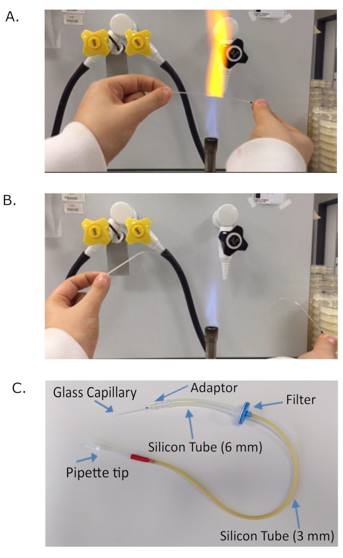
Figure 1: Generating a mouth micropipette. A glass capillary is extended in the flame of a Bunsen burner (A), until it provides thin elongated extremities (B). The extended glass capillary is then plugged into the adaptor piece of the mouth micropipette. (C) Schematic of a mouth micropipette. The mouth micropipette was assembled with a glass capillary plugged into an adaptor. A 6 mm silicone tube connects the adaptor to a 0.2 µm syringe filter, used for safety. The other end of the filter is attached to a 3 mm silicone tube ending with a 1mL filter tip. The experimenter can aspirate via the filter tip. Please click here to view a larger version of this figure.

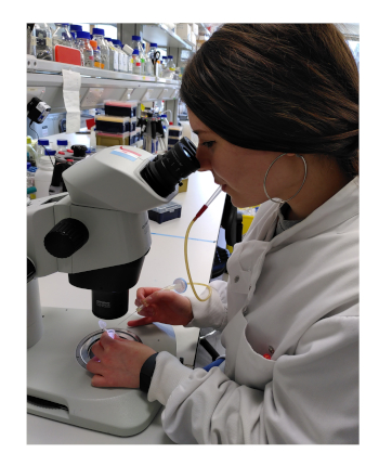
Figure 2: Aspiration of the liquid surrounding the worm pellet, using the mouth micropipette. Please click here to view a larger version of this figure.

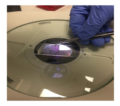
Figure 3: Adding the coverslip onto the worms laying on the agarose pad Please click here to view a larger version of this figure.

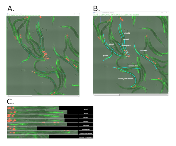
Figure 4: Examples of worm straightening using Worm-align on fluorescence images acquired from live animals carrying the transcriptional reporter fat-7p::GFP in the intestine and a red co-injection marker in the pharynx (myo-2p::tdtomato). (A) Screenshot of a composite image acquired on the fluorescent microscope of live worms at day 3 of adulthood. The image was opened with Worm_align and lines were drawn along the longitudinal axis of the worms using Worm-align. (B) Screenshot of the same image as in (A), with examples commented of good and bad drawing of the lines along the axis of the worms, using Worm-align. (C) Examples of lines drawn on top of worms that can rise to incorrectly aligned worms. Worm-align output of the worms selected in B. Images were taken with a 20x objective on an inverted widefield microscope (see Materials table) with green fluorescence intensity=1, exposure=60 ms and red fluorescence intensity = 8, exposure=60 ms. Please click here to view a larger version of this figure.

Figure 5: Examples of worm straightening using Worm-align on intersecting worms. (A) Screenshot of a composite image acquired on the fluorescent microscope of live worms at day 3 of adulthood animals carrying the transcriptional reporter fat-7p::GFP in the intestine and a red co-injection marker in the pharynx (myo-2p::tdtomato). Intersecting worms are labelled “intersecting1” and “intersecting2”, while non overlapping worms are labelled “good3” and “good4”. (B) Montage created by Worm-align representing straightened worms selected in (A). It is noticeable in the montage that the worms 1 and 2 were intersecting on the original image (worms labelled as “intersecting1” and “intersecting2”). (C) Screenshot of the QC table from Worm-align which allows to spot cases where worms intersect. Length: length of the ROI line; worm number: order in which the lines were drawn; last column indicates whether there is an overlap between the worm/line of interest and any other worm. In this example, the worm in the first raw (worm number1) overlaps with worm number 2, as indicated by the number “2” in the last column. (D) Screenshot of the lines drawn with Worm-align on the four worms selected in A. (E) Screenshot of the masks generated by Worm-align on the four worms selected in A, showing how the masks for the two intersecting worms are rendered. In this case, two masks instead of one are now corresponding to the worm “intersecting1”. Images were taken with a 20x objective on an inverted widefield microscope (see Materials table) with green fluorescence intensity=1, exposure=60ms and red fluorescence intensity = 8, exposure = 60 ms. Please click here to view a larger version of this figure.

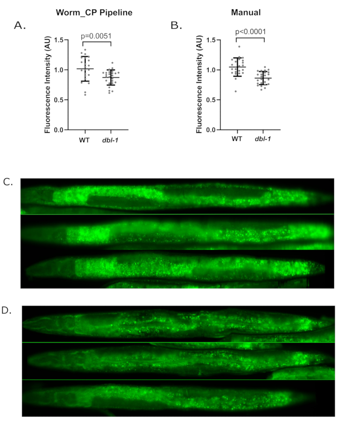
Figure 6: The Worm_CP pipeline quantifies fluorescence as accurately as would manual quantification. Comparison of fluorescence quantification of young adult worms fixed and stained for lipid droplet content with the green fluorescent dye BODIPY, using either Worm_CP pipeline (A) or manual quantification (B). The lipid droplet content of WT and dbl-1 (nk3) was monitored by fixing and staining animals with BODIPY, that intercalates into fatty acids of lipid droplets (see protocol A). Young adult animals were fixed with 60% isopropanol and stained with BODIPY for 1h. The same set of animals were quantified either using the Worm_CP pipeline (see step 7) or by manual quantification according to standard procedures¹⁷. (A) Quantification of fluorescence using Worm_CP pipeline. WT: n=22 animals, average fluorescence= 1.016 (A.U) ± 0.206 SD; dbl-1(nk3): n=25 animals, average fluorescence= 0.8714 (A.U) ± 0.126 SD. Unpaired t-test. (B) Manual quantification of fluorescence. WT: n=22 animals, average fluorescence = 1.048 ± 0.153 SD; dbl-1(nk3): n=25 animals, average fluorescence = 0.8632 ± 0.109 SD. Unpaired t-test. (C, D) Representative example or Worm-Align output for WT (C) and dbl-1(nk3) (D) animals straightened with the Worm-align pipeline. Images were taken with a 20x objective on an inverted widefield microscope (see Materials table) with green fluorescence intensity=2, exposure=60ms. Please click here to view a larger version of this figure.

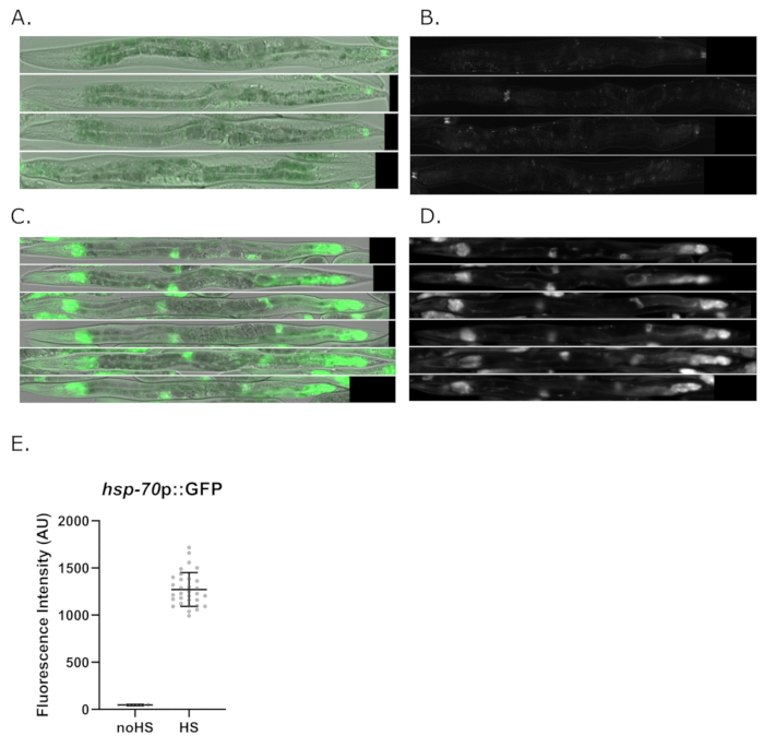
Figure 7: Example of fluorescence quantification and alignment of live worms from fluorescence images of live worms carrying the transcriptional reporter hsp-70(C12C8.1)p::GFP following heat-shock. (A) Upon a short heat-shock (30 min at 34 °C), young adult worms were recovered at their cultivation temperature (25 °C) and mounted then imaged 3.5h post heat shock. About 30 worms were quantified following heat shock using the Worm-align pipeline. (A-B) Examples of aligned worms that have not been exposed to heat shock. (C-D) Examples of heat-shocked worms carrying hsp-70(C12C8.1)p::GFP using Worm-align. (E) shows the GFP Average intensity (Worm_CP parameter: MeanIntensity_Threshold) of WT young adult worms grown, without heat shock or upon exposure to heat shock (34 °C for 30 min). Images were taken with a 20x objective on an inverted widefield microscope (see Materials table) with green fluorescence intensity=1, exposure=60ms; no HS: n=12, HS: n=32. Please click here to view a larger version of this figure.

Supplemental Figure 1: Location in FIJI where the Worm-align macro can be found, once installed. Please click here to download this file.

Supplemental Figure 2: Selection of the folder containing all images taken with the same settings. Please click here to download this file.

Supplemental Figure 3: Generation of 4 subfolders in the output folder in FIJI. Please click here to download this file.

Supplemental Figure 4: Drawing of a line across the width of the worm and channel settings for the montage. Please click here to download this file.

Supplemental Figure 5: Preview of the image with the applied settings. Please click here to download this file.

Supplemental Figure 6: Drawing of a line along the longitudinal axis of the worms of interest for inclusion in the montage and/or quantification. Please click here to download this file.

Supplemental Figure 7: Montage of the selected worms in the output folder, under “aligned” folder. Please click here to download this file.

Supplemental Figure 8: Clearing previous images from previous analysis in Cell Profiler. Please click here to download this file.

Supplemental Figure 9: Importing metadata into CellProfiler from the Worm-align output folder by selecting the Settings.csv subfolder. Please click here to download this file.

Supplemental Figure 10: The CellProfiler pipeline Worm_CP.cpproj uses the Lines_ images to single the selected worms (A), and produces single worm masks of the worms of interest (C). The pipeline also measures background intensity (B). Outlook of all the parameters measured by the pipeline Worm_CP.ccproj which are exported in a csv file (D). Please click here to download this file.

Supplemental Figure 11: Selection of output files in the “ExportToSpreadsheet in the Worm_CP.cpproj pipeline. Please click here to download this file.

Discussion

Worm-align is a FIJI-based image processing pipeline that readily generates montages of user-selected worms, in which worms are straightened and aligned to aid visual comparison, classification and representation. Although this feature is also offered by some existing tools, notably the WormToolbox module in CellProfiler⁷, Worm-align requires comparatively little prior image analysis experience: Users need only to trace those worms they would like to select for the montage (and analysis). Although tracing the worms on the raw image data is an easy process -particularly when a touch-screen computer or tablet is available-, it is paramount, that lines are correctly drawn along the longitudinal axis of the worms. Incomplete lines, that follow only part of the worm, will result in partial worms in the montage (i.e., worms missing heads of tail ends) and partial segmentation masks during CellProfiler analysis. Also, if lines from two individual worms cross, the worms will not be correctly processed in the worm alignment montage as well as for fluorescence quantification. For quality control an overlay image of the line selections on the original image is saved in the data folder, along with a QC table. From these, problematic lines that will lead to incorrectly segmented worms can readily be identified and excluded from montage and/or subsequent analysis.

Although the direct input from the experimenter in the selection of worms perhaps seems a little time-consuming, it presents a clear advantage of the workflow over others in experiments where worms from different developmental stages are present in the same image: Worms can be selected during the “tracing step”, by outlining only those worms that are in the right developmental stage. Alternatively, worms can be filtered using the output from Worm_CP based on either the length of the tracing line, or the area of the segmentation mask, both reliable indicators of the length/size of the worms. Arguably, machine-learning algorithms may struggle to recognize worms from different developmental stages, as their size and appearance in the DIC images is so different.

The output of Worm-align can be used for subsequent quantification of fluorescence intensity in single worms, either in FIJI directly, or in other image analysis software platforms. We demonstrated this by importing the Worm-align output into a simple CellProfiler pipeline (Worm_CP), which allows the quantification of multi-channel fluorescence intensity in those individual worms that were selected while running the Worm-align pipeline. We chose this approach because of the flexibility of the CellProfiler software: It is straightforward to incorporate additional modules into the pipeline to analyse additional features in individual worms (e.g. measuring the size of lipid droplets, or stress granules, nuclei, mitochondria). In addition, the single worm masks could potentially be used to train a new model for WormToolbox⁷.

The main advantages of this method are that it is fast and requires a simple worm mounting set-up. This method is faster as it does not require spending time learning software operation nor running training sets through a machine algorithm⁷. Furthermore, this method works with either live or fixed worms simply mounted on regular agarose pads. There is no need to use complex microfluidic chambers, as developed in other methods^5,6.

Materials

List of materials used in this article

Name	Company	Catalog Number	Comments
Agarose	MeLford Biolaboratories Ltd	MB1200
Aspirator tube	Sigma-Aldrich	A5177	to create mouth micro-pipette (see protocol step)
Beaker
BODIPY 493/593	Invitrogen	D3922	stock solution prepared in DMSO at 1mg/mL
Centrifuge	MSE MISTRAL 1000
Conical flask
Cover Slip	VWR	631-0120
Filter 0.2 µm for Syringe	Sartrius	16534-K	Filter, to create mouth micro-pipette (see protocol step)
Isopropanol
Levamisole hydrochloride	Sigma-Aldrich	BP212	3mM solution prepared by dissolving levamisole in M9
Liquid Nitrogen			Liquid Nitrogen facility
Low Retention Tip 1000µL	Starlab	S1182-1830
Methanol	VWR chemicals	20847.307
Microscope Slides, MENZEL GLASSER	Thermo Scientific	BS7011/2
Microscope	Nikon		Eclipse Ti
Microwave Oven	Delongi
M9			prepared in the lab according to15
9cm NGM Plates			prepared in the lab according to15
PBS			prepared in the lab
Protein LoBind Tube 2ml	Eppendorf	22431102
Triton	SIGMA	T9284-500ML
Ring Caps	SIGMA-ALDRICH	Z611247-250EA	glass micro-capillary tubes to create mouth micro-pipette (see protocol step)
Rotator	Stuart Scientific
Silicone tubine translucent	Scientific Laboratory Suppliers	TSR0600200P	6.0 mm x 2.0 mm wall - to create mouth micro-pipette (see protocol step)
Sterilized H2O			MilliQ water autoclaved in the lab
10µL Tips	Starlab	S1120-3810
200µL Tips	Starlab	S1120-8810
1000µL Tips	Starlab	S1122-1830
15mL Centrifuge Tube	CORNING	430791
Vecta Shield	VECTOR	94010	antifade mounting medium (H-1000) without DAPI

References

- Shave, D. D., Greenwald, I. OrthoList: A compendium of C. elegans genes with human orthologs. PLoS One. 6 (5), 20085(2011).
- Stiernagle, T. Maintenance of C. elegans. WormBook. , (2006).
- Letizia, M. C., et al. Microfluidics-enabled phenotyping of a whole population of C. elegans worms over their embryonic and post-embryonic development at single-organism resolution. Microsystems & Nanoengineering. 4 (6), (2018).
- San-Miguel, A., Lu, H. Microfluidics as a tool for C. elegans research. WormBook. , (2013).
- Atakan, H. B., et al. Automated Platform for Long-Term Culture and High-Content Phenotyping of Single C. elegans Worms. Scientific Reports. 9 (1), 120-135 (2019).
- Atakan, H. B., Cornaglia, M., Mouchiroud, L., Auwerx, J., Gijs, M. A. M. Automated high-content phenotyping from the first larval stage till the onset of adulthood of the nematode Caenorhabditis elegans. Lab on a Chip. 19 (1), 120-135 (2018).
- Wählby, C., et al. An image analysis toolbox for high-throughput C. elegans assays. Nature Methods. 9 (7), 714(2012).
- Morimoto, R. I. The heat shock response: systems biology of proteotoxic stress in aging and disease. Biology. 76 (9), 91-99 (2012).
- Guisbert, E., Czyz, D. M., Richter, K., McMullen, P. D., Morimoto, R. I. Identification of a tissue-selective heat shock response regulatory network. PLoS Genetics. 9 (4), (2018).
- Klapper, M., et al. Fluorescence-based fixative and vital staining of lipid droplets in Caenorhabditis elegans reveal fat stores using microscopy and flow cytometry approaches. Journal of Lipid Research. 52 (6), 1281-1293 (2011).
- Wählby, C., et al. and low-throughput scoring of fat mass and body fat distribution in C. elegans. Methods. 68 (3), 9(2014).
- Kurimoto, K., Yabuta, Y., Ohinata, Y., Saitou, M. Global single-cell cDNA amplification to provide a template for representative high-density oligonucleotide microarray analysis. Nature Protocols. 2 (3), 739-752 (2007).
- Schindelin, J., et al. Fiji: An open-source platform for biological-image analysis. Nature Methods. 9 (7), 676-682 (2012).
- Rueden, C. T., et al. ImageJ2: ImageJ for the next generation of scientific image data. BMC Bioinformatics. 18, 529(2017).
- Carpenter, A. E., et al. CellProfiler: image analysis software for identifying and quantifying cell phenotypes. Genome. 7, 100(2006).
- Kamentsky, L., et al. Improved structure, function and compatibility for CellProfiler: modular high-throughput image analysis software. Bioinformatics. 27 (8), 1179-1180 (2011).
- Casanueva, M. O., Burga, A., Lehner, B. Fitness trade-offs and environmentally induced mutation buffering in isogenic C. elegans. Science. 335 (6064), 82-85 (2012).
- Clark, F. J., Meade, M., Ranepura, G., Hall, D. H., Savage-Dunn, C. Caenorhabditis elegans DBL-1/BMP Regulates Lipid Accumulation via Interaction with Insulin Signaling. G3. 8 (1), Bethesda. 343-351 (2017).
Reprints and Permissions