MRM Microcoil Performance Calibration and Usage Demonstrated on Medicago truncatula Roots at 22 T

Summary

A protocol to study biological tissue at high spatial resolution using ultra-high field magnetic resonance microscopy (MRM) using microcoils is presented. Step-by-step instructions are provided for characterizing the microcoils. Finally, optimization of imaging is demonstrated on plant roots.

Abstract

This protocol describes a signal-to-noise ratio (SNR) calibration and sample preparation method for solenoidal microcoils combined with biological samples, designed for high-resolution magnetic resonance imaging (MRI), also referred to as MR microscopy (MRM). It may be used at pre-clinical MRI spectrometers, demonstrated on Medicago truncatula root samples. Microcoils increase sensitivity by matching the size of the RF resonator to the size of the sample of interest, thereby enabling higher image resolutions in a given data acquisition time. Due to the relatively simple design, solenoidal microcoils are straightforward and cheap to construct and can be easily adapted to the sample requirements. Systematically, we explain how to calibrate new or home-built microcoils, using a reference solution. The calibration steps include: pulse power determination using a nutation curve; estimation of RF-field homogeneity; and calculating a volume-normalized signal-to-noise ratio (SNR) using standard pulse sequences. Important steps in sample preparation for small biological samples are discussed, as well as possible mitigating factors such as magnetic susceptibility differences. The applications of an optimized solenoid coil are demonstrated by high-resolution (13 x 13 x 13 μm³_, 2.2 pL) 3D imaging of a root sample.

Introduction

Magnetic resonance imaging is a versatile tool to noninvasively image a wide variety of biological specimens, ranging from humans to single cells^1,2,3. While MRI-scanners for medical imaging applications typically use magnets with a field strength of 1.5 T to 3 T, single-cell applications are imaged at much higher field strengths^1,3,4. The study of specimens at resolutions below a hundred micrometers is referred to as magnetic resonance microscopy (MRM)⁵. However, MRM suffers from a low signal-to-noise ratio (SNR) compared to other available microscopy or imaging techniques (e.g., optical microscopy or CT). Several approaches can be pursued to optimize SNR⁶. One approach is to use a higher magnetic field strength, while a complementary approach is to optimize the signal detector for individual samples. For the latter, the dimensions of the detector should be adjusted to match the dimensions of the sample of interest. For small samples that are ≈0.5-2 mm in diameter (e.g., root tissues), microcoils are useful as the SNR is inversely proportional to the coil diameter^6,7. Resolutions as high as 7.8 x 7.8 x 15 µm³ have been attained on animal cells using dedicated microcoils⁸. A variety of microcoil types exist, with planar and solenoid coils most commonly used depending on the application and tissue geometry⁹. Planar coils have high sensitivity close to their surface, which is useful for applications on thin slices. For example, a method designed specifically for imaging perfused tissue has been described for planar microcoils¹⁰. However, planar coils have a high falloff of sensitivity and no well-defined reference pulse power. Solenoid coils, being cylindrical, have a wider area of application and are more favored for thicker samples. Here, we describe the characteristics of the solenoid coil, a protocol to prepare samples for microcoil MRI, as well as the calibration of a solenoid microcoil (Figure 1A).

The solenoid coil consists of a conducting wire coiled, like a corkscrew, around a capillary holding the sample (Figure 1B). Microcoil assemblies can be constructed using only enameled copper wire, an assortment of capacitors, and a suitable base for soldering the components (Figure 1B). The major advantages are the simplicity and low cost, combined with good performance characteristics in terms of SNR per unit volume and B₁ field homogeneity. The ease of construction enables fast iteration of coil designs and geometries. The specific requirements of solenoid microcoil design and probe characterization (i.e., the theory of electronics, workbench measurements, and spectrometer measurements for a variety of coil geometries) have been described extensively elsewhere^{7,11,12,13,14}.

A solenoid coil can be built by keeping in mind design rules for the desired dimensions according to the guidelines described elsewhere^15,16. In this specific case, a coil was used with an inner diameter of 1.5 mm, made from enameled copper wire, 0.4 mm in diameter, looped around a capillary of 1.5 mm outer diameter. This solenoid is held on a base plate on which a circuit is made, comprised of a tuning capacitor (2.5 pF), a variable matching capacitor (1.5-6 pF) as well as copper connecting wires (Figure 1A, 1C). The tuning capacitor is chosen to achieve the desired resonant frequency of 950 MHz, while the matching capacitor is chosen to achieve the maximum signal transmission at an impedance of 50 Ohm. The larger capacitor is variable to allow for finer adjustment. In regular operation, tuning and matching are performed using capacitors in the probe base. The assembled microcoil needs to be mounted on a probe so that it can be inserted into the magnet. An additional holder may be required, depending on the system. Here we use a 22.3 T magnet combination with a Bruker Console Avance III HD in combination with a Micro5 probe. In this case, we used a modified support insert equipped with the necessary connections to connect to the ¹H channel of the probe (Figure 1A).

The susceptibility-matched design of the coil includes a reservoir with perfluorinated liquid to reduce susceptibility mismatches, arising from the copper coil being in close proximity to the sample¹⁷. A reservoir was made from a plastic syringe to enclose the coil and filled with fomblin. As the perfluorinated liquid needs to enclose the coil, the available diameter for a sample is reduced to an outer diameter of 1 mm. For ease of sample changing, the sample was prepared in a capillary with an outer diameter of 1 mm and an inner diameter of 700 µm. The necessary tools for sample preparation are shown in Figure 2A.

Basic experimental MR parameters are highly dependent on the hardware of the system used, including gradient system, field strength, and console. Several parameters can be used to describe the system performance, of which 90° pulse length and power, B₁-homogeneity and SNR per unit volume (SNR/mm³), are the most practically relevant. SNR/mm³ is useful to compare the performance of different coils on the same system¹⁸. While hardware differences across systems may exist, the uniform application of a benchmarking protocol also facilitates the comparison of system performance.

This protocol focuses on calibration and sample preparation. The stepwise characterization of the performance of solenoid microcoils is shown: calibrating the 90° pulse length or power; assessing the RF- field homogeneity; and calculating SNR per unit volume (SNR/mm³). A standardized spin-echo measurement using a phantom is described to facilitate a comparison of coil designs, which allows for the optimization of distinct applications. Phantom and biological specimen sample preparations, specific for microcoils, are described. The protocol may be implemented on any suitable narrow-bore (≤60 mm) vertical magnet equipped with a commercially available microimaging system. For other systems, it can serve as a guideline and can be used with some adjustments.

Biological specimen preparation for MRI measurements is usually not very extensive since the specimen is imaged as intact as possible. However, air spaces in biological tissue can cause image artifacts due to differences in magnetic susceptibility¹⁹. The effect increases with increasing magnetic field strength²⁰. Thus, air spaces should be avoided at high field strengths, and this might require the immersion of the sample in a fluid to avoid air around the tissue and the removal of air spaces within the tissue structures. Specifically, when microcoils are employed, excision of the desired sample tissue might be required, followed by submerging it in a suitable fluid. This is followed by insertion of the sample into a pre-cut capillary, and finally sealing the capillary with capillary wax. Using wax as a sealant instead of glue, flame-sealing or alternatives, means that the sample may be easily extracted. This procedure is demonstrated on the root of Medicago truncatula, a small leguminous plant. An advantage of this protocol is the potential for subsequent co-registration of MRI data with optical microscopy, since the sample is not destroyed during the MRI measurement.

The presented protocol is suitable for high spatial resolution in situ measurements, and more elaborate designs could allow for imaging in vivo samples, where challenges related to life support systems would need to be addressed.

Protocol

NOTE: This protocol describes procedures for usage and evaluation of coil characteristics of a 1.5 mm inner diameter (ID) solenoid coil (Figure 1). The coil used to demonstrate the protocol is housed in a susceptibility-matched reservoir, but the protocol is equally applicable to unmatched coils. The protocol may be adapted to other sizes and different spectrometer setups.

1. Reference sample preparation

1. To prepare 100 mL of the sensitivity reference solution, dissolve 156.4 mg of CuSO₄ ∙ 5 H₂O into 80 mL of D₂O contained in a 100 mL GL45 flask. The copper sulfate reduces both T₁ and T₂ relaxation time, allowing for quicker measurements, while the D₂O prevents radiation damping and saturation effects. Manually stir until solids are completely dissolved.
   1. Adjust volume to 100 mL using deionized water for a final concentration of 1 g/L CuSO₄ (anhydrous, 6.3 mM). This concentration is sufficient to shorten T₁ and T₂ relaxation but not too high to be affected by precipitation. Seal the reference sample to prevent changing the ratio of H₂O: D₂O.
2. Optionally, connect the probe to a network analyzer, to test if the coil resonates at the desired resonance frequency. Perform an S₁₁ reflectance test to measure the frequency range achieved by tuning and for Q- factor measurements as described in detail by Haase et al.¹⁴. Connect the microcoil to the network analyzer using a co-axial cable. Use a BNC adapter cable if necessary.
   1. Set the center frequency on the network analyzer to the desired resonant frequency, depending on the intended magnetic field strength for which the coil is designed. Next, set the sweep width to 10 MHz. Adjust the variable capacitor on the microcoil assembly, if present, to the fine-tune the reflectance dip to the desired frequency.
   2. Record the reflectance level at the center frequency and the frequency f₁ and f₂ at the -7 dB level. Use these to calculate the Q-factor at the -7 dB level according to Haase et al.¹⁴

2. Sample preparation

1. If preparing a reference sample for coil calibration, transfer 1 mL of CuSO­₄ solution to a watch glass dish under a stereomicroscope.
2. If preparing a biological sample, transfer 1 mL of perfluorodecalin (PFD) into a watch glass under a stereomicroscope, which will be used to submerge the sample. PFD is used as it can fill air spaces in the specimen, without entering biological cells. It is also not observable by proton MRI. Immediately cover the watch glass with a Petri dish lid to prevent evaporative loss, before the PFD is needed.
   NOTE: PFD is highly volatile and a potent long-term greenhouse gas²¹. When its oxygen-dissolving properties and its low viscosity are not required, it may be substituted with Fomblin, a perfluoroether which also gives no observable ¹H signal, but which does not evaporate as quickly¹⁷.
3. Cut capillaries of suitable outer diameter to size, to fit inside the diameter of the microcoil holder (18 mm) and allow for repositioning (Figure 1C). Use a ceramic cutter to make an incision every 10-12 mm and break carefully on the incision point.
4. If preparing a reference sample, use tweezers and the stereomicroscope to bring a pre-cut capillary in contact with the surface of the CuSO₄ solution inside the watch glass, allowing capillary action to fill the capillary.
5. If preparing a biological sample, use tweezers and a stereomicroscope, to bring a pre-cut capillary in contact with the surface of the PFD inside the watch glass, allowing capillary action to fill the capillary fully. Release the capillary into the watch glass so that it becomes fully submerged.
   1. Carefully extract a five week old whole root system from its growth substrate, such as a perlite soil replacement. Clean the root sample meticulously of rhizosheath. Remove large soil particles using tweezers, and if smaller particles are present, remove them by washing the root system with distilled water. Photograph if needed for future reference. Select and excise a small section of fibrous root free of rhizosheath using a scalpel.
   2. For vacuum treatment, place the sample into a 1.5 mL tube containing a suitable fixative solution. Leave the tube cap off, and then seal the tube with parafilm to seal the opening of the tube. Then, punch holes in the film with a sharp tool to allow for ventilation of the tube.
   3. Place the sample tube in a vacuum chamber, seal the chamber, and connect a lab membrane vacuum pump to the chamber. Subject the sample to vacuum treatment for up to 30 minutes, to reduce the presence of air pockets within biological samples. Halt the vacuum treatment when no air bubbles are seen escaping the sample.
   4. While looking through a stereomicroscope, use tweezers to submerge the sample in the infiltration medium prepared previously. Wash the sample of potential debris.
   5. Insert the sample into the capillary using tweezers, while both the capillary and the sample are fully submerged to avoid the inclusion of air bubbles. Use a smaller capillary or syringe needle tip as a pushing rod (Figure 2B).
   6. Take the sample capillary from the medium watch glass, using tweezers. In the case of PFD, cover the Petri dish lid.
6. Shape the tissue paper into a fine point and use it to remove circa 1 mm of liquid from both ends of the capillary.
7. Melt a small volume of capillary wax using a wax pen. Apply wax on both sides. The wax will turn opaque when it solidifies. Take care to exclude air bubbles from the capillary (Figure 2C).
   NOTE: Avoid overheating wax or capillary as this may cause explosive boil off as well as cavitation pockets when the finished sample cools.
8. Afterwards, scrape off excess wax from the exterior of the capillary using a scalpel and wipe clean with fine tissue paper.

3. Mounting the sample

1. Place a microcoil underneath the stereomicroscope and insert the sample using tweezers while keeping the microcoil steady (Figure 2D).
2. Use a rod to center the sample in the microcoil, by sliding the capillary inside the solenoid coil.
3. Optionally, apply adhesive tape to fix the position of the capillary.
4. Inspect the capillary to ensure no air bubbles are visible inside the solenoid coil, to avoid MR signal destruction caused by susceptibility differences.
5. Attach the microcoil to the socket of the probe base, while keeping the microcoil upright (Figure 3A,3B).
6. Carefully slide the triple-axis gradient coils over the microcoil while matching the water-cooling connectors of the gradient to that of the probe base (Figure 3C). Turn the screw thread on the probe base to fix the gradient in place.
   NOTE: This step applies for a Micro5 probe only. In the case of other systems such as Micro2.5 or Biospect, the gradients are on a separate socket than the coil.

4. Determining coil characteristics

1. If the coil is tested for the first time, use the reference sample solution to create a homogeneous sample, which is useful for power calibration and B₁ homogeneity tests. Potential susceptibility problems due to the coil wires may be tested easily with this reference sample.
2. Insert the probe into the magnet and connect the necessary cables: RF transmit/receive cable, water-cooling lines, thermocouple cable and air cooling line.
3. Set the desired water-cooling temperature (recommended 298 K) for the water-cooling unit.
4. Set the target temperature (298 K) and the target gas flow (300 L/h). The gas flow might be different for a different coil design or sample volume. This applies only to systems with a temperature control system.
   NOTE: The next steps are only necessary when testing novel (home-built) coils.
5. Connect the probe using a 50 Ω co-axial cable to a network analyzer with a suitably wide sweep width (400 MHz), centered on the intended resonance frequency.
6. Observe the resonant modes by adjusting the variable matching and tuning capacitors that are present in the probe base.
7. Tune and match the resonant mode to the desired frequency.
8. Optionally, determine the coil quality factor (Q-factor) on the network analyzer. One method to obtain the quality factor is to use a coupling network and dividing the center frequency (f_c) by the width of the reflection dip at -7 dB (i.e., Q = f_c /(f₁ - f₂)¹⁴. Set f_c to the operating frequency of the magnet, while f₁ and f₂ are set to the -7 dB point left and right of f_c, respectively. Some network analyzers have Q-factor determination built-in.
9. Initiate a reflectance test on the scanner, usually called a wobble curve, and adjust the tuning and matching as necessary. It is recommended to set any tuning and matching capacitors to the midpoint of their range for new coils. Therefore, start with a high spectral sweep width. In some cases, it might be more convenient to tune and match the coil outside the magnet on a network analyzer.
10. Select a shim file for the largest volume coil of the imaging probe if it is available. If starting from a coil that has been used previously, use an available shim file. If both options are not available, start with all shim values set to 0.
11. Select the correct coil configuration for the microcoil if it is available in the imaging software (i.e., ParaVision). Otherwise, create a new coil configuration matching the specifications of the coil (e.g., single tuned or double-tuned) according to the manual of the system. Estimations for the safe limits for this solenoid microcoil used in this research with 1.5 mm inner diameter in size is 1 ms at 1 W peak power and 1 mW continuous power.
    CAUTION: The small capacitors (typically 1 mm in size) needed for microcoils are highly sensitive and easily damaged by high voltages. Automated pulse power determination might not function with non-standard coils, and too high powers could cause damage to the coil or other parts of the spectrometer. Therefore, manual adjustments are recommended.
12. Record a nutation curve for a new coil to obtain an indication of the correct RF-power for the coil (Figure 4). In case the safe limits for the coil are unknown, start with 10 µs at a low pulse power of 0.6 W and slowly increase the pulse lengths by 1 µs at a time until the signal appears.
    1. Using an FID-experiment in the absence of gradient encoding, vary the RF-pulse length systematically while keeping the pulse power constant. The ideal pulse length is the pulse length, where the signal intensity reaches the maximum. If testing a new coil, use a 10 µs pulse with a very low power first and start increasing the pulse power gradually.
       NOTE: In case the power is much higher than expected for the combination of coil characteristics and spectrometer, this is already an indication that the wrong resonant mode has been selected.
    2. For a coil with a homogeneous B₁-field, like a solenoid coil, determine the 180° pulse where the signal intensity decreases to zero²².
13. Set the determined 90° pulse power into the adjustment card of the created study. In ParaVision, the reference power adjustment card may be used to enter the hard pulse power.
14. Use a localizer scan with 3 slices, one slice in each of the three primary axes, to locate the position of the coil within the magnet. To do this, load a localizer scan from the default library of the spectrometer. Starting with a large field-of-view with no offset is recommended. Perform an automated receiver gain adjustment and manually start the measurement.
    NOTE: If the sample is exactly in the center of the gradient system, the localizer scan will show the sample. If the coil or sample is not centered in the image slices or missing, the localizer scan needs to be adjusted, in which case step 4.12 needs to be performed again.
15. Alternatively, use a complementary way to find the correct 90° pulse based on image evaluation. Once an approximate pulse power is found using the nutation curve, adjust the pulse powers gradually to check the image for B₁-field homogeneity. For some coils with an inhomogeneous B₁ field, the 90° pulse power determined using the nutation curve may be overestimated, which leads to overtipping in the desired sweet spot of the coil. In this case, reduce the reference pulse power and check the new images against the previous images (Figure 5).
16. Manually shim the magnetic field based on the FID signal. A recommended order for initial shimming is Z-Z²-Z-X-Y-Z-Z²-Z-XY-XZ-YZ-Z. In the case of a solenoid, the main symmetry-axis is in the XY-plane. Therefore, shims in different directions may result in a stronger correction of the B₀ homogeneity for this coil configuration. Higher-order shims have little effect and may be ignored.
17. Calculate a volume-normalized SNR to allow for comparison of microcoil characteristics across different systems, adapted from the manufacturer's protocol¹⁸. For the microcoils used here, we used a spin-echo sequence with the following parameters: field-of-view (FOV) 6 mm x 6 mm, repetition time (TR) 1000 ms, echo time (TE) 7 ms, Matrix 256 x 256 and slice thickness = 0.5 mm. Adjust the slice thickness until the receiver gain is unitary. Next, adjust the number of slices so that slices extend beyond the region of B₁-field homogeneity. Record the images without signal averaging, if possible.
    1. Determine the volume normalized SNR (SNR/mm³) in two steps. First, calculate the voxel volume (V_voxel)(Eq. 1):
          (1)
       NOTE: The units for D_x, D_y and D_slice are in mm. This calculation can likewise be performed for a series of slices.
    2. Select the regions of interest to determine the signal intensity (µ_ROI) of the sample, and the signal intensity (µ_noise­) and standard deviation (σ_noise­) for a region outside the sample (i.e., the noise). The mean signal is taken from the center of the image, while the noise signal is calculated from the corner patches (Figure 6). Either the spectrometer control software or general-purpose image processing software may be used for these calculations. Use a single repetition if possible, to maintain comparability between different coils.
    3. Use the values to calculate a volume normalized SNR (Eq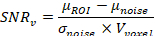. 2):
          (2)
       For the coil used here in combination with the reference solution, using Eq. 2 results in the following solution:
          (3)
       NOTE: When comparing the SNR of coils at different magnetic field strengths, the relaxation properties of the phantom need to be measured²³, unless a very long repetition time and very short echo time are used.
18. Check for susceptibility problems due to magnetic field inhomogeneities: load and run a multiple gradient-echo (MGE) sequence (Figure 7). Magnetic field inhomogeneities due to susceptibility differences are visible in the images with longer echo times, as the gradient echo does not refocus spins, which dephase due to static field inhomogeneities. This way, inhomogeneities in the sample may be visualized (due to air spaces in the sample), as well as B₀ field inhomogeneities introduced by the coil material. Use the following parameters, to be adjusted depending on the specifications of the spectrometer and coil used: TR 200 ms, TE 3.5 ms with 48 echoes spaced 3.5 ms apart, flip angle 30 degrees. Matrix size 128 x 128.
    NOTE: If multiple (potential) resonant modes or reflection dips were observed in the resonance (wobble) curve, repeat the above steps for each resonant mode to determine the most sensitive one. Depending on the microcoil, different parts of the microcoil assembly may be prone to unintended resonance modes.

5. High-resolution imaging

1. Run a 3D-FLASH experiment with the following parameters: TR 70 ms, TE 2.5 ms, matrix size of 128 x 64 x 64, FOV 1.6 x 0.8 x 0.8 mm, flip angle 30°, and receiver bandwidth 50 kHz.
2. Derive the pulse powers from the reference pulse power determined earlier; this is automatic in most imaging software. Determine the receiver gain using automatic adjustments. Adjust the FOV if necessary, covering the whole object in both phase-encoding directions to avoid aliasing. Run a gradient duty cycle simulation, if available on the system, to verify that the duty cycle of the experiment stays within the specifications of the gradient coils.
   NOTE: These parameters are specific to the coil used for demonstration; it is important to optimize to the local system specifics.

6. Recovering samples for further study or storage

1. Remove the sample capillary from the microcoil.
2. Using tweezers, remove the wax plugs under a stereomicroscope.
3. Use a syringe to wash the sample out of the capillary with a solution of choice. Alternatively, use a glass pusher rod to eject the sample.
4. To prevent dehydration of the sample, store in a suitable medium for storage.

Results

Coil Characterization
Upon successful tuning and matching of a coil, its performance may be characterized by the coil Q-factor, 90° reference pulse, and SNR/mm³. For the 1.5 mm ID susceptibility-matched solenoid coil demonstrated here, the measured Q-factor(unloaded) was 244, compared to 561 for a 5 mm birdcage coil.

The reference 90° pulse was 12 µs at a power level of 0.6 W; cf. 5 µs at 45 W for a 5 mm birdcage coil (Figure 4 and Figure 5). This equates to an RF pulse field strength (B₁), using of 0.53 mT for the microcoil and 1.17 mT for the birdcage coil¹⁴ where y is the gyromagnetic ratio, while tau is the pulse duration. Since the pulse power levels (P) differ, coils may be compared in terms of transmit efficiency : 0.69 mT/W^1/2 and 0.18 mT/W^1/2 for the microcoil and birdcage respectively¹⁴. Comparing by a 90° pulse, the microcoil is found to be a factor ≈ 4 times more sensitive than the birdcage coil.

Effect of susceptibility matching
At ultra-high field strengths, sample and coil susceptibility become a dominant factor for image quality, as seen in Figure 7A,7B. Compared to a coil lacking a susceptibility matching fluid reservoir, the signal is retained longer and more homogeneously in a reference sample. However, due to the susceptibility reservoir, the maximum sample dimensions decrease with respect to the coil without the reservoir.

High-resolution imaging
A high resolution of 13 x 13 x 13 μm³ of a Medicago truncatula root specimen was attained in 20 hours and 23 minutes (Figure 8). Starting from the surface of the root, the root cortex is seen, along with some residual water on the outside of the root. Furthermore, the xylem is observed as a dark band enclosing the phloem. Some air pockets are observed as dark spots with complete signal loss.

Symbiotic root nodules of M. truncatula may also be imaged using this protocol (Figure 9). Using a slightly larger unmatched coil (length circa 3500 µm, inner diameter 1500 μm), images with a resolution of up to 16 x 16 x 16 μm³ were obtained in 33 minutes.

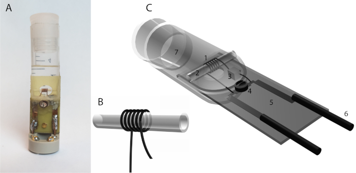
Figure 1: A solenoid microcoil. (A) The solenoid coil design consists of wire looped helically, typically wrapped around a capillary. The geometry of the wire, such as its thickness, diameter, number of windings, and wire spacing, influence the coil characteristics. (B) A home-built solenoid microcoil with a reservoir for susceptibility matching fluid (Fomblin). It consists of a 0.4 mm thick coated copper wire wound six times around capillary with an outer diameter of 1500 µm and a coil length of 3500 µm. The coil is submerged in a reservoir which is made from a syringe. Sample capillaries up to an outer diameter of 1000 µm can be inserted. Two capacitors are used, a 1.5 pF capacitor in series with the inductor and a second variable 1.5-6 pF capacitor is placed in parallel to the inductor. All components are soldered to a fiberglass board (yellow). It is mounted on a commercial holder (grey polymer) that is modified to support the reservoir.  (C) Solenoid coil design components: 1. solenoid coil, 2. sample capillary, 3. 1.5 pF tuning capacitor, 4. variable matching capacitor, 5. fiberglass base plate, 6. copper wire leads. Please click here to view a larger version of this figure.

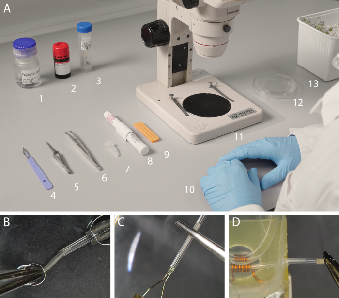
Figure 2: Sample preparation under a stereomicroscope. (A) Items needed for the preparation of microcoils. From left to right: 1. CuSO₄ reference solution, 2. perfluorodecalin, 3. microcoil, 4. scalpel, 5. positive tension tweezers, 6. tweezers, 7. capillaries outer diameter = 1000 μm, 8. wax pen, 9. capillary wax, 10. nitrile gloves, 11. stereomicroscope, 12. watch glass with Petri dish cover, 13. plant material in growth substrate. Not shown: 2 mL syringe with ø 0.8 x 40 mm needle and fine tissue paper. (B) Close up of sample insertion into a capillary using tweezers, while both are kept submerged. (C) Sealing of the capillary using molten wax. (D) Insertion of the prepared capillary into the microcoil. Please click here to view a larger version of this figure.

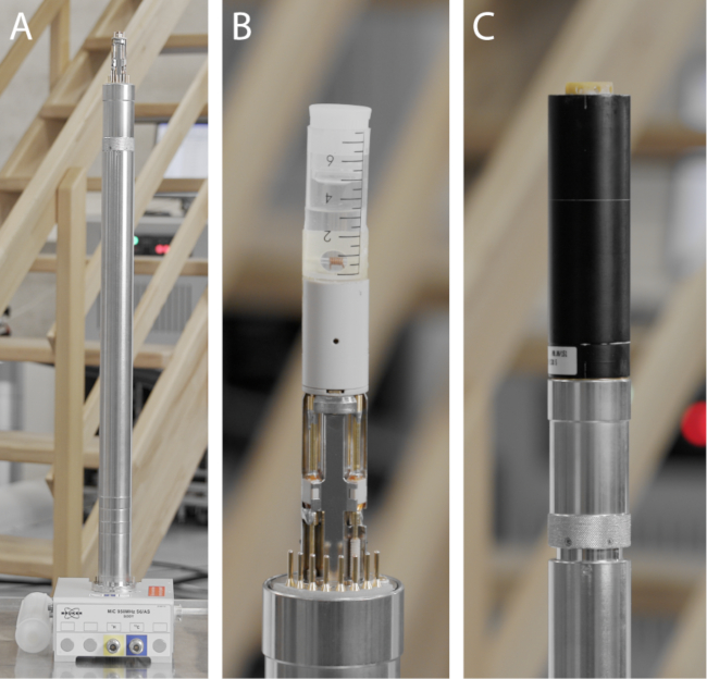
Figure 3: The component of a micro-imaging probe. (A) Micro5 probe base, containing all necessary connections for water cooling, heating, temperature sensors, gradient power, RF (co-axial connector visible) and optionally probe identification (PICS). Underneath the probe base are knobs that allow for adjusting the variable tuning and matching capacitors, as well as retaining screws to hold the probe in place inside the spectrometer. (B) The home-built microcoil mounting atop the probe-base. Note the variable capacitors (white ceramic) mounted on the probe-base that allow for tuning and matching. (C) Integrated 3-axial gradient mounted on the probe base with water-cooling receptacles and gold-plated contacts for grounding the gradient. Please click here to view a larger version of this figure.

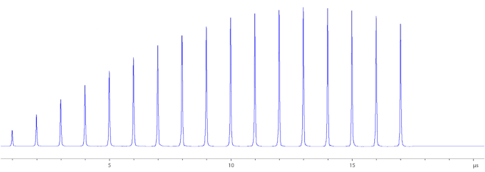
Figure 4: Nutation curve. A nutation curve is acquired to determine the reference pulse power. The reference pulse power (90° pulse) is defined as the combination of power and pulse length needed to generate a B₁ field that flips all available magnetization in the z-direction to the transverse plane. A series of a pulse is recorded in the absence of gradient encoding. With each pulse, either pulse length or pulse power is incremented. Here the pulse power is set to 0.6 W, while the pulse length is incremented by 1 µs each time. The maximum signal intensity indicates the 90° pulse, around 12 µs. The 180° pulse may also be determined in this way using the minimum intensity. Please click here to view a larger version of this figure.

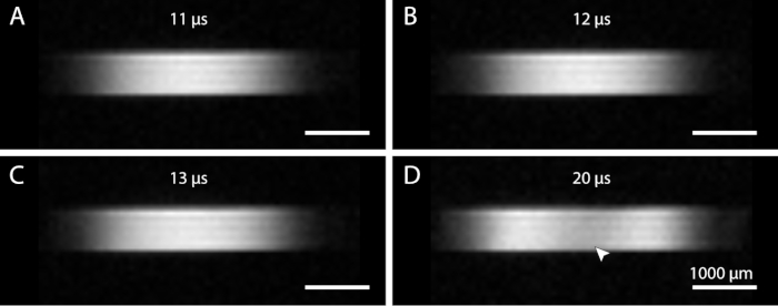
Figure 5: Visual determination of 90° pulse power. Once an approximate reference pulse power has been found using a nutation curve, it may be checked visually by varying the pulse length. Depending on the coil, the B₁ field may be more or less sensitive to changes. (A) 11 µs pulse length. (B) 12 µs pulse length, optimal for this coil. (C) 13 µs pulse length. (D) 20 µs pulse length. If the pulse power is set too high, over-tipping may occur, thereby reducing image intensity in the center of the coil (arrowhead). The increased B₁ field also increases the range of the coil, as can be observed in the width of the image. Please click here to view a larger version of this figure.

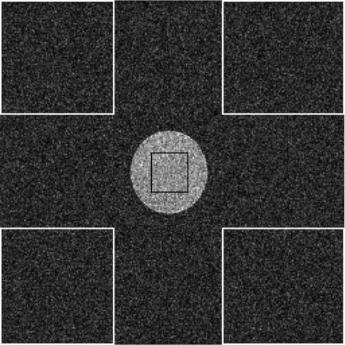
Figure 6: Region of Interest placement. The regions of interest (ROI) for the volume normalized SNR calculation can be seen. The mean sample intensity is taken from an ROI that falls within the reference solution sample. The mean noise and standard deviation are calculated from one or more ROI located in the corners of the image. Please click here to view a larger version of this figure.

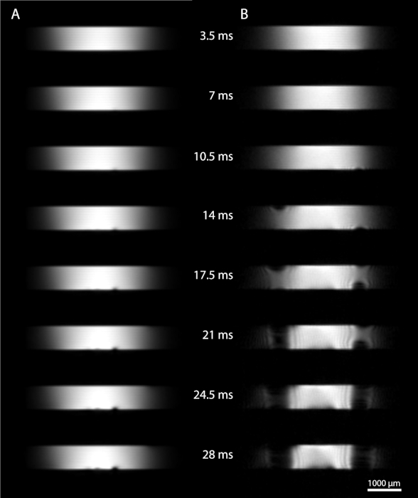
Figure 7: RF homogeneity evaluated by gradient echo imaging. A multiple gradient echo (MGE) sequence is used to evaluate RF (B­_1­ -Field) homogeneity using a series of gradient echoes. Basic parameters were: repetition time 200 ms, echo time 3.5 ms with the number of echoes 48, echo spacing 3.5 ms, 64 averages, acquisition time 27 m 18 s, flip angle 30°. Field of view was 5 x 5 mm, matrix 128 x 128, resolution 39 x 39 x 200 µm. (A) Susceptibility-matched coil. The susceptibility matching fluid (Fomblin) surrounding the RF coil reduces susceptibility effects due to the coil wire. Small air bubbles cause loss of signal as the echo time increases. (B) A coil (not susceptibility matched) with equal coil diameter. At longer echo times, increasing artifacts caused by B₀ field inhomogeneity are observed. Please click here to view a larger version of this figure.

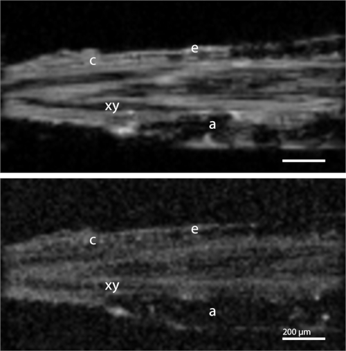
Figure 8: 3D imaging of a Medicago truncatula root section. (Top) FLASH image. Several features of the root section can be distinguished, including the epidermis (e), cortex (c), phloem (ph) and xylem (xy). Air pockets (a) in the root cause complete signal loss. Basic parameters were as follows: Repetition time 70 ms, echo time 2.5 ms, 256 averages, acquisition time 20 h 23 m. Resolution 13 x 13 x 13 µm³_­. Matrix size was 128 x 64 x 64 and field of view 1.6 x 0.8 x 0.8 mm. Receiver bandwidth 50 kHz. (Bottom) MSME image. Basic parameters were as follows: Repetition time 500 ms, echo time 5.2 ms, 28 averages, acquisition time 15 h 55 m. Resolution 13 x 13 x 13 µm³_­. Matrix size was 128 x 64 x 64 and field of view 1.6 x 0.8 x 0.8 mm. Receiver bandwidth 70 kHz. Please click here to view a larger version of this figure.

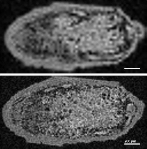
Figure 9: 3D imaging of a Medicago truncatula root nodule. (Top) Low-resolution image. Basic parameters were as follows: Repetition time 60 ms, echo time 2.3 ms, 4 averages, acquisition time 4 m. Resolution 31 x 31 x 31 µm³_­. Matrix size was 64 x 32 x 32 and field of view 2 x 1 x 1 mm. Receiver bandwidth 50 kHz. (Bottom) High-resolution image. Basic parameters were as follows: Repetition time 60 ms, echo time 2.3 ms, 8 averages, acquisition time 33 m. Resolution 16 x 16 x 16 µm³_­. Matrix size was 128 x 64 x 64 and field of view 2 x 1 x 1 mm. Receiver bandwidth 50 kHz. Please click here to view a larger version of this figure.

Discussion

This protocol is best suited to biological samples, as many materials and geological samples have significantly shorter T₂ relaxation times, which cannot be imaged by the sequences used here. Even some biological tissues, which exhibit high sample magnetic susceptibility heterogeneity, can be difficult to image at ultra-high field as the effects are correlated to the field strength²⁴. The protocol is not only useful for new coils but may also aid in troubleshooting and diagnosis of potential problems. When testing new or unknown samples, this protocol can be performed beforehand on the reference solution to verify that the experimental setup is functioning according to specifications. This aids in troubleshooting since the spectrometer can be excluded as a source of artifacts and malfunctions. In addition, this sets the tuning and matching capacitors on the probe to values typical for the microcoil.

When no signal is recorded upon the first experiment, the field of view of the localizer scan can be enlarged to check if the sample is seen. Next, recheck if the coil is tuned correctly and attempt another localizer scan. It is possible that the coil exhibits additional unintended resonant modes, in which case the correct one needs to be determined. If still no image can be obtained, remove the sample to check its position within the microcoil assembly and verify that the sample is intact (i.e., no air bubbles or leaks in the seals are present). Lastly, a sample may be prepared with water instead of PFD. In case the sample gives little detectable signal in the localizer scan, the surrounding water in the capillary can still be detected.

As microcoils are ideally very close to the sample, the magnetic susceptibility differences between the air and the wire can cause additional signal loss, as seen in Figure 7B. Potential artifacts include spatial mismapping and anomalous signal intensity variation. Especially gradient-echo type pulse sequences are affected by this non-uniform signal loss. For this reason, we presented a susceptibility-matched coil, by submerging the wire in fluorinert liquid (Fomblin or FC-43). The B₁ estimation method included in this protocol can help determine whether the B₁ susceptibility differences warrant the inclusion of susceptibility matching strategies in the design of the coil assembly. An alternative approach for constructing a susceptibility matched coil is to use susceptibility-matched wire²⁵. Furthermore, only susceptibility issues due to the coil are addressed with this approach. Susceptibility mismatches inside the sample (e.g., due to air spaces) remain challenging.

Air pockets or bubbles pose an experimental challenge that causes extensive signal loss, caused by susceptibility differences at the interface of the air and the fluid or specimen¹⁹ (Figure 5A). A critical aspect of successful sample preparation is the submersion of both sample and capillary. However, even small bubbles can cause signal losses, especially for gradient echo type sequences. Mobile air bubbles can migrate through the capillary until they are in contact with the sample. Some of these effects can be alleviated by slightly tilting the capillary so that one end is higher than the other. Tilting ensures potential air bubbles are held in place at the higher end, without disturbing the sample. It is also important to check that the capillary wax forms a good seal, as dehydration can cause large air bubbles to form.

For the air spaces inside the sample, PFD was used to fill up the intercellular air spaces while not penetrating the cell membranes²⁶. However, even with this approach, we were not able to remove all air spaces. Additionally, this approach means that we need an additional agent, which is usually not preferred due to the desire to study a system as noninvasively as possible.

The cylindrical shape of capillaries means that perfusion setups should be viable, especially for tissues vulnerable to decay, such as biopsies or studying processes in living root material. Two steps could realize a perfusion setup. First, connecting a medium feed tube as well as a drain tube at either side of the capillary would be sufficient to create a chemostat. Second, the addition of an indentation in the sample capillary could hold the sample in place against the direction of flow. This is analogous to a protocol published for planar microcoils¹⁰.

The noninvasive nature of MR imaging, combined with the inert liquid used in this protocol (PFD or Fomblin) means after completion of experiments, samples may be removed from their capillaries for further study. Combinations include optical or electron microscopy and other destructive imaging techniques. We have recently demonstrated a combination with optical microscopy on Medicago truncatula root nodules²⁷.

We have demonstrated a method for imaging plant material using dedicated microcoils on an ultra-high field NMR spectrometer. Relatively large sample volumes can be studied at high resolution with good RF homogeneity. Furthermore, spectroscopic imaging can be performed at higher resolutions than otherwise feasible. Adapting microcoil design to samples is facilitated by an efficient method to determine coil performance characteristics. The solenoid coil approach may also be readily applied to other samples than plants, including animal tissue. 

Materials

List of materials used in this article

Name	Company	Catalog Number	Comments
Reference solution preparation
CuSO4	Sigma-aldrich	469130	Crystalline powder for creating reference solution
D2O	Sigma-aldrich	151882	Liquid used to prepare reference sample
Weigh Scale	Sartorius	PRACTUM513-1S	Scale for weighing compounds
Sample preparation
Capillary 1000 μm (Outer diameter)	Hilbenberg GmbH	1408410	Sample capillaries
Capillary wax	Hampton Research	HR4-328	Solid wax used to seal samples
Disposable Scalpel	Swann-Morton	No. 11	Used to excise samples
Perfluorodecalin	Sigma-aldrich	P9900	Liquid used for submerging sample
Stereo Microscope	Olympus	SZ40	Tabletop binocular microscope
Syringe	Generic	-	Used to apply PFD and manipulate the sample
Vacuum Pump	Vacuubrand	MZ2C	Two-stage membrane vacuumpump used for removing air pockets from samples.
Wax pen	Hampton Research	HR4-342	Handheld wax pen used to melt and apply capillary wax to samples
Imaging Hardware
22.3 T Magnet	Bruker GmbH	950 US2	Narrowbore superconducting magnet
Air cooler	Bruker GmbH	-	Used to regulate probe temperature
Console	Bruker GmbH	Avance III HD	Controls operation of the spectrometer
Micro5 gradient coils	Bruker GmbH	Mic5	Removable gradient coils mount on the Micro5 probe body
Micro5 Probe body	Bruker GmbH	Mic5	Holds microcoils and gradient coils
RF microcoil	Home-built	-	contains Fomblin
Vector Network Analyzer	Copper Mountain Technologies	TR1300/1	Used to perform S11 reflectance test, frequency range 300kHz to 1.3 GHz
Water cooler	Bruker GmbH	BCU-20	Open loop watercooling to dissipate heat from gradient coil operation.