Culture and Assay of Large-Scale Mixed-Stage Caenorhabditis elegans Populations

Summary

To use Caenorhabditis elegans (C. elegans) in omics research, a method is needed to generate large populations of worms where a single sample can be measured across platforms for comparative analyses. Here, a method to culture C. elegans populations on large-scale culture plates (LSCPs) and to document population growth is presented.

Abstract

Caenorhabditis elegans (C. elegans) has been and remains a valuable model organism to study developmental biology, aging, neurobiology, and genetics. The large body of work on C. elegans makes it an ideal candidate to integrate into large-population, whole-animal studies to dissect the complex biological components and their relationships with another organism. In order to use C. elegans in collaborative -omics research, a method is needed to generate large populations of animals where a single sample can be split and assayed across diverse platforms for comparative analyses.

Here, a method to culture and collect an abundant mixed-stage C. elegans population on a large-scale culture plate (LSCP) and subsequent phenotypic data is presented. This pipeline yields sufficient numbers of animals to collect phenotypic and population data, along with any data needed for -omics experiments (i.e., genomics, transcriptomics, proteomics, and metabolomics). In addition, the LSCP method requires minimal manipulation to the animals themselves, less user preparation time, provides tight environmental control, and ensures that handling of each sample is consistent throughout the study for overall reproducibility. Lastly, methods to document population size and population distribution of C. elegans life stages in a given LSCP are presented.

Introduction

C. elegans is a small free-living nematode that is found throughout the world in a variety of natural habitats¹. Its relative ease of growth, fast generation time, reproduction system, and transparent body make it a powerful model organism that has been widely studied in developmental biology, aging, neurobiology, and genetics^2,3. The copious work on C. elegans makes it a prime candidate to use in -omics studies to comprehensively link phenotypes with complex biological components and their relationships in a given organism.

To use C. elegans in collaborative -omics research, a method is needed to generate large mixed-stage populations of animals where a single sample can be split and used across diverse platforms and instruments for comparative analyses. Creating a pipeline to generate such a sample requires keen awareness of diet, environment, stress, population structure, and sample handling and collection. Therefore, it is crucial to have standard and reproducible culturing conditions integrated into large-scale pipelines. In C. elegans research, two traditional methods are used to culture worms - agar Petri dishes and liquid culture⁴.

Historically, when large quantities of C. elegans are needed, they are grown in liquid culture⁴. The steps involved in generating a large population of worms in liquid culture require multiple handling steps that often include bleach synchronization to rupture gravid adult cuticles, releasing embryos to achieve the desired population size. However, when bleach synchronization is used, population growth is dependent on starting census size and, therefore, effects subsequent growth and population numbers. In addition, C. elegans strains vary in their cuticle sensitivity, exposure time, and stress response to bleach synchronization making it difficult to assay many strains at a time^5,6,7,8,9.

Additionally, worm growth in liquid culture requires a couple of transfer steps as it is often recommended to grow just one generation of worms before harvesting because overcrowding can easily occur if grown for multiple generations and lead to dauer formation despite the presence of food¹⁰. Dauer formation occurs through small signaling molecules such as ascarosides, often referred to as “dauer pheromones”^11,12,13,14, are released into liquid media and effect the growth of the population. Furthermore, growing large worm populations in liquid culture leads to excess bacteria accumulation in the culture, creating difficulties when a clean sample is needed for downstream phenotypic assays. Lastly, when a liquid culture becomes contaminated, it is more difficult to maintain as fungal spores or bacterial cells are easily dispersed throughout the media¹⁵.

The other traditional method of growing C. elegans is on agar Petri dishes. Commercially available Petri dishes allow one to easily grow multiple generations of mixed-stage worms without the rapid effects of overcrowding and high dauer formation as seen in liquid cultures. However, a disadvantage to worm growth on traditional agar Petri dishes is that the largest commercially available Petri dish does not yield large worm populations for an -omics study without adding in a bleach synchronization step. In summary, culturing mixed-stage populations of C. elegans on agar Petri dishes is more suitable for collecting -omics data, but we required a method to generate very large population sizes without liquid culturing.

Here, we present a method to culture and collect large mixed-stage C. elegans populations on large scale culture plates (LSCP). Collecting samples through this pipeline yields enough sample to gather phenotypic and population data, along with any data needed for -omics experiments (i.e., genomics, transcriptomics, proteomics, and metabolomics). In addition, the LSCP method requires minimal manipulation of the animals, less user prep time, provides tight environmental control, and ensures that handling of each sample is consistent throughout the study for overall reproducibility.

Protocol

1. Sterilize LSCP and equipment

1. Prepare glass LSCPs by handwashing, followed by dishwashing, and subsequent autoclaving to ensure glassware is free of contaminants before starting the experiment. Store autoclaved LSCPs in a clean dry location until in use.
   NOTE: Ensure LSCPs are dishwasher and autoclave safe. Ensure the LSCP lids are dishwasher safe.
2. Prepare LSCP lids by handwashing followed by dishwashing. Store LSCP lids in a clean bin until needed.
3. On the day Nematode Growth Media Agarose (NGMA) is prepped, wipe LSCP lids with 10% bleach solution twice, followed by 70% ethanol. Once wiped down with 10% bleach and 70% ethanol, keep LSCP lids in a clean bin in the laminar flow hood where the NGMA will be prepped.

2. Prepare nematode growth media agarose (NGMA)

1. Prepare NGMA by combining the following reagents into an autoclaved 2 L Erlenmeyer flask with stir bar on a stir plate: 2.5 g peptone, 3 g NaCl, 7 g agarose, 10 g agar, and 975 mL sterile water¹⁶. Ensure that the total volume equals 1 L. Tape a foil cap to the flask.
   NOTE: The preparation steps for the NGMA as described here will yield enough material for 2.5 LSCPs. The protocol can be tailored to the needed LSCP batch size in a given experiment.
2. Autoclave on liquid cycle at 121 °C and 21 p.s.i. for 45 min.
3. Turn on the water bath and set to 50 °C. Bring the autoclaved NGMA to the water bath to cool to 50 °C.
4. Bring 2 L Erlenmeyer flask of NGMA into the hood or cleaned space and set on a stir plate. Use a thermometer to track NGMA temperature.
5. After the NGMA has reached 50 °C, add the following in the order listed with a sterile disposable pipette inside the hood or cleaned space: 25 mL of 1 M KH₂PO₄ (K phosphate buffer), 1 mL of cholesterol (5mg/mL in ethanol), 1 mL of 1 M CaCl₂, 1 mL of 1 M MgSO₄, 1 mL of nystatin (10mg/mL), and 1 mL of streptomycin (100 mg/mL)¹⁶.
6. Pour 400 mL of NGMA into a sterile glass LSCP, approximately 1.3 cm deep, allow the LSCP to solidify on flat surface in the hood and place the autoclaved foil lid back on the LSCP.
7. Once agar is set, remove the foil, and place a clean air-tight lid onto LSCP and move to 4 °C for storage. Store NGMA in LSCPs at 4 °C until in use and use within 5 days.

3. Generate E. coli food for NGMA on LSCP

1. To generate a stable food source, generate batches of HT115 (DE3) E. coli using a small batch averaging concept consistent with the central limit theorem¹⁷. Store at -80 °C. When needed pull E. coli bacterial stock(s) from -80 °C to thaw¹⁸.
   NOTE: In this protocol, E. coli bacterial stocks were grown in a bioreactor. At the end of the culture growth, the culture was diluted 1:50, and the measured OD₆₀₀ was 0.4. Thus, the culture had an effective OD₆₀₀ of 20. Bacteria were pelleted, weighed, and resuspended in K medium at a concentration of 0.5 g/mL (wet weight), transferred into 2 mL aliquots, and frozen¹⁹.

4. Bacterial lawn on NGMA

1. Bring NGMA LSCPs out of 4 °C to room temperature (RT) for several hours before spreading the bacterial lawn to allow the entire LSCP to reach RT.
2. Pull out needed E. coli bacterial stock(s) from -80 °C to thaw¹⁸.
3. Dilute E. coli bacterial stock(s) with 2 mL of sterile K-medium to achieve 0.5 g E. coli in 4 mL per NGMA LSCP. Carefully pipette 4 mL of E. coli in the middle of the NGMA LSCP.
4. Use a sterile spreader to spread bacteria into a rectangle leaving approximately 3.8 cm of room around the edges of the NGMA E. coli free.
5. Leave the NGMA LSCP with E. coli in the hood with the fan on for 1 h to ensure the E. coli suspension fully dries.
6. Once the bacterial lawn is dry, push the lid on tightly and store at 4 °C until used.

5. Chunk worms to reduce stress and age variability across samples

1. Streak worms from a frozen worm stock to a newly seeded 6 cm plate⁴. This plate will serve as the “master chunk” plate.
   NOTE: Chunking is an optimal method to transfer worms from a homozygous strain²⁰. If a strain is heterozygous or needs to be maintained by picking and mating, chunking is not advisable. Chunking frequency may need to be optimized depending on worm genotypes used, temperature chosen for growth, and downstream steps.
2. After the master chunk plate is full of healthy gravid adults (approximately 3 days) with plenty of E. coli lawn still present, follow standard C. elegans chunking guidelines as described in WormBook to produce four total chunk plates⁴.
3. Store all chunk plates in a controlled temperature (CT) room at 20 °C unless otherwise specified for growth.
   NOTE: If users of this protocol do not have access to a CT room as described here it is recommended to use either a small incubator where the temperature can be controlled or a designated room where environmental conditions can be controlled as much as possible. If neither of these alternate options are available, note that variation in sample growth may be greater.
4. Once many gravid adults are observed in the 4^th chunk plate, move on to Step 6.

6. Spot bleaching gravid adults onto LSCP

NOTE: This bleaching technique is used to eradicate most contaminants and dissolve the cuticle of the hermaphrodites releasing embryos from the adult worm. The bleach solution will soak into the NGMA prior to the embryos hatching.

1. Bring LSCPs out to RT for several hours prior to spot bleaching worms.
2. Prepare a 7:2:1 ratio of ddH₂O : bleach : 5 M NaOH. Make this alkaline hypochlorite solution fresh just before use.
   NOTE: Use the same stock of bleach and NaOH throughout the duration of a given experiment to avoid bleach batch affects. Bleach used in this protocol was 5-10% sodium hypochlorite.
3. Light a Bunsen burner and flame a worm pick before proceeding. Scoop fresh E. coli onto a sterile pick from the edge of the bacterial lawn on the LSCP.
4. Pick a single gravid adult from the 4^th chunk plate for spot bleaching.
5. Pipette 5 μL of the alkaline hypochlorite solution into one corner of the LSCP away from the E. coli lawn.
6. Place the picked gravid adult into the 5 μL alkaline hypochlorite solution. Tap the nematode to help disrupt the cuticle and release eggs.
7. Repeat steps 6.4 – 6.6 for a total of 4x and place 5 gravid adults evenly around the E. coli lawn. Pick all 5 gravid adults from the same 4^th chunk plate to ensure nearly genetically isogenic individuals are added to a given sample.
8. Place the lid back onto the LSCP.
9. Repeat steps for all LSCPs.

7. Worm growth in controlled temperature (CT) room

1. Following spot bleaching, place the lid tightly onto the LSCP and place in the CT room set to 20 °C with constant airflow and a 12L:12D photoperiod (12 h light and 12 h darkness).
2. Note the time and position where the sample was placed in CT room.
   NOTE: Position within the room should always be documented to record any environmental differences that samples that could potentially encounter while growing. Once the sample is in the CT room, it should remain in its assigned spot undisturbed. Do not open the lid of the LSCP in the CT room to decrease the chance of contamination.
3. Take the LSCP to a microscope, outside of the CT room, to observe the population growth and density.
   NOTE: Each C. elegans strain and sample will vary in its growth, so monitor samples closely. While it is recommended to not disturb the growth of the LSCP while in the CT room, LSCPs were transported out of the CT room and lids were opened every 2 days to monitor sample growth. Taking the sealed lids off the LSCPs every 2 days also allows for O₂ to flow into the LSCP.
4. Before harvesting ensure that the LSCP has become full of a large population of worms. Use the following criteria to decide if the LSCP is ready to be collected.
   1. Ensure that the LSCP is full of gravid adult worms.
   2. Ensure that the plate contains a large population size (i.e., worms cover the entire surface of the agar).
   3. Ensure that the plate does not have many eggs on the surface of the agar (i.e., the maximum number of worms should have hatched).
   4. Ensure that the plate has minimal to no E. coli left, indicating that the worms would starve and generate dauer larvae if left on the plate for an additional two days.
      NOTE: Although most LSCPs are ready to harvest between 10 to 20 days, depending on strain and sample, check each LSCP frequently upon establishing this protocol to determine normal harvest times.
5. Clean gloves and area with 70% ethanol between handling LSCPs to avoid cross contamination between strains.

8. Harvesting the LSCP sample

1. Turn on and allow the centrifuge to cool to 4 °C prior to harvesting samples.
2. Prepare three 50 mL conical tubes with 50 mL of M9 solution per LSCP to be harvested.
3. Label one 15 mL conical tube per LSCP.
   NOTE: All centrifugation steps are performed in the 15 mL conical tube, because worms tend to pellet well in these tubes.
4. Pour 50 mL of M9 solution (from one 50 mL conical tube in Step 8.2) onto the LSCP surface and swirl around to ensure that M9 covers the entire NGMA surface.
5. While M9 sits on the LSCP surface, prime a sterile serological pipette with M9.
   NOTE: By priming the sterile serological pipette with M9 this ensures that less worms stick to the inside of the plastic pipette, preventing sample loss.
6. Tilt the LSCP so M9 and the worm population gather in one corner of the LSCP.
   NOTE: The mixture of M9 solution and worms from the LSCP will be referred to as the “worm suspension” in downstream steps.
7. Using a primed serological pipette with an automatic pipettor, pipette worm suspension and place into the original 50 mL conical tube. Once 50 mL of worm suspension is collected, place the conical tube on a rocker to disrupt bacteria clumps and debris.
8. Repeat steps 8.4 - 8.7 collecting 150 mL of worm suspension per LSCP.
9. Transfer 15 mL of worm suspension, from one of the three 50 mL conical tubes, by pouring into a labeled 15 mL conical tube set aside in step 8.3. Centrifuge the 15 mL conical tube at 884 x g for 1 min at 4 °C. The majority of worms will pellet at the bottom of the tube.
10. Aspirate off the supernatant ensuring to not disturb the worm pellet.
11. Continue adding approximately 13 mL of worm suspension to the same 15 mL conical tube repeating steps 8.9 and 8.10 until all 150 mL of worm suspension are consumed. Invert the tube and disturb the pellet between centrifugations to wash and aspirate off as much bacteria and debris as possible.
    NOTE: At this step, the contents from all three 50 mL conical tubes are condensed in a single 15 mL tube.
12. Add 10 mL of clean M9 to the 15 mL conical tube and agitate the worm pellet by inverting. Centrifuge the 15 mL conical tube at 884 x g for 1 min at 4 °C. Aspirate off the supernatant ensuring to not disturb the worm pellet. Repeat twice.
    NOTE: If there is a great amount of debris or bacteria in sample, repeat step 8.12 until the sample is clean.
13. Once the sample is clean, add ddH₂O to the worm pellet for a total of 10 mL of ddH₂O and worms. Agitate the worm pellet by inverting. Move quickly into step 9.1, as worms must remain in ddH₂O for 5 min or less to avoid osmotic stress.
    NOTE: Suspending worm pellets in ddH₂O is the preferred solvent for downstream -omics steps. Worms can be suspended in other solvents or buffers if they are compatible with a given experimental workflow.

9. Estimate population size

NOTE: Move through Steps 9.1 – 9.7 quickly. The mixture of ddH₂O and worms from step 8.13 are referred to as the “worm sample” in subsequent steps.

1. Prior to pipetting the worm sample, prime pipette tip to be used with M9 to avoid worms sticking to the inside of the plastic pipette preventing sample loss and reducing count variation.
2. Take a 100 μL aliquot of worm sample and dilute it into 900 μL of M9. Mix well and make a serial dilution (1:10, 1:100, 1:1000). Repeat this step twice to achieve a total of three sets of aliquot replicates.
   NOTE: Pipetting worms can cause high variability in sample population counts. Ensure that the worm sample is homogenous prior to pipetting the desired aliquot.
3. Set the 15 mL conical tube on a rocker to continue moving culture while aliquots are counted.
4. Ensure the worm sample is well mixed and homogenous. Pipette 5 μL from the 1:10 worm sample, dispense it onto a microscopy slide, and count the number of worms. If this number is less than approximately 50 worms, then also count the 1:100 and 1:1000 dilutions. If it is more than 50, move to the next serial dilution.
   NOTE: If too many worms cannot be accurately counted, use the next serial dilution for counting instead.
5. Count each aliquot replicate of each dilution 3x. At the end of counting, for most cultures, 9 total counts will be documented (i.e., 3 total counts for each aliquot replicate).
6. Average the dilution counts to determine the estimated population size of the worm sample. These dilution counts will determine the volume of worm sample needed to create desired aliquot size for -omics steps.
   NOTE: In this experiment, aliquots of approximately 200,000 mixed-stage worms were generated. In addition, one aliquot of approximately 50,000 mixed-stage worms was set aside for sorting in a large particle flow cytometer (described in Step 10).
7. Once the worm sample has been split into appropriate aliquots, flash freeze in liquid nitrogen and store the sample at -80 °C.
   NOTE: Do not freeze the aliquot intended for large particle flow cytometry.

10. (Optional) Prepping sample for large particle flow cytometry

NOTE: Steps 10, 11, and 12 are the authors’ preferred method to record sample growth (i.e., population size and population distribution of C. elegans life cycle stages) and determine success of a culture. Users of this protocol can substitute optional Steps 10, 11, and 12 with their own metrics of growth success. Steps 10, 11, and 12 are described here for two reasons; first, so users who have equipment used in Steps 10, 11, and 12 can replicate these steps and second, to show validation of this growth method. Step 9 above provides a good estimation of total number of worms to determine aliquot sizes, and step 10 is a more quantitative metric to estimate the number and population distribution of worms in a given sample.

1. Bring the aliquot of approximately 50,000 mixed-stage worms (set aside in Step 9.6) up to 10 mL total volume in M9 solution.
2. Make a solution composed of 1 mg/mL of E. coli and a 1:50 dilution of 0.5 μM red fluorescent microspheres¹⁹.
3. Add 200 μL of this solution to the 10 mL of mixed-stage worms in M9 and incubate while rocking for 20 min.
4. After 20 min, centrifuge the 15 mL conical tube at 884 x g for 1 min at 4 °C.
5. Aspirate off the supernatant ensuring to not disturb the worm pellet.
6. Wash the worm pellet twice with M9 solution to eliminate excess bacteria and red fluorescent microspheres.
7. Add 5 mL of M9 to the worm pellet and ensure that the pellet looks clean. If the pellet is clean, add 5 mL of M9 with 50 mM sodium azide to both straighten and kill the worms for accurate counting and sizing²¹.
8. Document time and date when sodium azide is added to sample.
9. Set the sample aside on rocker until needed for large particle flow cytometry.
   NOTE: Sodium azide is known to affect nematode physiology (i.e., body length, metabolism, and thermotolerance). Therefore, it is critical to note the time worms are exposed to sodium azide as many of these physiological affects happen within a matter of minutes²². Due to the known physiological effects of sodium azide on worms, this treatment will affect downstream image quality and should be considered.

11. (Optional) Documenting population distribution and prepping 384-well plate for imaging

NOTE: Step 11 uses a large particle flow cytometer (LPFC). Basic knowledge of a LPFC is assumed in this protocol. Other methods can be substituted to document the growth and population distribution of samples. Steps documented here are for users who plan to use a LPFC in their pipeline²³.

1. Turn on, clean and prime the LPFC, and allow laser(s) to warm for 1 h prior to sorting samples.
2. After the laser has warmed, open the “Histogram” profile and scale to a Time of Flight (TOF) of 2050.
3. Add a bar region to the “Histogram” spanning a TOF range of 100. The first bar region covers a TOF of 50-150.
4. Continue to create twenty bar regions each spanning a TOF range of 100. These bar regions will span the entire TOF range from 50 – 2050. See Supplementary Table 1 for the exact gated regions to use across the TOF distribution.
5. Save this Histogram set up as an “Experiment” to use in future LPFC runs.
6. Select calibrated 384-well plate or calibrate instrument to a 384-well plate to dispense objects into.
7. Once in the calibrated 384-well plate template, set template to dispense 20 gated objects into four wells (four technical replicates of each gated region) for each of the 20 bar regions created during Steps 11.3-4. See Supplementary Table 2 for an example layout of how to dispense worms into the 384-well plate.
8. Transfer sample from step 10.9 into a 50 mL conical tube and add additional M9 solution to achieve approximately 40 mL total volume.
9. Start automatically sorting the sample per the parameters set in step 11.7 while continuously stirring the sample to prevent settling and simultaneously dispensing objects from the sample into the calibrated 384-well plate.
   NOTE: Ensure the flow rate of the LPFC is operating between 15-20 objects per second and specify no doubles to be sorted.
10. Once entire sample has been sorted and the maximum number of gated regions have been dispensed into the 384-well plate, take the sample off LPFC and clean instrument.
    NOTE: When larger TOF regions are reached, it may become challenging to continue to fill the 384-well plate due to low event counts in that TOF region. Fill as many of the gated regions as possible to get the best idea of where C. elegans life-stages fall within the LPFC distribution prior to running out of sample.
11. Place a sealing film on top of the 384-well plate until imaged.
    NOTE: Image plate as quickly as possible after sorting because samples are treated with sodium azide²². Red fluorescent microspheres can be seen in the collected LPFC data files (i.e. PH Red data in output text file) based on the level of red fluorescence emitted in each sorted object to help identify which objects are alive worms, dead worms, dauers, or junk²⁴.

12. (Optional) Imaging 384-well plate

NOTE: Step 12 uses a plate-reading micro confocal microscope. Basic knowledge of a micro confocal microscope is assumed in this protocol. Other methods can be substituted to document the growth and population distribution of samples.

1. Using a plate-reading micro confocal microscope with a 20x lens.
2. Open the “Objective and Camera” tab and set to “10x Plan ApoLambda” mode.
3. Open the “Camera Binning” tab and set to “2”.
4. Open the “Sites to Visit on Plate” tab and set to “4” sites per well and “overlap sites 10%” to later stitch together images.
5. Open “Wavelength” tab and set to “Brightfield 1”.
6. Open “Illumination” tab and set to “Transmitted light, bright sample”.
7. Place the 384-well plate in the microscope and set the “Z Stack” to “Calculate Offset” and find the proper focal plane for the samples in the 384-well plate.
8. Run the 384-well plate on the micro confocal microscope collecting four images per well.
9. Montage the four images together to create one image per well.

Results

Growth of C. elegans using the LSCP method yields an average of approximately 2.4 million mixed-stage worms per sample over 12.2 days. Growth of C. elegans using the LSCP method enables users to generate large mixed-stage populations of C. elegans with little handling and manipulation of the animals, which is ideal for large-scale -omics studies (Figure 1). Once a LSCP has become full of adult worms, reached a large population size, and has minimal bacteria left, users can harvest and estimate the population size. This point can also serve as a quality control by evaluating whether the population is sufficient to use in an -omics pipeline (Figure 2). Population dynamics are dependent on the strain itself, behavior of the strain (i.e., burrowing strains tended to have lower worm recovery), and growth success (i.e., contamination). The LSCP method was tested on 15 strains of C. elegans containing a mixture of Caenorhabditis Genetics Center (CGC) mutants and Caenorhabditis elegans Natural Diversity Resource (CeNDR) wild strains²⁵. Strain genotypes are described in Supplementary Table 3.

The LSCP method yielded population sizes from approximately 94,500 to 9,290,000. The mean population size within the reference strain, PD1074, and across strains was approximately 2.4 million worms (Figure 3). No significant differences were found in estimated population sizes between C. elegans strains over the course of an average of 12.2 LSCP growth days (Figure 4). PD1074 LSCPs took between 10 – 14 days to grow to a full mixed-stage population. The mean growth time across PD1074 was 10 days. The slowest growing strain grew for a maximum of 20 days, and the fastest growing strain grew for a minimum of 10 days (Figure 4).

Therefore, using this LSCP method, users can easily integrate new strains of interest into a study with little knowledge of developmental timing and background expertise. Note that strains and phenotypes that have to be maintained by picking, have fecundity defects, are heterozygous, or have growth defects may not work well in this pipeline.

Large particle flow cytometry and imaging of samples allows users to document population distribution. A wide variety of platforms can be used to measure successful population growth.

For reproducible -omics measurements, it is important to grow consistent cultures. The metrics of culture reproducibility are number of worms and a consistent size distribution for a given strain. We show the sample distribution for the reference strain, PD1074 – a variant of the original N2 Bristol strain, using the LPFC^23,26 and micro confocal microscope images as proxies for growth success. As worms were measured from the L1 stage through gravid adult on the LPFC distribution (Figure 5), subsequent imaging (Figure 6), and the variation in the population distribution across samples (Figure 7), we can see that this pipeline generated a mixed-stage population of C. elegans.

To take a closer look at the population distribution of our mixed-stage samples, we looked at the distribution of 35 PD1074 LSCPs by looking at the percent of worms that fall within each region across the entire Time of Flight (TOF) (i.e., body length) distribution (Figure 7A,B).

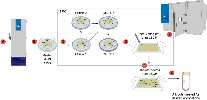
Figure 1: Overview of the LSCP worm growth pipeline. (A) Once received in the lab, all strains were prepared and frozen for long-term storage at -80 °C². (B) A “master chunk” plate was prepared from a frozen worm stock and stored at 15 °C to be used for no longer than one month. (C) Each sample went through four successive chunking steps to reduce generational stress prior to growing on the LSCP. (D) 5 individual gravid adults were picked from the “chunk 4” 6 cm plate in Step (D) and spot bleached on five given areas of the LSCP. (E) The LSCP was placed in a Controlled Temperature room and grown at 20 °C until the LSCP was full of adult worms, reached a large population size, and had minimal bacteria left. (F) The worm population was harvested and collected for downstream steps. (G) Aliquots were created from the LSCP and were flash frozen for downstream desired applications. Please click here to view a larger version of this figure.

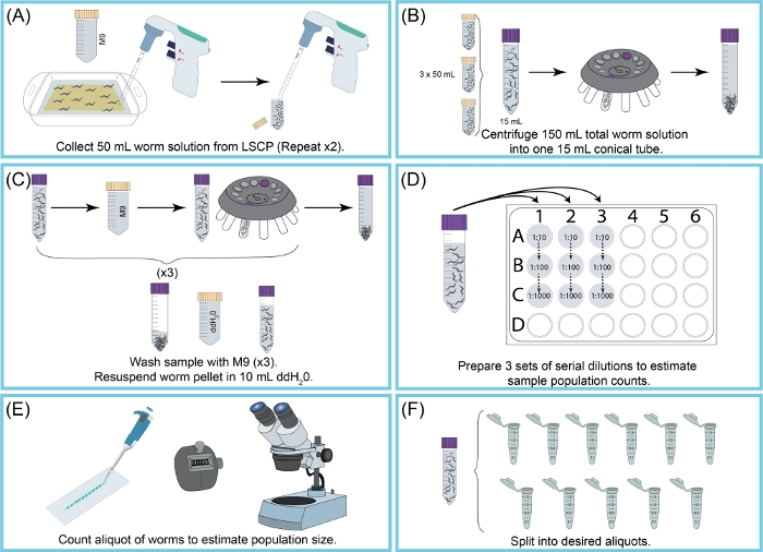
Figure 2: Overview of LSCP harvesting and estimating population size. (A) 50 mL of M9 were used to wash worms off the NGMA surface. Worm suspension was pipetted into a 50 mL conical tube. Step (A) was repeated twice. (B) 15 mL of worm suspension was poured into a new 15 mL conical tube. Worms were pelleted by centrifuging. M9 + debris were aspirated off without disturbing worm pellet. Step (B) was repeated until all 150 mL of worm suspension were collected. (C) The worm pellet was washed and centrifuged three times with M9 to eliminate remaining debris. Once the sample was clean, the worm pellet was resuspended in 10 mL of ddH₂O. (D) A serial dilution of the sample was created to estimate worm population size. The dilution factor(s) that allowed worms to be counted accurately were used. The dilution factor(s) used changed depending on the population size of the LSCP. (E) Once the dilution factor(s) were chosen, all worms from all three aliquot replicates of that dilution were pipetted onto a clean slide and worms were counted under a dissecting microscope. (F) Sample was split into appropriate-sized aliquots. Please click here to view a larger version of this figure.

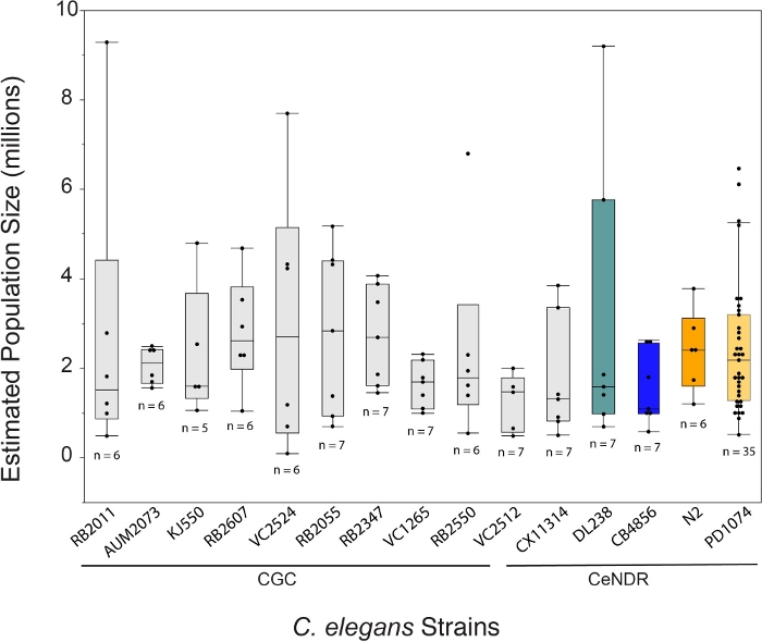
Figure 3: LSCP method generated on an average a population of 2.4 million mixed-stage worms. The LSCP yields population sizes in the smallest population growths at around 94,500 and at the biggest population growths at around 9,290,000. The mean population size across all strains was 2.4 million worms. Bars underneath C. elegans strain names indicate whether a strain is a CGC mutant or CeNDR natural isolate. LSCP sample size is displayed for each strain. Comparisons for all pairs using Tukey’s HSD Test were performed. No significant differences were observed between estimated population sizes across C. elegans strains (F(14,108) = 0.7, p = 0.77). Colored bars indicate standard color displays for respective C. elegans strain representation. Please click here to view a larger version of this figure.

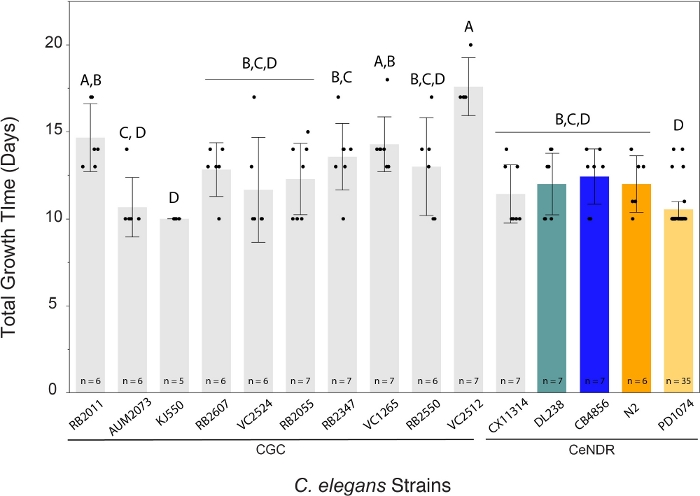
Figure 4: LSCP method generated large mixed-stage populations of worms in 10 – 20 days. A given C. elegans LSCP grew until the sample was full of adult worms, reached a large population size, and had minimal bacterial lawn left. LSCPs took between 10 – 20 days to grow to a full mixed-stage population, depending on the strain. The mean growth time across the strains was 12.2 days. LSCP sample size is displayed for each strain. Each error bar was constructed using 1 standard deviation from the mean. Levels not connected by same letter are significantly different. Comparisons for all pairs using Tukey’s HSD Test. A significant difference was found in the amount of growth time on LSCP needed across C. elegans strains (F(14,108) = 8.8, p < 0.0001*). Colored bars indicate standard color displays for respective C. elegans strain representation. Please click here to view a larger version of this figure.

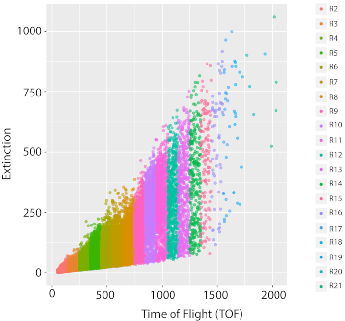
Figure 5: Mixed population and growth measurement of the wild-type reference strain, PD1074. A representative LPFC distribution of one LSCP growth of the wild-type reference strain, a variant of the original N2 Bristol strain, (PD1074) documents the size distribution and event counts of a mixed-stage population. The x-axis displays the length (Time of Flight, TOF) of the worms sorted. The y-axis displays the optical density (optical extinction, EXT) of the worms sorted. Each data point is a worm that was documented in the sample. Each TOF region that was used for image analysis is displayed in a different color. Twenty TOF regions were created (R2 – R21) ranging from a TOF of 50 to 2050. Details on each TOF region can be found in Supplementary Table 1. Please click here to view a larger version of this figure.

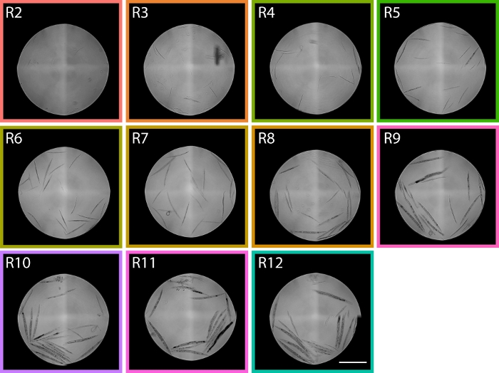
Figure 6: Images of worms sorted from TOF regions ranging from R2 – R12 show the PD1074 LPFC distribution. In region R2, L1 worms can be identified and in region R9 predominately gravid adults are identified, spanning the two developmental larval extremes giving us approximate regions within the flow cytometer distribution of where stages are expected in the distribution. Scale bar represents 1 mm. Representative images were taken from the LPFC distribution displayed in Figure 5, and the colored boxes correspond to regions from Figure 5. Please click here to view a larger version of this figure.

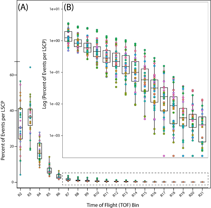
Figure 7: Population distribution across time of flight (TOF) regions in the wild-type reference strain, PD1074. Distribution of worms across the entire TOF region showing the regions where worms were found. Each PD1074 LSCP is represented as an individual color. (A) The x-axis shows the twenty TOF regions (R2 – R21) observed and counted for the LSCP, displaying the entire size distribution. The y-axis shows the percent of worms from a given LSCP that had a body size that fell into a given TOF region. (B) As a smaller fraction of the worm population falls between the R7-R21 regions, the log of the percent of worms that fell within each region was taken to display the population distribution. The x-axis displays the R7-R21 TOF regions. The y-axis displays the log of the percent of worms from a given LSCP that had a body size that fell into a given TOF region. Please click here to view a larger version of this figure.

Supplementary Figure 1: Mean daily temperature (°C) of growth conditions under which the LSCP was grown and handled. Reported temperatures of the Controlled Temperature (CT) room were documented and collected throughout the six-month span of sample growth and collection. The average daily temperature is reported here. No significant differences were observed between the temperature in which the LCSP grew during the duration of the project (F(5,24) = 2.59, p = 0.0524). The entire temperature difference spanned no greater than 0.003 °C throughout the six-month duration of sample growth and generation. Please click here to download this figure.

Supplementary Table 1: TOF gated regions used to sort worms into 384-well plates for imaging. Binned regions were created to span a TOF of 100 across the entire TOF distribution from 50 – 2050. Gated regions can be changed and optimized to suit your needs. Each TOF region that was used for image analysis is displayed in a different color. Please click here to download this table.

Supplementary Table 2: 384-well plate template of TOF regions and replicate layout. Every sample was sorted into a 384-well plate for imaging. Four replicates were created for each region selected for sorting. Gated regions can be changed and optimized to suit your needs. See Supplementary Table 1 for specific gated regions created and used in this protocol. Each TOF region that was used for image analysis is displayed in a different color. Please click here to download this table.

Supplementary Table 3: C. elegans strains used in this protocol contain a mixture of CGC and CeNDR strains. The strain, genotype, strain source, and details are described in this table. Please click here to download this table.

Discussion

A variety of vessels can be used as a LSCP. In this protocol, a standard glass baking dish was used. The LSPCs in use had outer dimensions of 35.56 x 20.32 cm, inner dimensions of 27.94 x 17.78 cm, and approximately 4.45 cm deep and came with a fitted lid. Thus, the amount of bacteria used here has been optimized for a LSCP with the above dimensions to yield a large population of mixed-stage worms. Bacterial volume and concentration can be adjusted to fit the experimental needs.

Contamination by mold, fungi, or other bacterial sources can occur at any step in the LSCP method, so handle samples with care. Prior to starting any step in the protocol, ensure that the working space is cleaned with 70% ethanol and 10% bleach. If available, treat used areas with UV light for 30 min and turn on a HEPA air-filter 30 min prior to starting each step.

By growing the LSCP in a controlled setting (i.e., in a CT room set at 20 °C), the user can more easily track the growth of the sample and document potential contamination. If the surface of the LSCP becomes contaminated, either cut out the contamination when possible and let the sample continue to grow or discard the sample if the contamination is not possible to control. It is imperative to address contamination quickly to reduce unwanted growth and to ensure it is not outcompeting worms for resources.

This method is meant for those who want to grow large-scale mixed-population cultures of C. elegans. Although it may be possible to grow synchronized populations of worms on the LSCP as done on commercially available Petri dishes and in liquid culture, the authors have not tested this option. Additionally, if users wish to grow more than approximately 2.4 million worms on average in a given sample, a different method is recommended⁴. Growth success is dependent on the strain being processed in the pipeline. The authors were able to successfully grow populations of approximately 2.4 million worms in at least five biological replicates of 15 C. elegans strains, indicating that the method is robust.

Prior to starting the experiment note that the age and health of a given worm can influence fecundity and subsequent population growth time. Ensure that worms are maintained in healthy conditions with minimal stress prior to being used in this pipeline. It is assumed that stock samples have been created, frozen, and kept at -80 °C to reduce genetic drift over time.

Depending on the needs of a given experiment, the number of starting gravid adults on a LSCP can be changed. Altering the number of starting gravid adults on the LSCP will change the growth rate and thus time to harvest. Five gravid adults are used to seed each LSCP for the following reasons: (1) A simple, fast, and efficient way to seed many C. elegans strains onto LSCPs at one time was needed and (2) to reduce the age differences amongst the gravid adults picked that could lead to the growth heterogeneity.

This method allows the user to harvest large populations of worms with all life cycle stages present. With current methods available, collecting large-scale samples of C. elegans requires bleach synchronization to obtain the number of worms desired for downstream work. Given this approach, one can now grow as many worms as previously possible in fermenters or large-scale liquid cultures without the difficulties associated with bleach synchronizing and multiple handling steps. Our protocol allows one to target strains of interest efficiently, use minimal handling time in growing the sample itself, and isolate stages of worms or the population as needed in downstream pipelines.

A LPFC was utilized as a tool to document the population distribution and size in a given LSCP. The LPFC used is a continuous flow system that analyzes, sorts, and dispenses worms based on their size (TOF) and optical density. As a given worm passes through the flow cell, the axial light-loss detector captures the amount of signal light blocked by a 488 nm-solid state laser for the length of time it takes a worm to pass through, giving the user the TOF and optical density of the worm. Fluorescence collection optics and detectors can also be utilized to maximize fluorescence sensitivity and collection on each sample. LPFC collection parameters will vary based on instrument. Users can employ a variety of platforms to capture worm size and are not limited to using this protocol if a LPFC is not available.

The authors are using samples grown in the method described here to identify unknown metabolites in various strains of C. elegans via Liquid Chromatography – Mass Spectrometry, NMR spectroscopy, and RNA sequencing. The authors plan to continue to use this method for growth of samples in this pipeline with a variety of C. elegans strains as new strains of interest can be easily processed using this pipeline.

Materials

List of materials used in this article

Name	Company	Catalog Number	Comments
10 mL Sterile Serological Pipettes	VWR	89130-898
10 ul pipette tips	VWR	89079-438
100 ul pipette tips	VWR	89079-442
1000 mL Graduated Cylinder	VWR	10124-380
1000 ul pipette tips	VWR	89079-488
15 mL conical tubes	VWR	89039-668
190 Proof Ethanol	VWR	89125-166
2 L Wide Neck Erlenmeyer Flask	VWR	75804-654
50 mL conical tubes	VWR	75874-294
Agar	Sigma	05040-100G
Agarose	Sigma	A9539-500G
BVC Control G Fluid Aspiration System	Vacuubrand
Calcium Chloride	Sigma	449709-10G
Cholesterol	Sigma	C3045-25G
Clorox Bleach	VWR	89414-502
Conviron Control Temperature Room	Conviron		https://www.conviron.com/environmental-rooms
Corning Low Volume 384 Well Black with Clear Flat Bottom Polystyrene TC-Treated Microplate	VWR	89089-866
Fisher Scientific Accuspin 3R	Fisher
Flat-Bottom 24-Well Plate	VWR	29443-952
Honeywell True HEPA Purifier 465 sq ft.	Home Depot	204390560
HT115 E. coli (DE3)	CGC	HT115(DE3)	https://cgc.umn.edu/strain/HT115(DE3)
Kimwipes	VWR	470224-038
Large Scale Culture Plate (LSCP)	Pyrex	1090948	Pyrex 2-quart Glass Baking Dish with Red Lid
Magnesium Sulfate	Sigma	C86677-25G
MgSO4	VWR	97062-998
Microscope Plain Slides	VWR	16004-422
Millipore Filter	Millipore	1.11727.2500
Molecular Devices ImageXpress	Molecular Devices	Model Number:IXMConfocal	https://www.moleculardevices.com/products/cellular-imaging-systems/high-content-imaging/imagexpress-micro-confocal#gref , Authors used MetaXpress Software Version 6.5.4.532
Nystatin (10mg/mL)	Sigma	N6261-25MU
Peptone	Sigma	P7750-100G
Petri Dishes (6 cm)	VWR	25384-092
Pipette Controller	VWR	613-4180
Potassium Chloride	Fisher	P217-3
Potassium Phosphate Monobasic	VWR	0781-500G
Potasssium Hydroxide	Fisher	P250-500
Red Fluroscent Microspheres	Polysciences	19507-5
Sodium Chloride	Sigma	746398-500G
Sodium Hydroxide	Fisher	111357
Sodium Phosphate Dibasic Anhydrous	Fisher	BP332-500
Standard Gilson Pipette Set	Gilson	FA10002M, FA10004M, FA10006M
Streptomycin (100mg/mL)	Sigma	S6501-25G
Union Biometrica COPAS BioSorter	Union Biometrica		https://www.unionbio.com/biosorter/ , authors used: Flow Pilot software version 1.6.1.3.

References

- Félix, M. A., Braendle, C. The natural history of Caenorhabditis elegans. Current Biology. 20 (22), 965-969 (2010).
- Corsi, A. K. A Transparent window into biology: A primer on Caenorhabditis elegans. WormBook. , 1-31 (2015).
- Brenner, S. The genetics of behaviour. British Medical Bulletin. 29 (3), 269-271 (1973).
- Stiernagle, T. Maintenance of C. elegans. WormBook: The Online Review of C. elegans Biology. , https://www.ncbi.nlm.nih.gov/books/NBK19649/ (2006).
- Xiong, H., Pears, C., Woollard, A. An enhanced C. elegans based platform for toxicity assessment. Scientific Reports. 7 (1), 9839(2017).
- Loer, C. M., et al. Cuticle integrity and biogenic amine synthesis in Caenorhabditis elegans require the cofactor tetrahydrobiopterin (BH4). Genetics. 200 (1), 237-253 (2015).
- Li, Y., Paik, Y. K. A potential role for fatty acid biosynthesis genes during molting and cuticle formation in Caenorhabditis elegans. BMB Reports. 44 (4), 285-290 (2011).
- Meli, V. S., Osuna, B., Ruvkun, G., Frand, A. R. MLT-10 Defines a Family of DUF644 and Proline-rich Repeat Proteins Involved in the Molting Cycle of Caenorhabditis elegans. Molecular Biology of the Cell. 21 (10), 1648-1661 (2010).
- Fritz, J. A., Behm, C. A. CUTI-1: A novel tetraspan protein involved in C. elegans CUTicle formation and epithelial integrity. PloS One. 4 (4), 5117(2009).
- Golden, J., Riddle, D. A pheromone influences larval development in the nematode Caenorhabditis elegans. Science. 218 (4572), 578-580 (1982).
- Jeong, P. Y., et al. Chemical structure and biological activity of the Caenorhabditis elegans dauer-inducing pheromone. Nature. 433 (7025), 541-545 (2005).
- Srinivasan, J., et al. A blend of small molecules regulates both mating and development in Caenorhabditis elegans. Nature. 454 (7208), 1115-1118 (2008).
- Kaplan, F., et al. Ascaroside Expression in Caenorhabditis elegans Is Strongly Dependent on Diet and Developmental Stage. PLoS One. 6 (3), 17804(2011).
- Çelen, İ, Doh, J. H., Sabanayagam, C. R. Effects of liquid cultivation on gene expression and phenotype of C. elegans. BMC Genomics. 19 (1), 562(2018).
- Andersen, E. C., Bloom, J. S., Gerke, J. P., Kruglyak, L. A Variant in the Neuropeptide Receptor npr-1 is a Major Determinant of Caenorhabditis elegans Growth and Physiology. PLoS Genetics. 10 (2), 1004156(2014).
- Rosenblatt, M. A central limit theorem and a strong mixing condition. Proceedings of the National Academy of Sciences. 42 (1), 43-47 (1956).
- Boyd, W. A., Smith, M. V., Freedman, J. H. Caenorhabditis elegans as a model in developmental toxicology. Methods in Molecular Biology. 889, 15-24 (2012).
- Nika, L., Gibson, T., Konkus, R., Karp, X. Fluorescent Beads Are a Versatile Tool for Staging Caenorhabditis elegans in Different Life Histories. Genes, Genomes, Genetics. 6 (7), 1923-1933 (2016).
- Stiernagle, T. Maintenance of C. elegans. , Available from: http://www.wormbook.org/chapters/www_strainmaintain/strainmaintain.html (2020).
- Denver, D. R., Morris, K., Streelman, J. T., Kim, S. K., Lynch, M., Thomas, W. K. The transcriptional consequences of mutation and natural selection in Caenorhabditis elegans. Nature Genetics. 37 (5), 544-548 (2005).
- Massie, M. R., Lapoczka, E. M., Boggs, K. D., Stine, K. E., White, G. E. Exposure to the metabolic inhibitor sodium azide induces stress protein expression and thermotolerance in the nematode Caenorhabditis elegans. Cell Stress & Chaperones. 8 (1), 1-7 (2003).
- Kevin, S., Pulak, R. Techniques for Analysis, Sorting, and Dispensing of C. elegans on the COPAS Flow-Sorting System. C. elegans. Methods in Molecular Biology. Strange, K. 351, Humana Press. 275-286 (2006).
- Lee, D., et al. Selection and gene flow shape niche-associated variation in pheromone response. Nature Ecology & Evolution. 3 (10), 1455-1463 (2019).
- Cook, D. E., Zdraljevic, S., Roberts, J. P., Andersen, E. C. CeNDR, the Caenorhabditis elegans natural diversity resource. Nucleic Acids Research. 45, 650-657 (2016).
Reprints and Permissions
Request permission to reuse the text or figures of this JoVE article
Request Permission