ARL Spectral Fitting as an Application to Augment Spectral Data via Franck-Condon Lineshape Analysis and Color Analysis

Summary

This protocol introduces Franck-Condon Lineshape Analyses (FCLSA) of emission spectra and serves as a tutorial for the use of ARL Spectral Fitting software. The open-source software provides an easy and intuitive way to perform advanced analysis of emission spectra including excited state energy calculations, CIE color coordinate determination, and FCLSA.

Abstract

The ARL Spectral Fitting application provides a free, publicly accessible, and fully transparent method for performing Franck-Condon Lineshape Analysis (FCLSA) on spectral data, in addition to CIE color coordinate determination and basic spectral processing. While some of the features may be found in commercial software or in programs made by academic research groups, we believe that ARL Spectral Fitting is the only application that possesses all three of the aforementioned attributes.

This program is intended as a standalone, GUI-based application for use by an average laboratory researcher without requiring any coding knowledge or proprietary software. In addition to the standalone executable hosted on ARL GitHub, the associated MATLAB files are available for use and further development.

FCLSA augments the information found in luminescence spectra, providing meaningful insight into the relationship between the ground and excited states of a photoluminescent species. This insight is achieved by modeling spectra with two versions (modes) of an equation that are characterized by either four or six parameters, depending on which mode is used. Once optimized, the value of each of these parameters can be used to gain insight into the molecule, as well as to perform further analysis (for example, the free energy content of the excited-state molecule). This application provides tools for easy by-hand fitting of imported data, as well as two methods for optimizing this fit-damped least-squares fitting, powered by the Levenberg-Marquardt algorithm, and derivative-free fitting utilizing the Nelder-Mead simplex algorithm. Furthermore, estimations of sample color can be performed and reported in CIE and RGB coordinates.

Introduction

Photoluminescence measurements, comprising both fluorescence and phosphorescence spectra, are widely used throughout various academic fields and industrial applications¹. Photocatalysts are increasingly used in organic synthesis for the production of complex and valuable target molecules^2,3,4. In order to determine the energetics of photocatalysts, the excited state energy is routinely estimated using emission spectra. The development of novel lighting materials, such as organic light emitting diode (OLED) luminophores, necessitates that the observed color output be characterized and reported^5,6. Commission international de l'éclairage (CIE) color coordinates are routinely used for this purpose⁷.

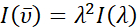
The purpose of the ARL Spectral Fitting application is to provide a quick and easy method to augment spectral data through meaningful analysis that is widely accessible both in terms of ease-of-use and availability (https://github.com/USArmyResearchLab/ARL_Spectral_Fitting). This software performs several routine spectral processing functions automatically for the user, including data normalization and conversion between wavelength, λ, and wavenumber, , units with appropriate intensity scaling as shown in the equation below¹. The software is capable of handling a variety of input and output file formats. Several advanced analyses are easily performed using the software such as the calculation of CIE and chromaticity coordinates, color prediction, determination of the excited state free energy (ΔG_ES) in various units, and FCLSA for the determination of the FCLSA parameters⁸.

A graphical user interface (GUI)-based application was pursued because it allows any researcher to perform this analysis and requires no background knowledge of computer science. This application was written in MATLAB, using its App Designer tool. Outside of ARL Spectral Fitting, finding a publicly-accessible implementation of an application designed to perform Franck-Condon Lineshape Analysis is practically impossible. This is because research groups do not publicly release their implementations, preferring instead to keep them proprietary.

Franck-Condon Lineshape Analysis (FCLSA) is often used in the photophysical characterization of novel compounds because of the rich information it conveys about the molecule^{9,10,11,12,13,14}. Each of the four parameters (six if in double mode) gives information about the excited state of the molecule. The energy quantity, or 0-0 energy gap, (E₀) is the difference in zeroth energy levels of the ground and excited states of the molecule. The full width at half maximum (Δv_½) informs about the widths of individual vibronic lines. The electron-vibrational coupling constant, or Huang-Rhys factor, (S) is a dimensionless calculation based on the equilibrium displacement between ground and excited states of the molecule¹⁵. Finally, the quantum spacing parameter (ħω) is the distance between vibrational modes that govern the nonradiative decay of a molecule.

The equations for single and double mode FCLSA are as follows:

where the parameters are as previously defined. In the double mode equation, S and ħω are separated into medium (_M) and low (_L) energy terms. is the intensity at the wavenumber v^10,16,17,18. In both equations, the summation is performed over N quantum levels with a default value of N = 5, as is commonly used in the literature¹¹, but any integer can be specified in the ARL Spectral Fitting Software under Settings | Fit.

Protocol

1. Data import

1. To import data, press the Import Data button. Select the type of spectrum being imported-either excitation or emission.
   1. Once a spectrum type is chosen, ensure that the MATLAB file explorer will appear. From this window, select the desired file and press Open. Supported file types include .TXT, .CSV, .XLS, and .XLSX.
      NOTE: Some data processing is performed automatically before plotting the imported data. This includes: detection of x-axis units (wavenumber or wavelength) and conversion to wavenumber, if appropriate; intensity normalization of the highest peak to 1; calculation of the energy quantity, if appropriate; and estimation of the quantum spacing. These values are calculated based on detected data peaks with energy quantity assigned to the wavenumber value of the highest energy peak and quantum spacing based on the averaged distance between vicinal peaks, which necessitates the detection of at least two peaks.
2. To load any of the pre-packaged sample spectra, press the button corresponding to the desired spectrum, found under Info | Sample Spectra. Nine sample spectra come pre-packaged with the application.
3. To load and plot more than one spectrum at a time, activate the check box Allow multiple data spectra on axes under Settings | General | Figure Settings.
4. To select a different loaded spectrum than is currently active, press the Select Spectrum to Fit button and then choose the desired spectrum from the list shown on the newly visible Select Spectrum panel.

2. Data processing

NOTE: The user may wish to perform data processing prior to the fitting process. Available processes include:

1. Selection of a peak to act as a basis for normalization: To select a peak to act as the basis for intensity normalization, press the Select peak for normalization button found under Settings | General. Follow the instructions shown on screen. The default peak for intensity normalization is the highest intensity peak found during import.
2. Conversion between x-axis units: To convert the x-axis's units between wavenumber (cm^-1) and wavelength (nm), toggle the slider found under Settings | X-Axis to the desired mode (either Wavenumber or Wavelength). Intensity as well as x-axis units will be adjusted for all loaded spectra, using the equation given above.
3. Constraining of x-axis range: To manually constrain the x-axis range, select Manually adjust X-axis and fit limits under Settings | X-Axis. Then, use the revealed controls to specify the x-axis range. By default, the application will automatically expand and contract the x-axis range to fit all loaded data points.
4. Alternative E₀ calculation methods: To select an alternative calculation method for the energy quantity, select the desired method found under Settings | Fit. The default method is Full FCLSA fit. To change to another method, select the corresponding radial button and follow onscreen instructions¹⁹.

3. Manual fitting

NOTE: Based on the amount of structure visible in the spectrum, it may be highly advantageous to initialize the fitting parameters with appropriate estimates prior to optimization. This initialization can decrease the time required for optimization and helps to ensure that the values returned by optimization are realistic for the spectrum.

1. Plot the fit function with its current parameter values by pressing the Plot Fit Function button.
2. Using a combination of the coarse and fine adjustment buttons, sliders, and edit fields, adjust parameter values to increase the goodness of fit for loaded data. By default, the coefficient of determination (R²) is displayed in the upper-left-hand corner of the graph. Use this as a quantitative measure of the goodness of fit to guide the choice of parameter values.
   NOTE: Because the energy quantity (E₀) and quantum spacing (ħω) are calculated by the application upon data import, it is recommended that these values be held constant or minimally varied when fitting by-hand.
3. By default, this application utilizes the single mode Franck-Condon Lineshape Analysis formula as it is most relevant for room temperature spectra. If desired, such as when fitting 77 K spectra, toggle between the single and double mode in Settings | Fit.
   NOTE: Overparameterization becomes a larger issue when fitting in double mode as opposed to single mode due to the increased number of free-floating parameter values. Broad, structureless emission spectra pose the largest issue to the fitting algorithms and may result in cross-correlation between FCLSA parameters, particularly between Δv_½ and S. When fitting spectra, it is imperative that the obtained FCLSA parameters are verified to be physically realistic using literature precedence as a guide.

4. Optimization

1. After satisfactory initial parameters are found, further optimization can be performed. To do this, press the blue Optimize Fit button. Optimization will run and replot the fit function with newly optimized parameter values.
2. Two optimization options are provided: the least-squares and simplex methods. To switch between these two methods, toggle to the desired method in Settings | Optimization.
3. If desired, customize the optimization method using the settings found under Settings | Optimization.
   NOTE: In order to provide the user with control over the optimization routines, the following customization options are possible for both optimization methods:
   1. Fix a parameter’s values: To fix a parameter’s value during optimization, press the check box in the edit field corresponding to the desired parameter.
   2. Custom bounding of a parameter during optimization: To reveal the custom bounding options, activate the Allow custom parameter bounding during optimization check box in Settings | Optimization. To specify custom bounds for a parameter’s value during optimization, use the controls revealed by pressing the Custom bounds button under the edit field corresponding to the desired parameter.
   3. Custom end triggers for optimization: To adjust the maximum number of iterations, termination tolerance on model value, or termination tolerance on coefficient values, activate the corresponding check box in Settings | Optimization and enter the desired value into the corresponding edit field.
      NOTE: The following customizations are available only for the Least-Squares optimization:
   4. Goodness-of-fit statistics: To display goodness-of-fit statistics (degree-of-freedom adjusted coefficient of determination, sum of squares due to error, degrees of freedom in the error, and root mean square error) after optimization is complete, activate the check box found under Settings | Optimization.
   5. Robust fit options: To activate robust fit options, select the desired menu from the dropdown list under Settings | Optimization. By default, this option is off. If desired, activate Least Absolute Residual or Bisquare Weights fitting, which give lower weight to outlier data points.
   6. Threshold data weighting: To preferentially weigh data points above a threshold intensity, choose an intensity to act as a threshold and a weight multiplier to apply to all points above that threshold. By default, this option is set to on, and threshold and weight multiplier are set to 0.1 and 1.2, respectively. These options are available in Settings | Data Weighting.
   7. Extrema data weighting: To preferentially weight data points surrounding local extrema (peaks and valleys), select the number of data points surrounding each extremum to apply the preferential weights to, as well as what the weight multiplier should be for those points. These points are more feature rich as they are directly associated with the fitted parameters. Look for extrema data weighting settings under Settings | Data Weighting which is set to on as a default setting, and the number of points and weight multiplier are set to 5 and 5, respectively. To visually identify which data points are used in the preferential weighting, select Fill salient data points.

5. Chromaticity and free energy calculations

1. Ensure that the optimized fit of the data and the associated parameter values are satisfactory before proceeding to additional calculations. To perform these calculations, press the Calculate button, located at the bottom of the Calculations pane.
   NOTE: The first value returned, labeled ΔG_ES (cm^-1), is the free energy of the excited state calculated using the equation shown below. The default unit for this value is inverse centimeters (cm^-1), but units of electronvolt (eV) and joule (J) are also available. The calculation for free energy of the excited state is given by the equation
   
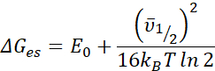
   1. To change the unit, select the desired option from the dropdown list box found under Settings | Calculations. This value is determined based on the energy quantity (E₀), full width at half-max (Δv_½), Boltzmann constant (k_B), and environmental temperature of the experiment (T). The value for experimental temperature is assumed to be 298 K but can be specified as 77 K or any other temperature²⁰.
      1. To change the experimental temperature, choose the desired option under Settings | Calculations | Experimental Temperature.
         NOTE: The second value returned is the CIE chromaticity coordinate, calculated from the currently selected spectrum. When plotted on a chromaticity diagram, this value shows the predicted color of the active data spectrum.
   2. To display the chromaticity diagram with coordinate plotted, press the pop-out button (represented by a square with an arrow pointing towards the upper-right-hand corner) next to the Chromaticity Coordinate text box.
   3. To check for the predicted color of the sample, use the third calculation, shown as a colored rectangle. This estimation is based off the same calculation that yielded the chromaticity coordinate. By default, CIE Standard Illuminant D65 is used to make this prediction. To change the illuminant, select the desired option from the dropdown menu labeled White Point in Settings | Calculations.
2. To calculate CIE chromaticity coordinates and color values for multiple loaded spectra simultaneously, activate the corresponding checkbox found under Settings | Calculations.
   NOTE: This setting is on by default. Once a second spectrum is plotted, the icon on the pop-out button next to the Chromaticity Coordinate label will change from the square with an arrow pointing to the upper-right-hand corner to three dots (· · ·).
   1. Press the · · · button to reveal a panel labeled Select Spectra. Select the desired spectra from this panel and choose to Export Values as a table and/or Display Diagram to reveal the chromaticity diagram with all coordinates plotted and labeled.

6. Data export

1. Once again, ensure that the fit of loaded data is satisfactory, and that all desired calculations have been performed. To export both loaded and calculated data, press the Export Data button. There are six data export options: Figure, Parameter Values, Spectrum Data Points, Fit Data Points, Color Values, and Chromaticity Diagram.
   1. To export the displayed plot as a figure pre-formatted for publication or presentation, select Figure. This formatting can be disabled under Settings | General | Figure Settings. Supported file types include .EPS (vector-graphics file), .JPG, .PNG, and .PDF.
   2. To export all parameter values—with or without calculated values—as a table, select Parameter values. Inclusion of calculated values is toggleable under Settings | Calculations and supported file types are .CSV, .TXT, .DAT, .XLS, and .XLSX.
   3. To export data of the currently selected spectrum as a series of x-y data points, select Spectrum data points. x-values will use either wavenumber (cm^-1) or wavelength (nm) units, depending on how the graph is defined via the settings. Supported file types are the same as above in 6.1.2.
   4. To export the fit as a series of x-y data points, again dependent on the current mode of the axes, select Fit data points. Supported file types are the same as above in 6.1.2.
   5. To export chromaticity and CIE coordinates as well as the predicted color as an RGB value, if enabled, select Color Values. Supported file types are the same as above in 6.1.2.
   6. To export the chromaticity diagram with the chromaticity coordinates plotted on it associated with the loaded spectrum, select Chromaticity Diagram. Supported file types are .EPS, .JPG, .PNG, and .PDF.

Results

Using the fitting routine described above, Franck-Condon Lineshape Analysis was performed on two spectra that come pre-packaged with the application: the room temperature (292 K) and low temperature (77 K) emission spectra for 9,10-diphenylanthracene dissolved in toluene. Measurements were obtained using a spectrofluorometer with fluid solutions in 1 cm cuvettes and a standard cuvette holder for room temperature measurements. The low temperature measurements were obtained by immersing NMR tubes into liquid nitrogen in a dewar to generate frozen glass samples. All spectra were corrected for the detector response. A single mode fit was sufficient for the room temperature spectrum, while double mode was used to model the low temperature spectrum. Color analysis was performed on both spectra and found to yield similar estimates.

To fit the room temperature spectrum, by-hand adjustment was used after least-squares optimization with default customizations. The final parameter values obtained were as follows: E₀ = 24380 cm^-1, Δv_½ = 1200 cm^-1, S = 1.25, ħω = 1280 cm^-1. The resulting coefficient of determination calculated was 0.99947 as shown in Figure 1. Calculation of free energy of the excited state using these parameter values yielded a value of 25,000 cm^-1.

Simplex optimization was used to fit the low temperature spectrum. By-hand adjustment was not necessary after optimization. The final parameter values obtained were as follows: E₀ = 24764 cm^-1, Δv_½ = 746 cm^-1, S₁ = 1.13, ħω₁ = 1382 cm^-1, S₂ = 0.31, ħω₂ = 651 cm^-1. The resulting coefficient of determination calculated was 0.9991 as shown in Figure 2. Calculation of free energy of the excited state using these parameter values yielded a value of 25,700 cm^-1.

Color analysis of the low temperature spectrum yielded the following results: chromaticity coordinate = [0.15819, 0.03349], CIE coordinate = [0.19571, 0.041432, 1], and predicted RGB value = [67, 0, 233]. The values obtained for the room temperature spectrum were very similar to that of the low temperature spectrum with unperceivable color differences.

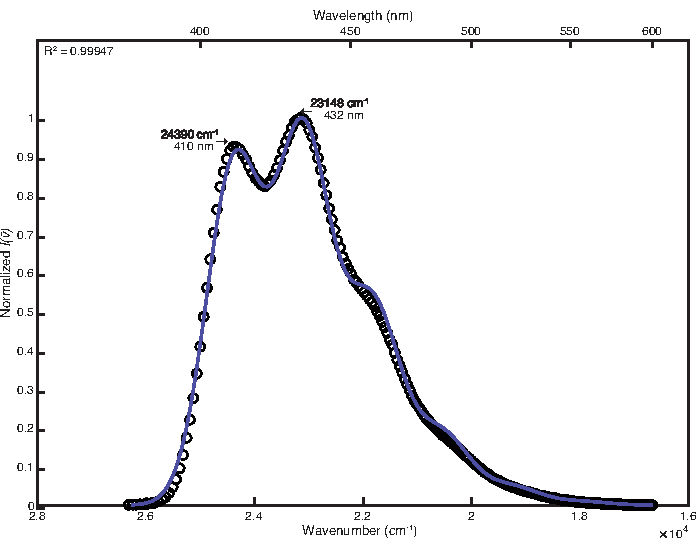
Figure 1: Single mode fit of 9,10-diphenylanthracene (292 K): This figure shows the room temperature emission spectrum of 9,10-diphenylanthracene and its FCLSA fit function, achieved through least-squares optimization followed by by-hand adjustment of parameter values. This is an example of a loosely structured spectrum. Please click here to view a larger version of this figure.

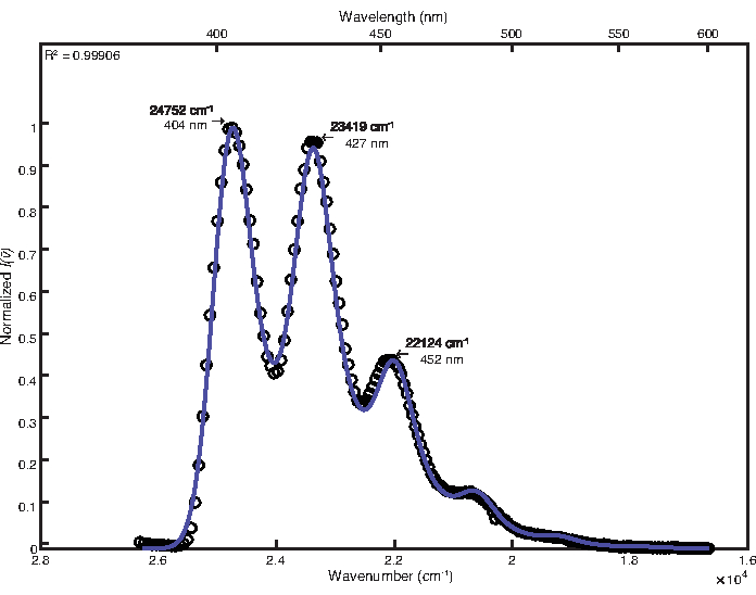
Figure 2: Double mode fit of 9,10-diphenylanthracene (77 K): This figure shows the low temperature emission spectrum of 9,10-diphenylanthracene and its FCLSA fit function, achieved through a simplex optimization. This is an example of a highly structured spectrum. Please click here to view a larger version of this figure.

Discussion

This application provides an easy and rapid analysis of emission spectra through two main methods commonly used in the photophysical community. The first is Franck-Condon Lineshape Analysis (FCLSA), which gives insight into the energetics and vibronic coupling associated with decay of excited state molecules back to their ground states. This is achieved by optimizing parameter values to maximize the goodness of fit of a spectrum using one of two possible FCLSA modelling equations. The second method of analysis provides insight into the observed color of the light emitted from the molecule. By combining tristimulus color curves with provided intensity data, the CIE coordinate can be calculated. This determination allows for the highly accurate color prediction of both absorption and emission spectra.

Experimental photoluminescence spectra are commonly measured using a photomultiplier tube (PMT) or charge coupled device (CCD) as a detector and plotted as emission intensity versus wavelength (nm). Many photophysical characterizations, including FCLSA and calculation of the free energy of the excited state, are performed in wavenumber space, as demonstrated by the use of (cm^-1) in the corresponding equations above. In addition to the x-axis conversion, the emission intensity as measured versus wavelength, denoted as I(λ) must be converted to . This application automatically identifies the original x-axis units of imported spectral data as either wavelength (nm) or wavenumber (cm^-1). By default, the application then converts the spectral data, normalizes the spectrum to unity at the maximum intensity peak, and plots the spectrum as "Normalized vs. wavenumber (cm^-1)" to indicate that the correct intensity conversion was applied. Although it is recommended that all fitting be performed using wavenumber units, the application can also plot the spectrum as "Normalized I(λ) vs. wavelength (nm)" by following the instructions in section 2 above.

There are two optimization algorithms available for use in the application. The default option is damped least-squares, which utilizes the Levenberg-Marquardt algorithm²¹. Combining a version of gradient descent and the Gauss-Newton algorithm, this algorithm finds local, not necessarily global, minima. While this is a significant limitation, the algorithm offers advantages in its customizability-this method can take into account preferential weighting of data points, perform robust fitting, and display advanced goodness-of-fit statistics²². The alternative method of optimization is derivative-free, powered by the Nelder-Mead simplex algorithm²³. This algorithm uses a heuristic method to return a global minimum of the given cost function (in this case, a sum of squared differences between predicted and observed intensities). The simplex method has been used for FCLSA before, though the code implementing it was never published²⁴.

Both the least-squares and simplex optimization methods work best for structured spectra that exhibit narrow, well defined, and symmetric peaks. As spectra become less structured, meaning that they lose symmetry and the peaks broaden, these methods lead to less robust fits where parameters can become highly correlated. Typically, spectra recorded at low temperatures or in rigid media are more structured compared to those obtained near room temperature or in fluid solution^12,25,26. The robust fit options included with the least-squares method can help to alleviate this issue. This problem can be significantly diminished if one or more of the parameters are fixed to a constant value during optimization. For instance, IR spectroscopy experiments can be used to determine relevant quantum spacing (ħω) values. Alternatively, relevant literature values can be used to set custom bounds for the parameters.

In some instances, the FCLSA fit, and parameters obtained from the optimization routines do not adequately represent the data even when robust fit options or fixed parameters are employed. This is a failure of the fitting algorithms and may be associated with the multiple FCLSA fitting parameters (potential overparameterization) or spectral shape of the data (featureless spectra). In these cases, further improvement of the fits may be obtained using a "by-hand fit" of the data with manipulation of the FCLSA parameters. The adequacy of such fits can be assessed visually and quantified by comparing goodness-of-fit statistics that are automatically included in the plot.

A general routine to follow for an accurate by-hand fit consists of the following five steps: First, determine an initial estimate for E₀ manually or automatically using one of the three methods provided. By default, the parameter's value is assigned to the wavenumber associated with the highest intensity peak detected upon data import. Alternatively, the user can define E₀ as the wavenumber at which the emission spectrum intersects its corresponding excitation spectrum. The final method to determine E₀ uses the so-called X% Rule, where X = 1 or 10. In this method, E₀ is assigned to a wavenumber X% of the full width at half-maximum (FWHM) intensity of the most prominent data peak assuming a Gaussian band shape. The second step in the by-hand fitting protocol is to calculate ħω based on quantum spacing observed in the structure of the emission spectrum. If possible, refer to the IR spectrum of the molecule and try to correlate the photoluminescence-based value to a strong band in the IR spectrum. Third, determine S based on the relative intensities of spectral peaks. Fourth, determine a rough Δv_½ based on bandwidth. Fifth, iteratively readjust S and Δv_½ as necessary.

The difficulty with performing FCLSA using broad, relatively featureless spectra was demonstrated through the fitting procedure for 9,10-diphenylanthracene in fluid solution at 292 K compared to that performed for the more structured spectrum obtained in frozen glass at 77 K. When fitting the room temperature spectrum, optimization returned an initial coefficient of determination of 0.9971 that was improved to 0.9994 through by-hand tuning of the parameters and visual inspection of the results. In contrast, by-hand fitting of the low temperature variant was unnecessary due to the fine structure of the spectrum that resulted in a coefficient of determination equal to 0.9991 after simplex optimization.

In many instances, both optimization routines (least-squares and simplex) return very similar results. This is indicative of them finding a global minimum for the FCLSA parameters. In general, the least-squares method tends to be better suited to data that is noisy, is not well structured, or contains many near-zero data points at the spectrum’s tails. Conversely, the simplex method tends to return better fits than the least-squares method for data that is well structured and possesses few outlier points. In these cases, the simplex method typically requires little by-hand pre-optimization of parameter values and no adjustment after optimization. For those cases in which the data’s noise or overall lack of structure prevents a high-quality fit using either of the provided optimization methods, it is recommended that the by-hand fitting method (see above) be employed with no subsequent optimization.

This application offers several advantages over previous implementations of Franck-Condon Lineshape Analysis. The first and most important advantage is that it is free, publicly accessible, and fully transparent. This is accomplished by posting the code to GitHub, providing access to anyone with a computer and internet connection (https://github.com/USArmyResearchLab/ARL_Spectral_Fitting). Not only can anyone access this application, but they can also view the underlying code. This provides an opportunity for community-sourced feedback and development. An additional advantage lies in the ease-of-use of this application. No background knowledge of computer science or command line interaction is required. Rather, this software employs a simple graphical user interface (GUI) that enables researchers of all backgrounds to perform the spectral analyses described above. Furthermore, this application provides the user multiple options for control over the optimization methods and can be used to determine the free energy of the excited state. Finally, the software calculates and reports several useful color values including chromaticity coordinates, CIE coordinates, RGB, and hexadecimal color codes. All of these analyses can be accomplished in seconds, requiring only that the user press a button.

Materials

List of materials used in this article

Name	Company	Catalog Number	Comments
ARL Spectral Fitting	Army Research Laboratory	v1.0	https://github.com/USArmyResearchLab/ARL_Spectral_Fitting/releases/tag/v1.0

References

- Lakowicz, J. R. Principles of Fluorescence Spectroscopy. Third edition. , Springer. (2006).
- Prier, C. K., Rankic, D. A., MacMillan, D. W. C. Visible light photoredox catalysis with transition metal complexes: Applications in organic synthesis. Chemical Reviews. 113 (7), 5322-5363 (2013).
- Skubi, K. L., Blum, T. R., Yoon, T. P. Dual catalysis strategies in photochemical synthesis. Chemical Reviews. 116 (17), 10035-10074 (2016).
- Shon, J. -H., Teets, T. S. Photocatalysis with transition metal based photosensitizers. Comments on Inorganic Chemistry. 40 (2), 53-85 (2020).
- Yersin, H. Highly Efficient OLEDs with Phosphorescent Materials. , Wiley-VCH. (2008).
- Longhi, E., Cola, L. D. Iridium(III) Complexes for OLED Application in Iridium(III) in Optoelectronic and Photonics Applications. Zysman-Colman, E. , 205-274 (2017).
- Thejokalyani, N., Dhoble, S. J. Novel approaches for energy efficient solid state lighting by RGB organic light emitting diodes - A review. Renewable and Sustainable Energy Reviews. 32, 448-467 (2014).
- Dubois, E. The structure and properties of color spaces and the representation of color images. , Morgan and Claypool Publishers. (2010).
- Ito, A., Kang, Y., Saito, S., Sakuda, E., Kitamura, N. Photophysical and photoredox characteristics of a novel tricarbonyl rhenium(I) complex having an arylborane-appended aromatic diimine ligand. Inorganic Chemistry. 51 (14), 7722-7732 (2012).
- Zanoni, K. P. S., et al. Blue-green iridium(III) emitter and comprehensive photophysical elucidation of heteroleptic cyclometalated iridium(III) complexes. Inorganic Chemistry. 53 (8), 4089-4099 (2014).
- Murtaza, Z., et al. Energy transfer in the inverted region: Calculation of relative rate constants by emission spectral fitting. The Journal of Physical Chemistry. 98 (41), 10504-10513 (1994).
- Worl, L. A., Duesing, R., Chen, P., Ciana, L. D., Meyer, T. J. Photophysical properties of polypyridyl carbonyl complexes of rhenium(I). Journal of the Chemical Society, Dalton Transactions. , 849-858 (1991).
- Johansson, P. G., Zhang, Y., Meyer, G. J., Galoppini, E. Homoleptic "star" Ru(II) polypyridyl complexes: Shielded chromophores to study charge-transfer at the sensitizer-TiO2 interface. Inorganic Chemistry. 52 (14), 7947-7957 (2013).
- Farnum, B. H., Jou, J. J., Meyer, G. J. Visible light generation of I-I bonds by Ru-tris(diimine) excited states. Proceedings of the National Academy of Sciences. 109 (39), 15628-15633 (2012).
- Nozaki, K., Takamori, K., Nakatsugawa, Y., Ohno, T. Theoretical studies of phosphorescence spectra of Tris(2,2'-bipyridine) transition metal compounds. Inorganic Chemistry. 45 (16), 6161-6178 (2006).
- Zanoni, K. P. S., Ito, A., Murakami Iha, N. Y. Molecular-engineered [Ir(Fppy)2(Mepic)] towards efficient blue-emission. New Journal of Chemistry. 39 (8), 6367-6376 (2015).
- McClure, L. J., Ford, P. C. Ligand macrocycle effects on the photophysical properties of rhodium(III) complexes: a detailed investigation of cis- and trans-dicyano (1,4,8,11-tetraazacyclotetradecane) rhodium(III) and related species. The Journal of Physical Chemistry. 96 (16), 6640-6650 (1992).
- Motley, T. C., Troian-Gautier, L., Brennaman, M. K., Meyer, G. J. Excited-state decay pathways of tris(bidentate) cyclometalated ruthenium(II) compounds. Inorganic Chemistry. 56 (21), 13579-13592 (2017).
- Dossing, A., Ryu, C. K., Kudo, S., Ford, P. C. Competitive bimolecular electron- and energy-transfer quenching of the excited state(s) of the tetranuclear copper(I) cluster Cu4I4py4. Evidence for large reorganization energies in an excited-state electron transfer. Journal of the American Chemical Society. 115 (12), 5132-5137 (1993).
- Ashford, D. L., et al. Controlling ground and excited state properties through ligand changes in ruthenium polypyridyl complexes. Inorganic Chemistry. 53 (11), 5637-5646 (2014).
- MathWorks. Least-Squares (Model Fitting) Algorithms. MathWorks. , Available from: https://www.mathworks.com/help/optim/ug/least-squares-model-fitting-algorithms.html (2020).
- Moré, J. J. The Levenberg-Marquardt algorithm: Implementation and theory in Numerical Analysis. Lecture Notes in Mathematics. Watson, G. A. 630, Springer. 105-116 (1978).
- Lagarias, J. C., Reeds, J. A., Wright, M. H., Wright, P. E. Convergence properties of the Nelder--Mead simplex method in low dimensions. SIAM Journal on Optimization. 9 (1), 112-147 (1998).
- Claude, J. P. Photophysics of Polypyridyl Complexes of Ru(II), Os(II), and Re(I). University of North Carolina at Chapel Hill. , Doctor of Philosophy thesis (1995).
- Thompson, D. W., Fleming, C. N., Myron, B. D., Meyer, T. J. Rigid medium stabilization of metal-to-ligand charge transfer excited states. The Journal of Physical Chemistry B. 111 (24), 6930-6941 (2007).
- Ito, A., Knight, T. E., Stewart, D. J., Brennaman, M. K., Meyer, T. J. Rigid medium effects on photophysical properties of MLCT excited states of polypyridyl Os(II) complexes in polymerized poly(ethylene glycol)dimethacrylate Monoliths. The Journal of Physical Chemistry A. 118 (45), 10326-10332 (2014).
Reprints and Permissions