Operation of Laboratory Photobioreactors with Online Growth Measurements and Customizable Light Regimes

Summary

This publication describes the design of laboratory photobioreactors (PBRs) with customizable light regimes. The growth of cyanobacteria or microalgae, using bicarbonate as their carbon source, is monitored continuously by measuring volumetric oxygen production. These PBRs facilitate rapid, replicated laboratory growth comparisons with little user intervention during experiments.

Abstract

The laboratory study of microalgae can be experimentally challenging. In addition to the cultivation requirements of non-photosynthetic microorganisms, phototrophs also require illumination. Routinely, researchers seek to provide custom light supplies, i.e., vary the light intensity and time over which it is delivered. Such flexibility is difficult with standard benchtop lights. Usually, cultivation studies also require growth comparisons between experimental treatments. Frequently, growth is assessed over an extended duration, e.g., multiple times a day over a week-long trial. Manual measurements can be time-consuming and lack data resolution. Therefore, photobioreactors (PBRs) with automatic growth monitoring and customizable light supply are useful for replicated experiments with multiple treatments. The current work presents the design, construction, and operation of laboratory PBRs. The materials are easily sourced and relatively inexpensive. The design could be duplicated with moderate skill. Each structure has a footprint of ~40 cm² and hosts three 1 L glass bottles for triplicate replication. Bottles rest upon platforms containing magnetic stirrers and are arranged vertically within a 1 m high and 15 cm diameter polyvinyl chloride (PVC) pipe. The pipe interior is lined with light-emitting diodes (LEDs). These LEDs produce continuous light intensities from 0–2400 µmol photons m^-2 s^-1 of photosynthetically active radiation (PAR). Users design a custom lighting program. The light intensity can be adjusted each second or held constant for longer durations. Oxygen produced from photosynthesis exits each bottle via a one-way volumetric gas sensor. Software is used to record gas sensor data. The amount of oxygen produced can be correlated to biomass growth. If biomass samples are required, a syringe can be used to extract culture. The method is suited for microalgae grown with bicarbonate as the carbon source. These PBRs are valuable to a laboratory that requires replicated experiments, light regime flexibility, and continuous high-resolution growth data.

Introduction

Microalgae and cyanobacteria, collectively called microalgae for simplicity, are championed for their potential in sustainable biotechnology. They are attractive candidates due to their rapid growth, ability to be cultivated on non-arable land, and for their use of sunlight to drive the conversion of carbon dioxide to biomass^1,2,3. Microalgal biomass can be converted into products such as bioenergy in the form of oil or gas, food dyes and nutritional supplements, and materials such as biopolymers^1,4,5,6,7. In addition, they can be used to treat wastewater or remediate waterbodies by consuming excess nutrients^8,9. Given this, microalgal research is widespread and established. The field grows as society reconsiders the carbon intensity and environmental sustainability of current manufacturing and energy generation approaches.

Three fundamental requirements of laboratory-based microalgal studies are a culture vessel, light source, and method to quantify growth. The term photobioreactor (PBR) describes a set-up in which culture vessels are illuminated¹⁰. Commonly, studies of microalgae aim to compare growth between two or more treatments, e.g., different growth media, light regimes, or species^11,12,13. For statistical relevance, each condition, e.g., treatment and control, should be replicated. If control and treatment are run simultaneously, this means many PBRs must be monitored and sampled for the duration of an experiment. The challenge with operating multiple PBRs is two-fold. Firstly, supplying a uniform light intensity to each PBR is essential for reproducibility but can be difficult. The amount of light incident on the vessel surface is influenced by its distance from the light source, shading from adjacent vessels, and background light fluctuations¹⁴. Secondly, a method to accurately quantify growth must be selected.

Growth is commonly measured by cell count, optical density (OD), chlorophyll A content, dry weight (DW) density, and ash-free dry weight (AFDW) density¹⁵. Cell counts, chlorophyll A content, and gravimetric methods are manual processes that produce discrete data points. OD can be measured continuously and non-invasively with a spectrophotometer, provided it is well-calibrated against another method such as AFDW density¹⁵. However, OD measurements and Chlorophyll A content can be unreliable as results vary under different culture conditions, e.g., between species and throughout the growth cycle^15,16. For Chlorophyll A, the extraction method can also impact pigment yield¹⁷. Chlorophyll A content is particularly useful in tracking the growth of microalgae within microbial communities which also contain non-photosynthetic organisms^17,18. When choosing a method to determine growth, it is essential to consider the morphology of the suspension. When organisms clump and are not well mixed, OD and cell counts aren't possible¹⁵. A single method is not suited to all experimental applications—researchers must decide which methods are practical and relevant to their experimental aims.

AFDW is a reliable method that enables growth comparisons among various culture conditions, notably, between species and culture media^15,19,20. To calculate AFDW, a sample of microalgal culture is first concentrated, either by filtration or centrifugation, and dried. At this stage, the DW can be determined. Usually, the DW sample contains at least 8–10% ash-inorganic material such as salts and particulate matter¹⁵. DW tracks growth trends but can be skewed if the contribution of inorganics varies. To determine AFDW density, dry biomass is combusted at high temperature; this vaporizes the organic or useful portion while leaving ash (inorganics) behind¹⁹. To calculate the AFDW, the weight of the ash fraction is subtracted from that of the DW fraction. Typically, in microalgal suspensions, AFDW ranges from 0.1–3 g/L^12,21,22. Small volumes of dilute suspensions yield little dry biomass, <10 mg. After combustion, ash may only weigh 1 mg. Therefore, depending on the culture density, this method requires volumes between 5–100 mL and analytical scales accurate to 0.1 mg^12,15,19,22. Laboratory PBRs are typically small, a couple of liters at most, hence every liquid sample depletes culture volume. Further, the AFDW method is manual and takes 2–3 days. For replicated and repetitive experiments, an automated and continuous process is preferable.

For microalgae that use bicarbonate as the carbon source, two additional growth metrics can be measured continuously. Photosynthesis consumes bicarbonate and produces oxygen. Bicarbonate consumption drives up medium pH²³. An immersed pH probe can measure this change. Photosynthetic oxygen production increases the medium's dissolved oxygen (DO) concentration until the medium is saturated. Beyond saturation, oxygen exists as bubbles. Oxygen production is measured by many different techniques: probes gauge DO concentration, manometric devices assess headspace pressure, gas chromatography measures headspace composition, and volumetric sensors record gas outflow^24,25,26,27. When oxygen is used as a growth proxy, culture vessels must be fully sealed or allow only gas outflow. For pH and oxygen measurements, carbon must be supplied in the form of bicarbonate, not by CO₂ sparging. CO₂ sparging decreases the medium pH²³ and, as a gas, can disturb oxygen measurements. One advantage of pH and oxygen over optical density is that the method is not compromised if microalgae form clumps. Although indirect, both pH and oxygen are effective in comparing growth between treatments.

PBRs in use today range in complexity. Laboratories may use simple benchtop flasks, custom prototypes, or commercially available products. For research groups seeking to upgrade from flasks, the cost of commercial PBRs or technical skill and part fabrication required to build many prototypes may be a barrier. This manuscript aims to describe the step-by-step design, construction, and operation of laboratory PBRs that bridge this gap. These PBRs have a customizable light regime and monitor growth continuously by recording volumetric oxygen production. This design houses three culture vessels for triplicate replication and can be built with moderate skill and easily accessible materials. This PBR is a valuable addition to a laboratory looking to expand its capacity for microalgal research without investing in very technical or expensive products. When choosing to acquire or build a PBR, researchers must consider the suitability of a design to their culture conditions, financial position, and research questions.

Protocol

1. Construction of the PBR stand

1. With a handheld hacksaw, cut five 380 mm lengths and two 200 mm lengths of angled slotted steel. Fasten together with bolts and large corner braces to make a stand's base (Figure 1A). Glue on safety end caps.
2. Connect two uncut (1220 mm) vertical lengths of angled slotted steel to the base. Secure with bolts and metal corner gussets (Figure 1B). Glue on safety end caps.
3. Cut four 65 mm flat lengths of slotted steel. Bolt these at 90° angles onto the vertical supports—attach two to each support, one 130 mm up from the base (Figure 1C) and one 60 mm down from the top.
4. Fasten vertical supports across their top with a horizontal 140 mm length of flat slotted steel (crossbeam) bolted to the back of the frame (Figure 2A).

2. Construction of the light chamber

1. Cut a white 153 mm diameter polyvinyl chloride (PVC) pipe to a length of 1070 mm. Cut the pipe in half lengthwise with a bandsaw. Sand all edges.
2. Evenly space and center four aluminum heat sink channels vertically along with the interior of the pipe. Do not attach channels within 20 mm from the pipe's cut edge. With small bolts, secure the channels in place at their top and bottom (Figure 2B).
3. Bolt one-half of the pipe to the stand using the horizontal supports fashioned in step 1.3.
4. Lay the reactor down and reunite the pipe halves by taping them together. Center the piano hinge along one cutline. Trace the hinge holes and drill the pipe accordingly. Use a rivet gun and medium-length rivets to fasten the hinge to the pipe.
5. Use a small bungee cord (see Table of Materials) to hold the pipe shut (Figure 1C).
6. Consult an electrician to wire in the LED lights and install the following four components: LED driver, digital multiplex (DMX) decoder, DMX lighting controller, and switch box (see Table of Materials). Fix all the components to the rear of the PBR according to Figure 2A.

3. Construction of the bottle platforms

1. Cut platform shapes (Figure 3A) out of hard plastic, e.g., high density polyethylene (HDPE) (see Table of Materials), using computer numerical control (CNC) milling. Make three of each shape.
   NOTE: Cutting spare top and bottom layers is recommended.
2. Tape the bottom and top layer together. Mark and drill five small holes, 6 mm in diameter, through both shapes (Figure 3A). Using a larger drill bit, carefully expand the surface of these holes so that bolt heads can be recessed (Figure 3B).
3. For each of the three platforms, bolt two small corner braces to the back half of the pipe.
   NOTE: The distance between the top of the braces should be 350 mm.
4. Center each bottom layer on top of its braces. Mark the location of the drill holes from beneath the braces. Drill two 6 mm diameter holes. Using a larger drill bit, carefully expand the surface of the holes so that bolts can be recessed.
5. Bolt bottom layers to their braces (Figure 3B–C).
6. Cut fifteen pieces of 12 mm long 6.35 mm outside diameter (OD) rigid tubing. Sandwich five pieces of the rigid tube between each top and bottom layer. Fasten layers and tubing together with long narrow bolts according to Figure 3B–D.
7. Drill a large hole in the PVC pipe behind each platform. Insert each micro magnetic stirrer into its platform. Thread each stirrer's electrical cable through these newly cut holes (Figure 3C–E). Connect each stirrer to its respective control unit as well as a power outlet.
8. Place a 1 L bottle on each platform. Add eye bolts in the rear pipe at bottle neck level. Wrap a small bungee cord around each bottle neck to add stability (Figure 4A).
   ​NOTE: Throughout the protocol, color coding platforms, bottles, magnetic stirrers, and all associated cables and sensors will be helpful.

4. Construction of the liquid sampling ports (optional)

1. Cut three 60 mm lengths of 6.35 mm OD rigid tubing. Using a 5 mm drill bit, drill holes through each rubber stopper. Push rigid tube lengths through the stopper.
2. Cut three 60 mm lengths of 3.18 mm OD rigid tubing. Connect these with a straight reducer to the protruding tube on the underside of each stopper.
3. Insert a one-way stopcock valve (e.g., port 1 = female Luer, port 2 = male slip Luer) in the protruding tube on each stopper surface (Figure 4A).
4. Cut three 30 mm lengths of 3.18 mm OD flexible tubing. Insert Luer fittings (e.g., male Luer to hose barb and female Luer to hose barb) on either end.
5. Connect the pieces made in step 4.4 to the stopcock valves on the surface of each rubber stopper (Figure 4A).
   ​NOTE: Many combinations of stopcocks and Luer fittings can produce the same result. The design should allow liquid to be drawn out or inserted via a syringe.

5. Hooking up volumetric gas sensors

1. Prepare gas sensors according to the manufacturer's instructions.
   NOTE: This mainly involves filling gas sensors with packing liquid (Figure 4B).
2. To make the gas lines, cut three 1000 mm lengths of 3.18 mm OD flexible tubing.
3. Drill three 4 mm diameter holes in the rear PVC pipe. Position holes next to the hinge at bottle neck height. Thread gas lines through these holes (Figure 4A).
4. To the end of the gas line inside the PVC pipe, add a Luer fitting (e.g., hose barb to male Luer) and connect a one-way stopcock valve (e.g., port 1 = female Luer, port 2 = male Luer).
   NOTE: The valve is only required when liquid sampling ports are also installed.
5. Join the other end of the gas line to the inlet port of the gas sensor using a straight reducer. Secure this connection with a zip tie.
6. Connect all gas sensors to the digital input module (DIM) with jack plug cables and the DIM to a nearby computer.
7. Install the data acquisition software (see Table of Materials) on a Windows operating system and plug in the licensing key dongle. Add sensor calibration files to the software's calibration directory.

6. Programming of the light regime

1. Using the rear on/off switch, turn on the PBR and connect the DMX lighting controller to a computer via a micro-USB cable.
2. Download Store Upgrade Tools (SUT) and the LED control software (see Table of Materials). Register the DMX lighting controller online.
3. Open the LED control software and select Click here to work with the USB-DMX interface: SUSHI-RB-RJ.
4. Under the Set-up tab in the ScanLibrary box, select the Generic folder and Single Channel. Change ScanLibrary settings to DMX universe 1, the number of fixtures to 4, and the index number to 1. In the upper-right corner, change the drop-down box to List View. Lastly, click on Patch (Supplementary Figure 1).
   NOTE: In the DMX universe, one box tests each LED strip's control by sliding the dimmer buttons or entering a numerical value into the text box.
5. Make a standard curve that relates the digital light setting in the lighting control software to the light intensity experienced in the center of the PVC tube (Figure 5). Measure internal light intensity with a small spherical probe (see Table of Materials) suspended in the center of the PVC pipe.
6. Advance to the Editor tab. To build a custom light program, create a new Scene and begin adding Steps. Refer to Supplementary Table 1 for an example 16:8 h diurnal program. Set the scene to loop.
   NOTE: Steps break down scenes into blocks of time, each of which can be set to different light intensity. Steps range from 1 s to 43 min. Here, 30 min steps are most convenient. Multiple scenes can be loaded onto one DMX lighting controller device.
7. Create an additional helper scene that is immediately recognizable, e.g., two of the four LEDs on.
   NOTE: Scenes can be cycled through manually using the button on the side of the DMX lighting controller. If the desired light program begins during the night, it will be impossible to distinguish whether the light program has already started. The helper scene serves as an indicator that the DMX lighting controller is functioning correctly.
8. Save the scenes and advance to the Stand Alone tab. Write the memory of the DMX lighting controller and disconnect the device from the computer.
9. Connect the DMX lighting controller to its power source using a micro-USB.
10. Before starting an experiment, test the light program by logging the internal light intensity for a 24 h duration. If the liquid temperature is of interest, log this simultaneously with a submerged temperature probe (Figure 6).

7. Starting an experiment

1. Sterilize media, bottles, stir bars, rubber stoppers, sampling ports, threaded aperture screw caps, and tubing.
   NOTE: All components used in this design are autoclavable except the valves and Luer fittings—there are autoclavable alternatives from other manufacturers.
2. Open the data acquisition software and fill in the configuration page (Supplementary Figure 2). Assign calibration files to their respective sensors.
3. Under Directory File Name select the corresponding DIM port number folder. Click on Current Folder and repeat for all ports.
4. Click on OK to move on to the logging page.
5. Fill bottles to the desired volume with cultivation medium (Supplementary Tables 2,3).
   NOTE: Each of these bottles will hold a maximum of ~1.1 L with a small headspace (~80 mL, including the gas line).
6. Centrifuge the stock culture in three balanced 50 mL tubes for 15 min at 4500 x g to yield three pellets. Add one pellet to each bottle–wash in pellets with a serological pipette and fresh medium.
   NOTE: The culture density of day 0 is also known as the initial biomass concentration (IBC). To measure the IBC in g_AFDW.L^-1, an additional 50 mL tube may be centrifuged in step 7.6. The resulting pellet can then be dried and combusted^15,19. Step 7.6 will likely require modification based on the individual aims of users and their experiments.
7. Drop a magnetic stirrer, 25 x 8 mm, into each bottle.
8. Seal each bottle opening with a rubber stopper and threaded aperture screw cap (Figure 4A). If optional sampling ports are installed, close the valves.
9. Locate the end of each gas line inside the PVC pipe (built in step 5.4) and attach a needle to the valve's male Luer port.
10. Connect each bottle to its gas sensor by piercing each rubber stopper with the corresponding needle.
11. Launch each gas sensor individually by checking the tick box on the left side of the screen, clicking on Start, and inputting a file name. Click OK and repeat for all sensors (Supplementary Figure 3).
    NOTE: While logging, do not exit the data acquisition window. Set power and sleep settings of the computer to never and postpone computer updates for the duration of the experiment.
12. Switch on the PBR and ensure that the DMX lighting controller is plugged into a power supply. The first programmed scene will automatically commence. Refer to step 6.7 to confirm that the DMX lighting controller is functioning correctly.

8. Bottle sampling (optional)

1. Prepare an additional 500 mL of the fresh medium before commencing the experiment (Supplementary Table 2).
   NOTE: If a 24 h light program with a 16:8 h diurnal cycle was started at 9 am, then sampling times before dusk and dawn would fall at 8 am and 4 pm (Supplementary Table 1). Here, dawn and dusk refer to 30 min steps that transition lights from ON to OFF and vice versa.
2. Close the valve on the gas line.
3. Connect a syringe (10 mL) to the sampling port valve (Figure 4A).
4. Open the sampling port valve and withdraw 8 mL of culture.
   NOTE: Between 5–10 mL is recommended. Removing liquid generates a vacuum in the headspace, making volumes >10 mL difficult to extract.
5. Close the sampling port valve and disconnect the syringe.
6. Connect a syringe containing 8 mL of fresh medium (from step 8.1) to the sampling port valve.
7. Open the sampling port valve and inject fresh medium.
   NOTE: Replacing the volume of sampled culture with fresh medium serves to maintain an equal headspace volume and pressure and flush the sampling port line.
8. Close the sampling port valve before disconnecting the syringe.
9. Repeat steps 8.2–8.8 at each sampling time.

9. Ending an experiment

1. Check all active port tick boxes in the data acquisition window and click on Stop.
2. To export data, select File and Offline Data. Select all relevant log files. Export the data to spreadsheet software and save.
3. For each bottle, convert the total volume of oxygen measured in mL to moles using the ideal gas law. Predict the weight of biomass grown (gAFDW) if 1.05 mole of O₂ is generated for each mole of biomass produced. Take the molar weight of biomass as 24.6 g mol^-1.
4. Manually curate the flow rate data. Use units of mL/h and a 3-point moving average.

Results

Here the oxygen flow rate is a measure of the culture's photosynthetic rate. Higher rates of photosynthesis, and hence carbon fixation, translate to higher growth rates. This means the user can compare oxygen flow rates between different treatments and operational days as a proxy for growth. Briefly, the gas sensor works by trapping and releasing gas bubbles in a dual-chamber measurement cell (Figure 4B). Gas bubbles from the inlet at the base of the sensor travel up through the packing liquid. Bubbles accumulate in one chamber of the measurement cell to a volume of ~3.2 mL. Once this threshold is reached the measurement cell tips. This releases the gas and resets the system. Each tip is recorded by the data acquisition software.

In the example data, the growth rate of three treatments with varying daytime light intensities and initial biomass concentrations (IBCs) were compared. These treatments were chosen arbitrarily for demonstrative purposes. They were (A) 300 µmol_photons m^-2 s^-1 and 0.03 g_AFDW L^-1, (B) 600 µmol_photons m^-2 s^-1 and 0.13 g_AFDW L^-1, and (C) 600 µmol_photons m^-2 s^-1 and 0.40 g_AFDW L^-1. These irradiances were measured with a spherical probe in the center of the PVC pipe before bottles were placed on the platforms. Culture depth and density affect light attenuation. Hence the actual light intensity experienced by microalgae can vary from those reported. Each treatment was performed in triplicate—within one PBR containing three bottles.

Here, a successful experiment was characterized by closely replicated diurnal patterns of gas production (Figure 7A–C). During illuminated hours (day), gas production steadily increased, and over non-illuminated hours (night), gas production stopped (Figure 7A–C). Two gases are produced by microalgae, oxygen from photosynthesis and carbon dioxide from respiration²⁸. Photosynthesis is restricted to illuminated hours, whereas respiration occurs continuously but is most active at night²⁸. Photosynthesis builds, whereas respiration catabolizes biomass²⁸. Initially, the composition of headspace gas is identical to that of the atmosphere. With each flip of the measurement cell, O₂ displaces atmospheric gas. Therefore, gas sensor readings were attributed to the production of O₂ even if the outgoing gas was not pure O₂. The minimum gas inlet pressure for the gas sensor is extremely low, 8–9 mbar, rendering bottle headspace pressure only slightly over atmospheric (1.01 bar at sea level). Hence, gas sensor readings commence shortly after O₂ bubbles leave the medium.

CO₂ released from respiration does not contribute to gas sensor readings for two reasons. Firstly, in the alkaline medium, CO₂ reacts to bicarbonate, decreasing the pH (Figure 8). Secondly, if CO₂ does escape, the gas sensor packing liquid, Silox, dissolves CO₂ bubbles before they can reach the measurement cell, outgassing CO₂ at the liquid surface²⁹. This is supported by the lack of overnight gas sensor readings. Those that did occur were recorded shortly after lights were turned off, indicating that readings represented residual daytime oxygen release (Figure 7).

In the experimental setup (using local temperature and pressure data), an 80 mL headspace at ambient pressure required 340 mL of exsolved O₂ to establish an O₂ partial pressure of 99%. Here, the total volume of oxygen produced over 4 days ranged from 316 (SEM ± 11) mL in treatment A to 902 (SEM ± 51) mL in treatment C (Table 1). Therefore, by the end of the experiment, the headspace of all bottles would have contained primarily O₂. The increased concentration of headspace O₂, and thus decreased concentration of N₂, would have impacted these gases' partial pressure and saturation. With a 99% O₂ headspace, a 5x increase in DO was calculated. For the 1.1 L cultures, this translated to an additional 23 mL of DO. Conversely, it was estimated that the shift to a 1% N₂ headspace would have caused 15 mL of N₂ to exsolve. This means that under a near pure oxygen headspace, more O₂ dissolved than N₂ was displaced. Thus, because more O₂ remains in the medium, this effect would have led to slight underestimations in the amount of photosynthetic oxygen produced.

The principal challenge of this method arose when cultures became dense. With more biomass, and hence more respiration, the demand for O₂ increased. Nighttime O₂ consumption generated a headspace under-pressure. This caused gas sensor packing liquid to travel up through the gas line. When O₂ production resumed, packing liquid had to be driven back into the gas sensors. This caused a delay in the first gas sensor reading. However, on the fourth night, the magnitude of this under-pressure caused packing liquid to reach and drip into two of the three replicates of treatment B, generating a surface oil slick. Due to the reduced packing liquid level, the gas sensors short-circuited, releasing unmeasured O₂ directly to the atmosphere. This caused data collection to flatline (Figure 7B).

Under-pressure can also be caused by a temperature-induced contraction of headspace volume. However, the effect here was minimal. Heat sink channels and airflow adequately dissipated excess heat. Of the two light regimes trialed, the maximum temperature change reduced the headspace volume by 1% or less, equivalent to an 800 µL packing liquid displacement in an 80 mL headspace. The maximum diurnal temperature swing was 1.4 °C for the 300 µmol_photons m^-2 s^-1 regimes (Figure 6) and 3.2 °C for the 600 µmol_photons m^-2 s^-1 regimes. The average daytime temperature rise for the 300 and 600 µmol_photons m^-2 s^-1 regimes was 0.7 and 1.8 °C, respectively. Culture temperatures returned to baseline overnight (Figure 6).

High-resolution growth rate data can reveal trends that otherwise may go unnoticed. Consider treatments B and C. Despite their differing IBCs, both generated the same amount of total biomass (g_AFDW), which caused an identical shift in medium pH (Table 1). Given only starting and final data points, an individual may rightly assume no difference in the average growth rate between the two treatments (Table 1). However, online oxygen flow rate data revealed that each treatment had varying daily growth rates. These variations were also reflected in twice-daily pH measurements (Figure 8). On day one, treatment B's growth rate was lower than that of treatment C. By day three, this reversed with treatment B's growth rate surpassing that of treatment C (Figure 7B,C). Oxygen flow rate data indicated that the highest growth rate occurred on day three in treatment B (Figure 7B).

The total volume of oxygen generated by each bottle in the three treatments was used to estimate their respective change in total biomass (g_AFDW). This was achieved using a generic equation for photosynthetic biomass synthesis: CO₂ + 0.2 NH₃ + 0.6 H₂O = CH_1.8 O_0.5 N_0.2 + 1.05 O₂. The increase in headspace O₂ partial pressure and subsequent rise in DO saturation was expected to cause a slight underestimation of biomass growth. This was true for five out of seven examples (Table 2). On average, estimated biomass growth was within 10% of measured biomass growth. Some estimates differed by only 1–3 mg from measured growth. Two examples overestimated growth, i.e., more oxygen was produced than biomass growth could account for. Any O₂ consumed by respiration overnight should be reflected in the lag in O₂ production the following day. Here, experiments were terminated at night's end. In this way, overnight biomass catabolism during the final 8 h of each experiment goes unmeasured. This may cause overestimations of biomass growth, especially in dense cultures. As such, it is recommended that experiments are terminated at the end of illuminated hours.

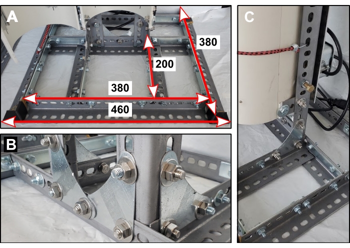
Figure 1: Reactor stand base. (A) Dimensions of base components in mm. (B) Orientation of metal corner gussets that secure the two vertical supports. (C) One of four short steel lengths connects the back half of the PVC pipe to the reactor stand. Please click here to view a larger version of this figure.

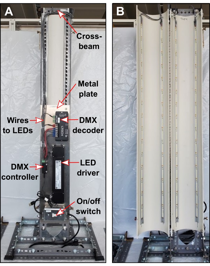
Figure 2: Electrical components. (A) Rearview of the PBR showing top cross beam and configuration of electrical components. (B) Front view of PBR after light installation. Please click here to view a larger version of this figure.

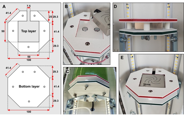
Figure 3: Bottle platform details. (A) Dimensions of top and bottom layer in mm. (B) Recessing bolt heads into both layers. (C) Braces connect the bottom layer directly to the rear half of the PVC pipe. (D) Five short pieces of rigid tubing fitted over narrow bolts hold the top and bottom layers apart. (E) When the bottle platform is complete, the surface should be flush. Please click here to view a larger version of this figure.

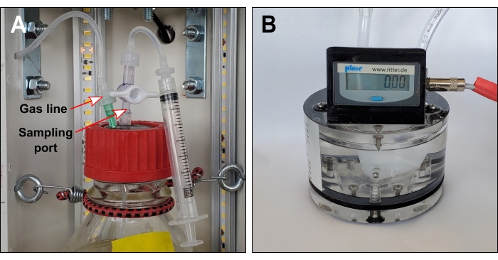
Figure 4: Gas line and optional sampling port. (A) Gas lines connect each bottle headspace to exterior gas sensors. If the sampling port is required, gas lines should include a one-way valve immediately downstream of the needle. (B) Volumetric gas sensor. The liquid packing level should touch the tracing screw. Please click here to view a larger version of this figure.

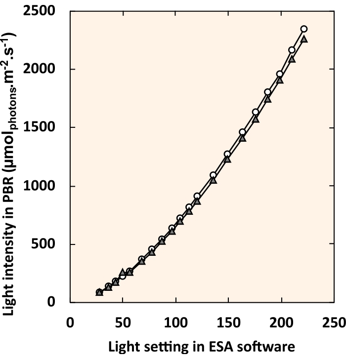
Figure 5: Standard curve relating LED control software settings to internal light intensity. White circles and gray triangles each represent an individual PBR. For each light setting, all four fixtures were set to an identical value. Please click here to view a larger version of this figure.

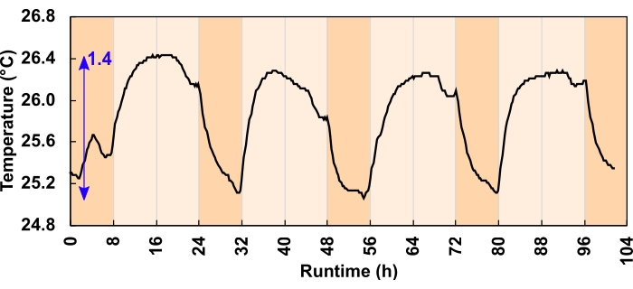
Figure 6: Culture temperature change for the 300 µmol_photons m^-2 s^-1 light regimes. During the 24 h, 16:8-h diurnal program, LEDs increased the daytime culture temperature. The blue arrow indicates the difference between the minimum and maximum temperature. A light program error caused the temperature dip before dusk; this was corrected before the experiment commenced. Please click here to view a larger version of this figure.

Figure 7: Oxygen production for three unique experimental conditions. Each reactor received a different combination of light intensity and initial biomass concentration (IBC); (A) 300 µmol_photons m^-2 s^-1 and IBC 0.03 g_AFDW L^-1, (B) 600 µmol_photons m^-2 s^-1 and IBC 0.13 g_AFDW L^-1, (C) 600 µmol_photons m^-2 s^-1 and IBC 0.40 g_AFDW L^-1. Top graphs display cumulative oxygen production (mL) and the gas flow rate (mL/h). Solid black lines, dashed blue lines, and dotted red lines are replicates. The runtime for each experiment was 104 h, which included four complete 16:8 h day-night cycles. Dark orange shading represents nighttime hours and light orange daytime hours. Note that in treatment B, oxygen production flatlines on day 4 for two of the three replicates. Please click here to view a larger version of this figure.

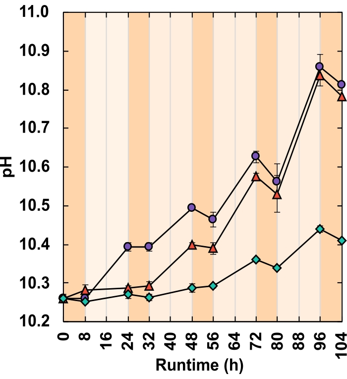
Figure 8: pH response. Each reactor received a different combination of light intensity and IBC;(green diamonds) 300 µmol_photons m^-2 s^-1 and IBC 0.03 g_AFDW L^-1, (red triangles) 600 µmol_photons m² s^-1 and IBC 0.13 g_AFDW L^-1, (purple circles) 600 µmol_photons m^-2 s^-1 and IBC 0.40 g_AFDW L^-1. Dark orange shading represents nighttime hours and light orange daytime hours. Error bars represent the standard error of the mean. Please click here to view a larger version of this figure.

Treatment	Light Intensity (µmol photons m-2 s-1)	IBC (gAFDW L-1)	Δ total biomass (gAFDW)	Δ pH	Total oxygen produced (mL)
A	300	0.031	0.289 (± 0.01)	0.15 (± 0.01)	316.2 (±11.4)
B	600	0.130	0.674 (± 0.02)	0.52 (± 0.27)	834.6*
C	600	0.400	0.675 (± 0.02)	0.55 (± 0.03)	902.2 (±50.5)
* Only one of the three replicates was successful

Table 1: Growth metric shift from hour 0 to 104. Brackets represent the standard error of the mean.

Treatment	Light Intensity (µmolphotons m-2 s-1)	IBC (gAFDW L-1)	Biomass growth measured (gAFDW)	Biomass growth predicted (gAFDW)	Underestimate (%)
A	300	0.031	0.289	0.288	0.5
A	300	0.031	0.311	0.270	13.1
A	300	0.031	0.268	0.247	7.9
B	600	0.13	0.708	0.705	0.4
C	600	0.4	0.718	0.796	-10.9
C	600	0.4	0.640	0.830	-29.7
C	600	0.4	0.668	0.659	1.3

Table 2: Growth estimates based on total measured oxygen. Only one replicate from the 300 µmol_photons m^-2 s^-1 and IBC = 0.13 g_AFDW L^-1 treatment ran to completion.

Supplementary Figure 1: Screenshot from LED control software. Each of the four light fixtures can be controlled independently by sliding the dimmer buttons or entering a numerical value into the text box. Please click here to download this File.

Supplementary Figure 2: Screenshot of the data acquisition software configuration window. Please click here to download this File.

Supplementary Figure 3: Screenshot of the data acquisition software logging window. Bright green rectangles indicate online gas sensors. Data is displayed in real-time. Please click here to download this File.

Supplementary Table 1: Example 24 h light regime. For a 16:8 h diurnal program, there are 48 sets of 30 min each. Asterisks indicate suggested sampling times. Please click here to download this Table.

Supplementary Table 2: High alkalinity high pH medium composition. Please click here to download this Table.

Supplementary Table 3: Trace element solution. Add to a final concentration of 1 mL/L to the base medium. Please click here to download this Table.

Discussion

Within this protocol, focus on the following steps increases the likelihood of generating reproducible, high-quality data. When constructing the reactor stand (step 1), the base must be sturdy with well-alligned vertical supports. Slotted steel has sharp edges, so the addition of safety caps is essential. Bottle platform surfaces need to be completely flat, the magnetic stirrer and bolt heads should both sit below the top layer surface (steps 3.2–3.6). According to the manufacturer's instruction, the gas sensor packing liquid should be filled to the "tracing screw for liquid level" for accurate oxygen measurements. This liquid level should be checked regularly as evaporation of the packing liquid can short-circuit the measurement cell. All three gas lines made in step 5.2 should be the same length; this enures that replicates have identical headspace volumes. Before commencing an experiment, it is advisable to test the programmed light regime by logging light intensity over a 24 h period (step 6.11). If increases in liquid temperature are of concern, this test should also include a sealed bottle with an internal temperature probe (step 6.11). When logging, do not exit the data acquisition software window; this will terminate logging. If taking culture samples, be careful not to release headspace gas by opening valves in the wrong sequence (steps 8.2-8.8). When reviewing experimental data be advised that the data acquisition software automatically generates a moving average of the flow rate. This inflates the value of the one or two flow rate readings generated overnight. Curate gas sensor logs manually to rectify this.

The most common setback with this method is the potential to short circuit the gas sensor if the liquid packing level declines. There are two ways this can occur. Firstly, evaporation can slowly reduce the liquid level. However, this is unlikely over a short-term (<7 day) experiment²⁹. Secondly, high respiration rates can pull oxygen into the solution and generate a headspace under-pressure. When light energy is unavailable, microalgae use aerobic respiration to supply the energy required for cellular maintenance and repair²⁸. Hence, in dense cultures during non-illuminated hours, oxygen consumption, and the resulting under-pressure, can be substantial. This sucks packing liquid from the gas sensors into the gas line. The distance the packing liquid travels is proportional to the amount of nighttime respiration. If the packing liquid enters the bottles, this generates an oil slick on the liquid surface.

If high nighttime respiration rates are expected, modifications to the protocol can be made. The simplest way to avoid under-pressure is to leave the bottle headspaces open overnight. This also has the advantage of easing DO levels by decreasing the partial headspace pressure of O₂. High DO concentrations are believed to be detrimental to growth as O₂ can impede the activity of Rubisco and may trigger oxidative stress^30,31. It is not uncommon for culture suspensions to reach 4x oversaturation even when in contact with the atmosphere^25,32. To open the headspace, disconnect the gas line from the needle spanning the rubber stopper. Nighttime hours can serve as a window to top up gas sensor packing liquid or manipulate continuous experiments with little impact on data collection. For example, one may alter the culture density, refresh nutrients, add an amendment, or introduce a pathogen. Bottles must be re-sealed, and the gas sensor line reconnected before lights turn back on. The oxygen measurements collected from experiments with closed versus open nighttime headspaces will differ.

When bottles remain sealed, nighttime oxygen consumption reduces the number of moles of O₂ in the headspace. This causes packing liquid to creep up the gas sensor line to maintain headspace pressure. When lights turn on, oxygen production resumes. Packing liquid must be pushed back into the gas sensor before flow rate readings commence. This lag is therefore proportional to the degree of nighttime respiration. In this way, when the headspace remains closed, O₂ readings represent net O₂ production (photosynthetic production - respiratory consumption). Conversely, when the headspace is open at night, atmospheric gas replaces what headspace O₂ is consumed, and no packing liquid enters the gas line. The result is that respiratory O₂ consumption is not accounted for in O₂ production data. This may reduce the accuracy of AFDW biomass growth estimates. However, it should not impact the utility of using daytime O₂ production as a metric to compare growth between treatments.

All laboratory PBRs are afflicted by the same limitation; artificial lights cannot replicate the solar spectrum. Microalgae use wavelengths of light between 400–700 nm for photosynthesis. This region is referred to as photosynthetically active radiation (PAR)³³. Sunlight and artificial light vary in their relative contribution of wavelengths within this range. This, alongside favorable temperatures and a constant light supply, means that laboratory growth data often cannot be reliably extrapolated to outdoor conditions. These PBRs can, however, address one of the limitations of laboratory PBR light supply. Sunlight intensity is highly variable throughout the day, with cloud cover generating transient fluctuations in incident PAR. The lighting control software and DMX lighting controller can provide light intensities from 0 to 2400 µmol_photons m^-2 s^-1 and beyond. Light regimes can be broken down into individual increments as short as 1 s. Tunable light intensity allows the user to mimic outdoor light patterns more closely than standard PBR setups. Here, simulated 30 min dawn and dusk intervals fade day and night cycles together (Supplementary Table 1).

Although AFDW density has become the standard measure of growth, this method can require substantial culture volumes, a 2–3-day processing period, and generates one data point at a time. Further, if conditions become unfavorable and cells die, AFDW density does not discriminate between actively photosynthesizing cells and those that are decomposing. Quantifying the rate of photosynthetic oxygen production serves as an alternative growth proxy. This PBR design can record oxygen production continuously with little user intervention while conserving culture volume. Data resolution could be improved by selecting a gas sensor with a lower measurement cell volume, e.g., 1 mL. Further, if cultures are well-mixed, users may decide to install a spectrophotometer for continuous optical density readings. If temperature control of the medium is desired, a recirculating chiller could be added. These PBRs are a valuable addition to a laboratory looking to expand its microalgal research capacity without heavy financial investment. They are particularly suitable for those working with high alkalinity, high pH species like Spirulina. These PBRs offer light regime flexibility and are valid for rapid, replicated, laboratory growth comparisons.

Materials

List of materials used in this article

Name	Company	Catalog Number	Comments
Aluminum channels Imperial: 0.90” x 39.37” Metric: 2.3 cm x 100 cm Quantity: 4	LED World	AC-AR1-1M	Required as a heat sink
Bungee cords, small Quantity: 5	-	-	To secure bottles
Computer - desktop/laptop Quantity: 1	-	-	-
Data Logger, HOBO U30 USB Weather Station Quantity: 1	HOBO, Hoskin	U30-NRC-VIA-10-S100-000	Records light sensor information
Digital interface module, Rigamo, 4-channel Quantity: 1	Ritter	N/A	This is to transmit gas sensor data to the computer
DMX decoder, 12~24 VDC, DMX-CV-4X5A Quantity: 1	LITECH, LED World	LT-840-6A	Transmit messages which alter the light pattern
DMX lighting controller, SUSHI-RB-RJ Quantity: 1	Arcolis, Nicolaudie America Inc.	SUSHI-RB-RJ DMX	Encodes the lighting program
Gas sensor packing liquid (Silox) Quantity: 1 L	Ritter	https://www.ritter.de/en/data-sheets/silox
Gas sensor, volumetric Quantity: 3	Ritter	MGC-1 V3.4 PMMA (https://www.ritter.de/downloads/mgc-milligascounter-en)	Measures oxygen production
Glass bottles, round 1 L with GL45 neck Quantity: 3	Corning, Capitol Scientific	1395-1L	Culture vessels
Hardware - end caps for slotted steel Quantity: 10	Paulin, Home Depot	142-612	To cover sharp edges of slotted steel
Hardware - eye hooks Quantity: 6	-	-	To secure bottles
Hardware - metal corner braces (large) Imperial: 4" x 4" Metric: 10 cm x 10 cm Quantity: 8	-	-	Larger brackets to construct metal stand
Hardware - metal corner braces (small) Imperial: 2 1/2" x 2 1/2" Metric: 6.4 cm x 6.4 cm Quantity: 6	-	-	Small brackets to connect bottle platforms to PVC pipe
Hardware - metal corner gussets Imperial: 3" x 3" Metric: 7.6 cm x 7.6 cm Quantity: 6	Paulin, Home Depot	142-616	Flat brackets to construct metal stand
Hardware - piano hinge Imperial: 36" Metric: 91 cm Quantity: 1	-	-	Connects two halves of PVC pipe
Hardware - rivets Quantity: 40	-	-	To attach piano hinge to PVC tubing
Hardware - set of bolts, nuts, washers Quantity: 60	-	-	Long thin bolts are required to secure bottle platforms around magentic stirrers
Hardware - set of bolts, nuts, washers Quantity: 30	-	-	Larger shorter bolts are required to build the metal stand
LED driver, constant voltage, 96W 24VDC UL Listed IP65 Driver Class 2 regulated power supply Quantity: 1	Magnitude Lighting, LED World	CVN96L24DC	Regulates power to the lights
LED lights, Cinco Bright LED Flex Strip Quantity: 4 m roll	EvenBright, LED World	FA128M57-4M-24V-X	Roll is trimmed into 4 x 1 m lengths and secured inside the PVC tube
Light meter, handheld with submersible sperical probe Quantity: 1	LI-COR	LA-250A	Calibrate the reactors light intensity
Light sensors Photosynthetic Light (PAR) Smart Sensor Quantity: 2	HOBO, Hoskin	S-LIA-M003	Only one is required however two would be good practice in case one malfunctioned
Magnetic stirrers (MIXdrive 1 XS) with external control units and power supply (MIXcontrol eco) Quantity: 3	2Mag, 2MAG USA	MF 40300	Stirrers sit sandwiched in bottle platforms
Metal plate Imperial: 24" x 8" Metric: 61 cm x 20.3 cm Quantity: 1	-	-	This is a surface on which to secure electronics, it is attached to the back of the reactor
Pipe, white PVC Imperial: 6" diameter x 42" high Metric: 15.2 cm x 106.7 cm Quantity: 1	-	-	Cut lengthwise in two halves, used to house lights and bottles
Plastic (HDPE) sheets Imperial: 4" x 4" x 1/4" Metric: 10 cm x 10 cm x 1 cm Quantity: 6	Inventables	30291-01	For bottle platforms which house magentic stirrers
Rubber stoppers - GL45 size Quantity: 3	Duran, VWR	76289-760	Seals culture vessels
Screw caps - with aperture and GL45 neck Quantity: 3	Corning, Capitol Scientific	1395-45HTSC	Generates seal of culture vessels
Slotted angle steel lengths Imperial: 1-1/2" X 48" x 0.074" Metric: 3.8 cm x 122 cm x 0.19 cm Quantity: 6	Paulin, Home Depot	142-202	Makes up the body of the metal stand
Slotted flat steel lenghts Imperial: 1-3/8" x 48" x 0.074" Metric: 3.5 cm x 122 cm x 0.19 cm Quantity: 3	Paulin, Home Depot	142-222	Makes up the body of the metal stand
Software - Easy Stand Alone (ESA)		https://www.dmxsoft.com/#apps	AKA LED control software
Software - Rigamo v3.1			AKA data acquisition software
Software - Storage Upgrade Tools (SUT)		https://store.dmxsoft.com//
Stir bar Imperial: 1" x 5/16" Metric: 2.5 cm x 0.8 cm Quantity: 3	Fisherbrand	14-513-59	Stirs culture
Switch box Quantity: 1	-	-	Turns power on/off to reactor
Syringe, 10 mL Quantity: Multiple	-	-	Optional if you wish to extract culture
Tube adaptor fittings, plastic - Stopcock 1-way Quantity: 6	Masterflex, Cole Palmer	RK-12023-33	Close/open culture vessel line
Tube adaptor fittings, plastic - variety of male and female luer lock fittings Imperial: to fit 1/16" and 1/8" ID tubing Metric: to fit 1.59 mm and 3.18 mm tubing Quantity: Multiple packets	Masterflex, Cole Palmer	RK-30800-16; RK-30800-18; RK-45518-26; RK-45501-00; RK-45501-04	Many different combinations can achieve the same end result, best to order a variety of fittings
Tube adaptor fittings, plastic - variety of straight connectors Imperial: to fit 1/16" and 1/8" ID tubing Metric: to fit 1.59 mm and 3.18 mm tubing Quantity: Multiple packets	Masterflex, Cole Palmer	RK-40616-04	Many different combinations can achieve the same end result, best to order a variety of fittings
Tubing, flexible, transparent Imperial: ID=1/16", OD=1/8" Metric: ID = 1.59 mm, 0D = 3.18 mm Quantity: 4 m	Masterflex, Cole Palmer	RK-06422-02	Line from culture vessel to gas sensor
Tubing, flexible, transparent Imperial: ID=1/8", OD=1/4" Metric: ID = 3.18 mm, 0D = 6.35 mm Quantity: 2 m	Masterflex, Cole Palmer	RK-06422-05	Gas sensor standard tubing size
Tubing, rigid, transparent Imperial: ID=1/16", OD=1/8" Metric: ID = 1.59 mm, 0D = 3.18 mm Quantiy: 1 m	Masterflex, Cole Palmer	RK-06605-27	Spans rubber stopper allowing gas to exit
Tubing, rigid, transparent Imperial: ID=1/8", OD=1/4" Metric: ID = 3.18 mm, 0D = 6.35 mm Quantity: 1 m	Masterflex, Cole Palmer	RK-06605-30	Spans rubber stopper allowing gas to exit
Zip ties, small Quantity: 1 packet			Secure tube fittings

References

- Benemann, J. R. Opportunities and challenges in algae biofuels production. A position paper in line with Algae World. , (2008).
- Laurens, L. M. L. State of technology review - algae bioenergy. An IEA bioenergy inter-task strategic project. IEA Bioenergy. , (2017).
- Robertson, D. E., et al. A new dawn for industrial photosynthesis. Photosynthesis Research. 107, 269-277 (2011).
- Troschl, C., Meixner, K., Drosg, B. Cyanobacterial PHA production-review of recent advances and a summary of three years' working experience running a pilot plant. Bioengineering. 4 (2), (2017).
- Rizwan, M., Mujtaba, G., Memon, S. A., Lee, K., Rashid, N. Exploring the potential of microalgae for new biotechnology applications and beyond: a review. Renewable and Sustainable Energy Reviews. 92, 394-404 (2018).
- Niesa, F., et al. Characterization of Phormidium lacuna strains from the North Sea and the Mediterranean Sea for biotechnological applications. Process Biochemistry. 59, 194-206 (2017).
- Laurens, L. M. L., Chen-Glasser, M., McMillan, J. D. A perspective on renewable bioenergy from photosynthetic algae as feedstock for biofuels and bioproducts. Algal Research. 24, 261-264 (2017).
- Barreiro-Vescovo, S., Barbera, E., Bertucco, A., Sforza, E. Integration of microalgae cultivation in a biogas production process from organic municipal solid waste: From laboratory to pilot scale. ChemEngineering. 4 (2), 26(2020).
- Zurano, A. S., et al. Year-long assessment of a pilot-scale thin-layer reactor for microalgae wastewater treatment. Variation in the microalgae-bacteria consortium and the impact of environmental conditions. Algal Research. 50, (2020).
- Deprá, M. C., Severo, I. A., Dias, R. R., Zepka, L. Q., Jacob-Lopes, E. Photobioreactor design for microalgae culture. Microalgae. , Elsevier. 35-61 (2021).
- Osburn, F. S., Wagner, N. D., Scott, J. T. Biological stoichiometry and growth dynamics of a diazotrophic cyanobacteria in nitrogen sufficient and deficient conditions. Harmful Algae. 103, (2021).
- Eustance, E., Badvipour, S., Wray, J. T., Sommerfeld, M. R. Biomass productivity of two Scenedesmus strains cultivated semi-continuously in outdoor raceway ponds and flat-panel photobioreactors. Journal of Applied Phycology. 28 (3), 1471-1483 (2016).
- Qiang, H., Richmond, A., Zarmi, Y. Combined effects of light intensity, light-path and culture density on output rate of spirulina platensis (cyanobacteria). European Journal of Phycology. 33 (2), 165-171 (1998).
- Ooms, M. D., Dinh, C. T., Sargent, E. H., Sinton, D. Photon management for augmented photosynthesis. Nature Communications. 7, 1-13 (2016).
- Moheimani, N. R., Borowitzka, M. A., Isdepsky, A., Sing, S. F. Standard methods for measuring growth of algae and their composition. Algae for biofuels and energy. , Springer. Dordrecht. 265-284 (2013).
- Griffiths, M. J., Garcin, C., van Hille, R. P., Harrison, S. T. L. Interference by pigment in the estimation of microalgal biomass concentration by optical density. Journal of Microbiological Methods. 85 (2), 119-123 (2011).
- Schumann, R., Häubner, N., Klausch, S., Karsten, U. Chlorophyll extraction methods for the quantification of green microalgae colonizing building facades. International Biodeterioration and Biodegradation. 55 (3), 213-222 (2005).
- Pinckney, J. L., Richardson, T. L., Millie, D. F., Paerl, H. W. Application of photopigment biomarkers for quantifying microalgal community composition and in situ growth rates. Organic Geochemistry. 32 (4), 585-595 (2001).
- Van Wychen, S., Laurens, L. M. L. Determination of total solids and ash in algal biomass: laboratory analytical procedure (LAP). National Renewable Energy Laboratory. , Golden, CO. (2015).
- Davis, R., Laurens, L. Algal biomass production via open pond algae farm cultivation: 2019 state of technology and future research. National Renewable Energy Laboratory. , Golden, CO. (2020).
- Borovkov, A. B., Gudvilovich, I. N., Avsiyan, A. L. Scale-up of Dunaliella salina cultivation: from strain selection to open ponds. Journal of Applied Phycology. 32 (3), 1545-1558 (2020).
- Davies, F. K., et al. Microbiota associated with the large-scale outdoor cultivation of the cyanobacterium Synechococcus sp. PCC 7002. Algal Research. 58, (2021).
- Ataeian, M., et al. Direct capture and conversion of CO2 from air by growing a cyanobacterial consortium at pH up to 11.2. Biotechnology and Bioengineering. 116 (7), 1604-1611 (2019).
- Fu, F., et al. Sustained photosynthesis and oxygen generation of microalgae-embedded silk fibroin hydrogels. ACS Biomaterials Science & Engineering. , (2021).
- Rearte, T. A., et al. Photosynthetic performance of Chlorella vulgaris R117 mass culture is moderated by diurnal oxygen gradients in an outdoor thin layer cascade. Algal Research. 54, (2021).
- Poughon, L., et al. Limnospira indica PCC8005 growth in photobioreactor: model and simulation of the ISS and ground experiments. Life Sciences in Space Research. 25, 53-65 (2020).
- Yen, U. C., Huang, T. C., Yen, T. C. Observation of the circadian photosynthetic rhythm in cyanobacteria with a dissolved-oxygen meter. Plant Science. 166 (4), 949-952 (2004).
- Vermaas, W. F. Photosynthesis and respiration in cyanobacteria. eLS. , (2001).
- Ritter, MilliGascounter Type MGC-1 Operation Instructions V 3.4. , (2017).
- Sousa, C., De Winter, L., Janssen, M., Vermuë, M. H., Wijffels, R. H. Growth of the microalgae Neochloris oleoabundans at high partial oxygen pressures and sub-saturating light intensity. Bioresource Technology. 104, 565-570 (2012).
- Latifi, A., Ruiz, M., Zhang, C. C. Oxidative stress in cyanobacteria. FEMS microbiology reviews. 33 (2), 258-278 (2009).
- Morillas-España, A., Lafarga, T., Gómez-Serrano, C., Acién-Fernández, F. G., González-López, C. V. Year-long production of Scenedesmus almeriensis in pilot-scale raceway and thin-layer cascade photobioreactors. Algal Research. 51, (2020).
- Melis, A. Solar energy conversion efficiencies in photosynthesis: minimizing the chlorophyll antennae to maximize efficiency. Plant Science. 177 (4), 272-280 (2009).
Reprints and Permissions