Reconstituting and Characterizing Actin-Microtubule Composites with Tunable Motor-Driven Dynamics and Mechanics

Summary

This paper presents protocols for engineering and characterizing tunable three-dimensional composite networks of co-entangled actin filaments and microtubules. Composites undergo active restructuring and ballistic motion, driven by myosin II and kinesin motors, and are tuned by the relative concentrations of actin, microtubules, motor proteins, and passive crosslinkers.

Abstract

The composite cytoskeleton, comprising interacting networks of semiflexible actin filaments and rigid microtubules, restructures and generates forces using motor proteins such as myosin II and kinesin to drive key processes such as migration, cytokinesis, adhesion, and mechanosensing. While actin-microtubule interactions are key to the cytoskeleton's versatility and adaptability, an understanding of their interplay with myosin and kinesin activity is still nascent. This work describes how to engineer tunable three-dimensional composite networks of co-entangled actin filaments and microtubules that undergo active restructuring and ballistic motion, driven by myosin II and kinesin motors, and are tuned by the relative concentrations of actin, microtubules, motor proteins, and passive crosslinkers. Protocols for fluorescence labeling of the microtubules and actin filaments to most effectively visualize composite restructuring and motion using multi-spectral confocal imaging are also detailed. Finally, the results of data analysis methods that can be used to quantitatively characterize non-equilibrium structure, dynamics, and mechanics are presented. Recreating and investigating this tunable biomimetic platform provides valuable insight into how coupled motor activity, composite mechanics, and filament dynamics can lead to myriad cellular processes from mitosis to polarization to mechano-sensation.

Introduction

The cytoskeleton is a dynamic composite network of interacting biopolymers that provides structural and mechanical support to cells. Associated molecular motors and binding proteins restructure and adapt the cytoskeleton to allow cells to grow, change shape, stiffen, move, and even self-heal, enabling myriad cellular processes ranging from migration and division to mechanosensing^1,2. Beyond its significance in cellular biophysics, the cytoskeleton is also a quintessential example of active matter with potential materials applications ranging from wound healing and drug delivery to filtration and soft robotics^{1,3,4,5,6,7,8,9}.

The two key characteristics that endow the cytoskeleton with its unique structural and mechanical diversity and multifunctionality are: 1) its composite nature, comprising multiple interacting protein filaments, such as semiflexible actin filaments and rigid microtubules, as well as their associated binding and crosslinking proteins^3,5,10; and 2) its ability to continuously restructure, move, coarsen, and perform work via energy-consuming motors, such as myosins and kinesins, pushing and pulling on the filamentous proteins^1,7,11,12,13. While this elegant complexity enables the cytoskeleton to mediate processes as diverse as cell motility, cytokinesis, and wound-healing^3,6,7,11, it hampers the ability of researchers to reproduce the signature in vivo characteristics of the cytoskeleton in reconstituted in vitro systems.

Current frontier reconstitution efforts focus on composites of entangled and crosslinked actin filaments and microtubules^{3,10,14,15,16,17}, force-generating actomyosin networks^{2,8,18,19,20,21}, and active nematics driven by kinesin-microtubule interactions^{22,23,24,25,26}. Steady-state actin-microtubule composites have been shown to display emergent mechanical properties^15,16,27, such as enhanced filament mobility and increased stiffness compared to single-component systems²⁷. Studies on in vitro actomyosin systems have reported a wide range of structural and dynamical properties that depend on the concentrations of actin, myosin, and crosslinkers^28,29,30,31. For example, with sufficient crosslinking, actomyosin networks undergo large-scale contraction and coarsening^{2,28,30,32,33,34,35,36}, whereas without crosslinkers, networks display rapid, destabilizing flow and rupturing^19,29. Reconstituted microtubule-based active nematics that use clusters of kinesin motors to crosslink and pull on microtubule bundles have been reported to exhibit long lasting turbulent flows, extension, buckling, fracturing, and healing^{12,22,23,24,25,37,38,39,40,41,42,43,44,45,46,47}.

More recently, actin-microtubule composites driven by myosin II mini-filaments have been shown to lead to more ordered contraction and network integrity compared to the disordered flow and network rupturing that actomyosin networks without crosslinkers exhibit^17,26,48. Moreover, the combination of composite robustness and force-generation is optimized when actin and microtubules are present at comparable concentrations. Key emergent features in this region of formulation space include enhanced mechanical strength²⁶, coordinated motion of actin and microtubules²⁶, steady sustained contraction, and mesoscale restructuring¹⁷.

Here, protocols are described to engineer and tune co-entangled and crosslinked composites of microtubules and actin filaments that are pushed out of equilibrium by myosin II mini-filaments and kinesin clusters acting on actin filaments and microtubules, respectively (Figure 1). The dynamics, structure, and mechanics of this class of composites can be tuned by the relative concentrations of the filaments, motors, and crosslinkers to exhibit a rich phase space of advective and turbulent flow, isotropic contraction, acceleration, deceleration, de-mixing, stiffening, relaxation, and rupturing. The focus of this work is on preparing and tuning this class of active cytoskeletal composites. However, to aid researchers in benchmarking and characterizing the described active composites, effective imaging methods using multi-spectral confocal microscopy are also detailed. Finally, results of key computational analysis methods that can be used to measure the dynamics, structure, and mechanics of the composites are presented. Researchers are encouraged to adopt these methods-which include differential dynamic microscopy (DDM), spatial image autocorrelation (SIA), and particle image velocimetry (PIV)-as they have been optimized to characterize the complex dynamics and structural diversity of the composites^17,26,49.

The steps described below focus on preparing the composites and imaging them using confocal microscopy. Protocols describing post-acquisition data analysis and optical tweezers measurements can be found in previous works ^17,26,48,50, and provided upon request. All materials are listed in the Table of Materials provided.

Protocol

1. Prepare silanized coverslips and microscope slides to prevent adsorption of proteins to chamber surfaces

NOTE: This is a 2-day process. Silanized slides may be prepared up to 1 month in advance of use.

1. Place no. 1 coverslips (24 mm x 24 mm) and microscope slides (1 in x 3 in) in a designated rack that will fit in the plasma cleaner. Place rack in plasma cleaner and run for 20 min.
2. Transfer coverslips and slides to a new rack designated only for use with silane and place rack in glass container to clean the glasses as described below.
   1. Immerse coverslips and slides in 100% acetone for 1 h. Immerse coverslips and slides in 100% ethanol for 10 min.
   2. Immerse coverslips and slides in deionized water (DI) for 5 min. Repeat the cleaning steps two more times.
   3. Immerse coverslips and slides in freshly prepared 0.1 M KOH for 15 min. Immerse coverslips and slides in fresh DI for 5 min. Repeat this step two more times.
3. Air dry coverslips and slides for 10 min. Treat cleaned coverslips and slides with silane to produce hydrophobic surfaces as described below.
   NOTE: Complete the following steps in a fume hood.
   1. Immerse dried coverslips and slides in 2% silane (dissolved in toluene) for 5 min. Use a funnel to pour silane back into its designated bottle to reuse up to five times.
   2. Immerse coverslips and slides in 100% ethanol for 5 min. Replace ethanol with fresh ethanol. Immerse coverslips and slides for 5 min.
   3. Immerse coverslips and slides in fresh DI for 5 min. Repeat the ethanol and DI wash step two more times using fresh ethanol and DI each time. Air dry coverslips and slides for 10 min.

2. Preparing active actin-microtubule composite driven by myosin mini-filaments

1. Remove inactive myosin via actin filament binding and perform pull-down via ultracentrifugation as described below.
   1. Polymerize actin into filaments. Using a precision micropipette and sterile pipet tips, combine in a microcentrifuge tube: 1.87 µL of DI, 1.3 µL of 10x G-buffer, 1.3 µL of 10x F-buffer, 1.63 µL of 4 M KCl, 4.53 µL of actin (47.6 µM), and 1.08 µL of 100 µM phalloidin.
      NOTE: To ensure sufficient polymerization, the actin concentration and actin:phalloidin molar ratio should be 18.4 µM and 2:1, respectively.
   2. Gently pipet the solution up and down to mix and then set on ice in the dark for ≥1 h. Cool ultracentrifuge to 4 °C. Remove myosin aliquot from -80 °C and put on ice.
      NOTE: Complete step 2.2 at this point while actin is polymerizing.
   3. After ≥1 h of actin polymerization, add 1.3 µL of 10 mM ATP and 2 µL of 19 µM myosin to the polymerized actin.
      NOTE: The actin:myosin molar ratio should be >5 to ensure sufficient removal of inactive myosin motors (i.e., dead heads).
   4. Gently pipet the solution up and down to mix. Transfer into an ultracentrifuge grade tube.
      ​Centrifuge at 4 °C and 121,968 x g for 30 min.
2. Prepare co-entangled composite network of actin filaments and microtubules as described below.
   NOTE: Begin 30 min before myosin spin-down (step 2.1.4).
   1. Set a heat block to 37 °C. Use a precision micropipette and sterile pipet tips to add the following to a microcentrifuge tube: 13.9 µL of PEM, 3 µL of 1% Tween20, 1.55 µL of 47.6 µM actin, 0.36 µL of 34.8 µM R-actin, 0.3 µL of 250 mM ATP, 0.87 µL of 100 µM phalloidin, 1.91 µL of 5-488-tubulin, 0.3 µL of 100 mM GTP, and 0.75 µL of 200 µM Taxol, to a total volume of 23 µL.
      NOTE: The concentrations of actin and tubulin listed are for a composite with 2.9 µM actin and 2.9 µM tubulin. Total protein concentration is c = c_A + c_T = 5.8 μM and molar actin fraction is c_A/(c_A + c_T) = Φ_A = 0.5. See step 2.5 to adjust these values.
   2. Gently pipet the solution up and down to mix and place on a 37 °C heat block protected from light for 1 h.
3. Prepare sample chambers for confocal imaging experiments as described below.
   NOTE: Complete steps 2.1.4 and 2.2.2 during waiting periods.
   1. Place two silanized slides side-by-side on a hot plate (turned off), lay two strips of thermoplastic sealing film across the slides ~3 mm apart, and place two silanized coverslips over the thermoplastic sealing film to form a sample chamber.
   2. Turn the hot plate on low setting until coverslips firmly bind to slides with melted thermoplastic sealing film (~1-2 min). Press down with even pressure to ensure bonding while maintaining ~100 µm spacing between the two surfaces.
   3. Remove chambers and turn off hot plate. Label chambers with (+) and (-). The (+) chamber will be for the active sample (with myosin) and the (-) chamber will be the control (no myosin). Ensure each chamber can accommodate ≤10 µL of fluid.
4. Prepare samples to image as described below.
   NOTE: It is important to complete this step immediately after steps 2.1 and 2.2 are completed.
   1. Carefully remove the myosin-actin sample from the ultracentrifuge (step 2.1.4) and immediately pipet up the top 7.5 µL of the supernatant and transfer to a new microcentrifuge tube.
   2. Remove the actin-microtubule sample from the heat block and gently mix in 1.5 µL of 10x D-Glucose, 1.5 µL of 10x GOC, and 1.5 µL of 1 mM blebbistatin. Divide the solution into two 13.7 µL aliquots and label as (+) and (-).
   3. Mix in 1.28 µL of the supernatant from step 2.4.1 to (+) aliquot. Mix in 1.28 µL of DI to the (-) aliquot. Slowly flow each solution into the corresponding chamber (step 2.3) via capillary action. Be careful not to introduce air bubbles into the channel.
   4. Seal the two open ends of each channel with fast-drying epoxy or UV glue. Ensure the adhesive is completely dry before placing on the microscope. Image immediately as described in step 3.
      NOTE: UV glue is advantageous because it cures nearly instantly upon UV exposure. However, because blebbistatin is UV sensitive, it is important to only locally illuminate the glue (at the edges of the sample chamber) using a small UV wand to avoid deactivating the blebbistatin.
5. Optional: vary the protein concentrations to tune the dynamics and structure of the composites.
   NOTE: The following steps are suggested alterations to the steps above to vary the concentrations of actin, microtubules, and myosin if desired.
   1. Follow the steps described above except for the following modifications in steps 2.2.1 and 2.4.3.
   2. To vary the concentrations of actin and microtubules, thereby adjusting c and Φ_A, increase or decrease the volume of actin, R-actin, and 5-488-tubulin used in step 2.2.1, as desired²⁶. When varying the actin concentration, adjust R-actin and phalloidin molar concentrations proportionally to maintain the same molar ratios with actin. Adjust the volume of PEM such that the final volume of the mixture remains 23 µL. All other component volumes and concentrations remain the same.
   3. To vary the myosin concentration, adjust the volume of myosin added to the (+) aliquot in step 2.4.3 as desired. Adjust the DI volume added to the (-) aliquot accordingly. Adjust the PEM volume in Step 2.2.1 to account for the increase or decrease in myosin (+) and DI (-) volume, ensuring the final volume of each sample ((+) and (-)) is 14.98 μL.

3. Imaging and characterization of active composites using confocal microscopy

1. To image actomyosin-microtubule composites prepared in step 2, use a laser scanning confocal microscope (LSCM), or similar microscope, with a 60x 1.4 NA oil-immersion objective. To simultaneously visualize actin filaments and microtubules in separate fluorescence channels, use a 561 nm laser with 565/591 nm excitation/emission filters and a 488 nm laser with 488/525 nm excitation/emission filters.
2. Place the sample chamber on the microscope such that the control channel is positioned directly over the objective. Make sure there is an oil interface between the objective and the coverslip.
3. Use the stage controls to bring the control composite into focus, then find both surfaces of the sample chamber. Move the z position to the center of the sample chamber. Check for the presence of clear filamentous networks as shown in Figure 2.
4. Still visualizing the control chamber, adjust the intensity of each laser to allow for simultaneous visualization of actin filaments and microtubules. Maintain the lowest laser intensity possible to prevent photobleaching (more prevalent in the actin channel) and bleed through (typically from the microtubules into the actin channel).
5. To characterize the inactive control sample, collect three time-series (videos) of 256 x 256 square-pixel (213 µm x 213 µm) images at 2.65 fps for a total of ≥1000 frames. Collect each time-series in a different region of the sample chamber separated by ≥500 µm. Ensure that there is minimal detectable motion and no flow or restructuring.
6. Shutter off the 488 nm laser and use the stage controls to move to the (+) chamber.
7. Using the 568 nm laser, visualize the microtubules in the (+) channel to ensure proper network formation (Figure 2) and identify the axial center of the sample chamber (which may be different to the center z-position of the control chamber).
8. Turn on the 488 nm laser and repeat step 3.5 above with the following modifications. Collect time-series for up to 45 min, stopping acquisition when the sample either moves out of the field of view, ruptures, or photobleaches. Record 5-10 time-series and keep track of the time at which each time-series begins relative to the start of the first time-series.
9. Analyze data using DDM, SIA, and PIV as described in Figure 3, Figure 4, Figure 5, and previously^17,48,50,51.
   ​NOTE: The 488 nm laser locally activates myosin ATPase activity by de-activating blebbistatin, so it should only be turned on at the start of data acquisition such that t = 0 is at the start of the time-series. These acquisition parameters are optimized for differential dynamic microscopy (DDM) analysis as done previously²⁶.

4. Preparation of active actin-microtubule composites driven by kinesin motors

NOTE: The following steps create actin-microtubule composites that are driven out-of-equilibrium by kinesin motors or a combination of kinesin and myosin⁵⁰.

1. Prepare kinesin and myosin motors as described below.
   1. If incorporating myosin, follow step 2.1.
   2. To form kinesin motor clusters that bind and exert forces between pairs of microtubules, use a micropipette and sterile pipet tips to add the following to a sterile 1.5 mL microcentrifuge tube:1.16 µL PEM, 2.74 µL 8.87 µM kinesin dimers, 7.29 µL 83.3 µM NeutrAvidin, 0.81 µL 2mM DTT . Mix gently by pipetting the solution up and down and incubate protected from light (use a black microcentrifuge tube or wrap in foil) for 30 min at 4 °C.
      NOTE: The molar ratio of kinesin dimers to NA is 1:25.
2. Follow step 2.3 to prepare sample chambers and make three chambers instead of two. Carry out this step during kinesin incubation (step 4.1.2) and myosin ultracentrifugation (step 4.1.1).
3. Prepare co-entangled composite network of actin filaments and microtubules.
   1. Set heat block to 37 °C. Use a micropipette and sterile pipet tips to add the following to a sterile 1.5 mL microcentrifuge tube: 3.21 µL PEM, 4.5 µL of 1% Tween20, 2.18 µL of 47.6 µM actin, 3.46 µL of 5-R-tubulin, 4.5 µL of 100 mM ATP, 4.5 µL of 10 mM GTP, 1.13 µL of 200 µM Taxol, and 1.57 µL of 20 µM 488-phalloidin. Ensure the total volume is 25 µL.
   2. Gently pipet the solution up and down to mix and place on the 37 °C heat block protected from light for 1 h. Remove the tube from the heat block and use a micropipette to gently mix in 0.84 µL of 100 μM phalloidin. Incubate for 5-10 min at room temperature, protected from light.
      NOTE: Adding phalloidin at this step, rather than in step 4.3.1, improves the fluorescence labeling of actin filaments, as 488-phalloidin does not have to compete with unlabeled phalloidin for actin binding sites.
4. Prepare active composites for confocal imaging.
   1. Add 1.13 µL of 200 μM blebbistatin, 1.35 µL of 10x Glu, and 1.35 µL of 10x GOC to the solution from step 4.3.2 and mix gently by pipetting up and down. Divide the solution into three 10 µL aliquots and label as (K), (K+M), and (-).
   2. Mix in 2.54 µL of myosin from step 2.1.4 to the (K+M) aliquot. Mix in 2.54 µL PEM to (K) and (-) aliquots.
   3. Use a micropipette and sterile pipet tips to add 2.5 µL of kinesin clusters from step 4.1.2 to (K) and (K+M) aliquots. Pipet up and down to mix. Mix in 2.5 µL PEM to (-) using the same technique.
      NOTE: The concentrations of actin and tubulin listed are for a composite with 2.32 µM actin and 3.48 µM tubulin. Total protein concentration is c = c_A + c_T = 5.8 μM and molar actin fraction is c_A/(c_A + c_T) = Φ_A = 0.4. Kinesin and myosin concentrations are 0.35 µM and 0.47 µM, respectively. See step 2.5 for general guidelines to adjust c_A, c_T, c, and Φ_A.
   4. Using a micropipette, slowly flow each solution into the corresponding channel of the prepared sample chambers (step 4.2) via capillary action. Push down very slowly and gently on the pipet so as to not introduce air bubbles into the channel.
   5. Seal the two open ends of each channel with fast-drying epoxy or UV-curable glue. Ensure the adhesive is completely dry before placing on the microscope.
      NOTE: It is important that this step is done quickly to minimize the time that the kinesin is acting without being monitored. For this reason, epoxy that cures in 1 min (rather than 5 or 10 min) is recommended. UV-curable glue is advantageous in this regard because it cures nearly instantly upon UV exposure. 
5. Image prepared samples immediately, following step 3, except for the following important modifications. Because kinesin is not controlled by light-activation, it starts to work immediately after step 4.4.3, so mark this time as t = 0. To image the composite as close to the initial inactive state (t = 0) as possible, image the (K) and (K+M) channels first and note the time elapsed between step 4.4.3 and the beginning of data acquisition (step 3.8). In practice, this elapsed time is ~5 min.

5. Incorporating passive crosslinkers into active composites

NOTE: These steps describe how to use biotinylated actin and tubulin subunits and NeutrAvidin (NA) to passively crosslink actin to actin (A-A) or microtubules to microtubules (M-M) in the active composites described in step 4.

1. Prepare A-A or M-M crosslinker complexes with biotinylated proteins (biotin-actin or biotin-tubulin), NA, and biotin at a ratio of 2:2:1 biotin-actin/tubulin:biotin:NA. Start this process before Step 4 .
   1. For A-A crosslinkers, use a micropipette and sterile pipet tips to add 2 µL of 11.6 µM biotin-actin, 1.39 µL of 8.33 µM NA, 2.27 µL of 1.02 µM biotin, and 4.34 µL of PEM to a microcentrifuge tube. Mix gently by pipetting up and down.
   2. For M-M crosslinkers, use a micropipette and sterile pipet tips to add 1.86 µL of 4.55 µM biotin-tubulin, 1.11 µL of 8.33 µM NA, 1.82 µL of 1.02 µM biotin, and 5.21 µL of PEM to a microcentrifuge tube. Mix gently by pipetting up and down.
   3. Wrap the tube(s) from step 5.1.1 and/or 5.1.2 in thermoplastic sealing film to create a water-tight seal. Place in a flotation raft in a temperature-controlled sonicator bath set to 4 °C.
   4. Sonicate for 90 min at 4 °C. In practice it is best to put the sonicator in a cold room and add ice packs to the sonication bath to maintain low temperature.
2. To incorporate crosslinker complexes into samples for imaging, follow step 4.3, modifying step 4.3.1 as described below for A-A crosslinking (step 5.2.1) or M-M crosslinking (step 5.2.2).
   1. For A-A crosslinking, combine the following in a microcentrifuge tube: 1.94 µL of PEM, 4.50 µL of 1% Tween20, 2.18 µL of 47.6 µM actin, 3.46 µL of 45.5 µM 5-R-tubulin, 1.13 µL of A-A crosslinkers (step 5.1.1), 4.50 µL of 100 mM ATP, 4.50 µL of 10 mM GTP, 1.13 µL of 200 µM Taxol, and 1.57 µL of 20 µM 488-phalloidin. Ensure the total volume is 25 µL.
   2. For M-M crosslinking, combine the following in a microcentrifuge tube: 1.97 µL of PEM, 4.50 µL of 1% Tween20, 2.18 µL of 47.6 µM actin, 3.76 µL of 45.5 µM 5-R-tubulin, 1.13 µL of 1:4 dilution of M-M crosslinkers (step 5.1.2), 4.50 µL of 100 mM ATP, 4.50 µL of 10 mM GTP, 1.13 µL of 200 µM Taxol, and 1.57 µL of 20 µM 488-phalloidin. Ensure the total volume is 25 µL.
3. Follow steps 4.3.2-4.5 with the specific concentrations for a crosslinker:actin molar ratio of R_A = 0.02 and crosslinker:tubulin molar ratio of R_T = 0.005. These R_A and R_T values result in similar lengths between crosslinkers along actin filaments and microtubules (d_A  60 nm and d_MT  67 nm), estimated using d_A = I_monomer/2R_A, where I_monomer is the length of an actin monomer, and d_MT = I_ring/26R_T, where I_ring is the length of a ring of 13 tubulins^15,17.

Results

To determine successful preparation of active composites (Figure 1), and to characterize their dynamics and structure, a laser scanning fluorescence microscope with at least two fluorescence channels is used to visualize the actin filaments and microtubules simultaneously (Figure 2 and Figure 6). All actin filaments and microtubules in the composites are sparsely labeled, rather than doping in tracer bright filaments, as is often done in in vitro studies. This method ensures that the measured dynamics and structure are representative of the composite itself rather than the tracers which are formed under different conditions than the composites. For this reason, individual actin filaments and microtubules cannot typically be resolved, rather images portray mesoscale network structure (Figure 2 and Figure 6).

This labeling approach was optimized for spatial image autocorrelation (SIA) and differential dynamic microscopy (DDM) analyses that examine the dynamics and structure in reciprocal Fourier space (Figure 4, Figure 5, and Figure 8)^52,53,54,55. Particle-image velocimetry (PIV) can also be used to depict and characterize dynamics and flow fields (Figure 3 and Figure 7), but it requires pixel-binning (lower spatial resolution) and larger lag-time increments (lower temporal resolution) than SIA and DDM to eliminate erroneous vectors that arise from noise in the dense, low-signal images. Nevertheless, PIV is recommended for qualitative examination of flow fields and corroboration of DDM results (Figure 4 and Figure 8)^26,50.

Sample characterization of the described networks using these analyses (i.e., DDM, SIA, PIV) is provided to aid researchers in adopting similar analyses to benchmark and characterize their samples. However, detailed descriptions of these techniques are outside the scope of this work. For detailed descriptions of how to perform DDM on these and other similar systems, including user-friendly Python code, refer to previous works^17,26,49,50 and the references there within. For details regarding how to perform SIA and PIV on the systems described here, the reader is directed to previous works^17,50.

Several controls, described below, should be done to ensure that the composites are functioning as expected. A composite without myosin or kinesin should appear essentially static with minimal thermal fluctuations or drift. Actin filaments and microtubules should appear co-entangled and homogeneously distributed, with minimal bundling, aggregation, or phase separation of actin and microtubules throughout a field of view of ~200 µm x 200 µm (Figure 2, far left)¹⁷. One should expect a similar result for composites that contain myosin but are not exposed to 488 nm light (to deactivate the blebbistatin).

Upon incorporation of myosin and exposure to 488 nm light, the composites undergo contraction that is largely isotropic and similar for actin and microtubules, as seen in microscope images taken before and after myosin activity (Figure 2), as well as corresponding PIV flow fields for varying times during activity (Figure 3). To determine if the motion is ballistic, diffusive, subdiffusive, etc., the characteristic decorrelation time τ(q) determined from DDM is evaluated as a function of wave vector (i.e., reciprocal space). See as described in detail previously^17,26,49. Figure 4 also demonstrates how to use DDM to characterize these composites. Power-law scaling τ(q)~1/vq^β, with β = 1, indicates ballistic motion with speed v. For reference, β = 2 represents diffusive dynamics with v being the diffusion coefficient. All active composites exhibit ballistic scaling (Figure 4A) with speeds that are tuned by the concentrations of actin and myosin (Figure 4B), and that can vary in time during activity, either accelerating or decelerating (Figure 4C,D).

Network restructuring and clustering, visible in Figure 2 and more evident for higher actin and myosin concentrations, can be characterized using SIA, as depicted in Figure 5, and described previously^17,48,50. Briefly, a correlation length ξ, which is a measure of the characteristic size of features in an image, can be determined by fitting each spatial intensity autocorrelation curve g(r) to an exponential function of distance r between pixels. Larger g(r) peaks that persist for longer distances indicate larger structural features (i.e., bundling, clustering of the individual filaments). As shown in Figure 5, for higher actin fractions and myosin concentrations, significant restructuring and aggregation is reflected in the increase in ξ over time.

The viscoelastic properties and nonlinear mechanical response of the active composites can also be measured using optical tweezers microrheology (OTM). However, protocols and representative results for these experiments are outside the scope of this work. Interested readers are referred to previous works^48,56 which thoroughly describe how to perform OTM measurements and the expected results.

Using the same program of experimental and analysis tools described above, the following section describes how the dynamics and structure change when kinesin motors and biotin-NA crosslinkers are incorporated into the composites (Figure 6, Figure 7, and Figure 8). Figure 6 shows representative confocal images of composites driven by either kinesin-only (K) or kinesin and myosin (K+M), with and without passive crosslinking (XL) of actin filaments or microtubules.

Incorporating kinesin into composites initially results in similar dynamics and restructuring as myosin-driven composites as seen in the top row of Figure 7 (Class 1). However, the dynamics typically transition to large-scale anisotropic flow (Figure 7 middle row, Class 2), acceleration, and deceleration (Figure 7 bottom row, Class 3). These characteristics couple with mesoscale clustering and aggregation after 5-30 min (Figure 6 and Figure 8B). PIV-generated flow fields and temporal color maps shown in Figure 7 depict examples of isotropic restructuring (Class 1, top panel), directed flow (Class 2, middle panels), and bi-directional acceleration (Class 3, bottom panels).

Speeds of actin and microtubules at varying time points during activity, determined via fits to τ(q) curves, illustrate acceleration followed by deceleration (Figure 8), which depends on crosslinking. As also shown in Figure 8, when both motor proteins are incorporated, the dynamics are actually slower than kinesin-only composites, and there is delayed onset of mesoscale flow. Myosin also supports more homogeneous interpenetration of actin and microtubule networks throughout the duration of activity, as well as less aggregation and restructuring. These effects can be seen in the images in Figure 6 and are quantified by the time-varying correlation lengths computed via SIA, which are generally smaller in the presence of myosin (Figure 8B).

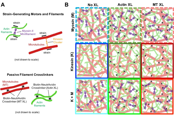
Figure 1. Design and characterization of active actin-microtubule composites with multiple force-generating motors and passive crosslinkers. (A) Actin monomers and tubulin dimers are co-polymerized at molar concentrations c_A and c_T of 0.73-11.6 μM and molar fractions of actin Φ_A = c_A / (c_A + c_T) = 0, 0.25, 0.5, 0.75, and 1, to form co-entangled networks of actin filaments (green) and microtubules (red). Passive crosslinking is achieved using NA to link biotinylated actin filaments (Actin XL) or microtubules (MT XL) at crosslinker:protein molar ratios of R_A = 0.01-0.08 and R_MT = 0.001-0.01 for actin and microtubules, respectively. Myosin-II mini-filaments (purple) and kinesin clusters (orange), at concentrations of c_M = 0.12 - 0.48 μM and c_K = 0.2 - 0.7 μM, push and pull on the filaments to drive the composites out of steady-state. (B) Schematic of formulation space. Myosin II mini-filaments (M), kinesin clusters (K), or both motors (K+M) are incorporated into composites with no passive crosslinkers (No XL), actin-actin crosslinks (Actin XL), and microtubule-microtubule crosslinks (MT XL). All cartoons are not drawn to scale. Please click here to view a larger version of this figure.

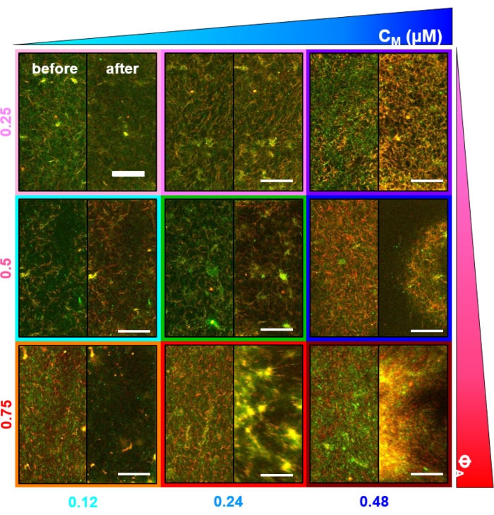
Figure 2. Two-color confocal imaging of myosin-driven cytoskeleton composites with varying myosin concentrations c_M and molar actin fractions Φ_A. (A) 256 x 128 square-pixel (212 x 106 μm²) two-color confocal microscopy images show how composites of actin filaments (green) and microtubules (red) are rearranged via myosin motor activity. No kinesin motors or passive crosslinkers are present. In each panel, images taken at the beginning (left, before) and end (right, after) of the 45 min myosin activation (via illumination with 488 nm light to deactivate blebbistatin) are shown. Panels are ordered by increasing molar concentration of myosin (c_M), going from left to right, and increasing molar fraction of actin (Φ_A), going from top to bottom. The colors outlining each panel match the color coding used in Figure 4 and Figure 5. Scale bars are 50 μM. To best capture dynamics and structure for analysis, we use frame rates of 1-5 fps, ROIs with 50-250 µm sides, and time-series durations of 5-45 min, depending on the rate of contraction and rearrangement. Panels in which the before and after images look similar indicate minimal restructuring, as seen in the pink, magenta, and cyan panels. Small-scale clustering, evidenced by increased heterogeneity and the presence of bright punctate features, can be seen in the orange, green, and red panels. Large-scale contraction, seen as a uniformly shrinking network, is evident in the blue and purple panels. This figure has been modified from reference¹⁷. Please click here to view a larger version of this figure.

Figure 3. Particle image velocimetry (PIV) shows that actomyosin activity triggers coordinated contractile dynamics of actin and microtubules in co-entangled composites. PIV flow fields for actin (top row) and microtubules (bottom row) in a myosin-driven composite with (Φ_A, c_M) = (0.5, 0.24) at increasing times during a 6 min time-series. Flow fields were generated using the Fiji/ImageJ PIV plugin with a lag-time of 20 s and 2 pixel x 2 pixel binning. Both actin and microtubules show consistent motion directed towards the center region of the field-of-view throughout the movie duration. Scale bars in all images are 50 μm. Different arrow colors correspond to different speeds as indicated in the color scale to the right of vector fields. This figure has been modified from reference²⁶. Please click here to view a larger version of this figure.

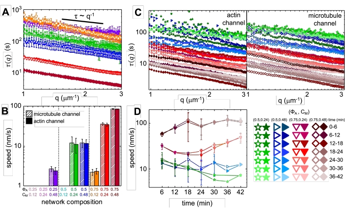
Figure 4. Time-resolved differential dynamic microscopy (DDM) measures the rate and type of motion of actin and microtubules in active composites. (A) DDM is performed on microtubule (top, open symbols) and actin (bottom, filled symbols) channels of time-series to determine characteristic decay times τ vs wavenumber q for both actin (filled symbols) and microtubules (open symbols) as described previously^17,26. All curves follow τ ~ q^-1 scaling, indicating ballistic motion, with speeds v that are determined via fits to τ(q) = (vq)^-1. Faster speeds correspond to smaller τ(q) values for any given q. Symbol colors and shapes correspond to (Φ_A, c_M) combinations shown in B. (B) Contraction speeds v are determined via fits to τ(q) curves shown in A, which are averaged over all lag-times for the duration of each 45 min time-series. (C) Time-resolved DDM (trDDM) quantifies how the dynamics vary over time by evaluating τ(q) for actin (filled symbols, left) and microtubules (open symbols, right) for consecutive 6 min intervals (denoted by different shades of the same color) during the 45 min activation time. trDDM is performed for each (Φ_A, c_M) combination (denoted by different symbols and colors) as described in the legend in lower right. τ(q) curves shown in C follow similar scaling and trends as those in A but also show time-dependence for certain (Φ_A, c_M) compositions, most notably for Φ_A = 0.75. (D) Contraction speeds for actin filaments (closed symbols) and microtubules (open symbols) are determined from fits to corresponding τ(q) curves. Error bars in all plots represent the standard error of values across three to five replicates. This figure has been modified from reference¹⁷. Please click here to view a larger version of this figure.

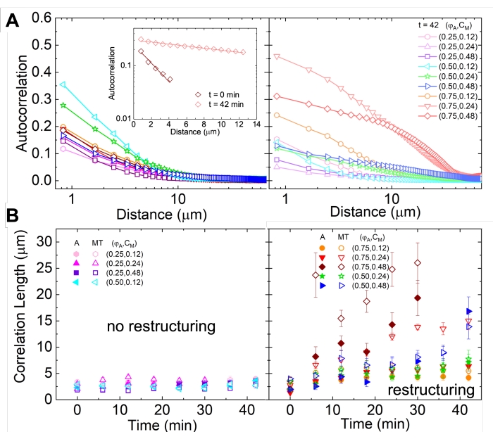
Figure 5. Spatial image autocorrelation (SIA) analysis quantifies the motor-driven restructuring of active cytoskeletal composites. (A) Autocorrelation g(r) for the microtubules at the beginning (left, t = 0 min, dark shades) and end (right, t = 42 min, light shades) of the experiment for (Φ_A, c_M) formulations listed in the legend. Inset: example fits of data to  at the initial and final times for (Φ_A, c_M) = (0.75, 0.12). (B) Average correlation lengths ξ for actin (closed symbols) and microtubules (open symbols) for each (Φ_A, c_M) determined via exponential fits of each g(r) curve, as shown in the inset in A. Data is divided into those that exhibit minimal (left) versus substantial (right) restructuring. Error bars in A and B represent the standard error across three to five replicates. This figure has been modified from reference¹⁷. Please click here to view a larger version of this figure.

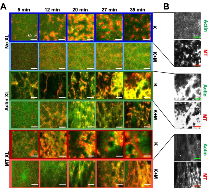
Figure 6. Incorporating kinesin motors and passive crosslinkers into active composites to increase programmability and expand the phase space of dynamics and structure. (A) Two-color confocal images of actin (green) and microtubules (red) in active composites show complex formulation-dependent restructuring over time (listed in min). The five images in each row correspond to five frames of a 2000 frame time-series acquired for a composite driven by kinesin (K, rows 1, 3, 5) or kinesin and myosin (K+M, rows 2, 4, 6), and including either no passive crosslinkers (No XL, rows 1, 2), actin-actin crosslinks (Actin XL, rows 3, 4), or microtubule-microtubule crosslinks (MT XL, rows 5, 6). Scale bars are all 50 µm. Outline colors match color scheme in Figure 8. (B) Separate actin and microtubule fluorescence channels for the kinesin-only composites show varied structures with both actin-MT co-localization and micro-phase separation. The images shown are for composites with c_A = 2.32 μM, c_T = 3.48 μM, c_K = 0.35 μM, c_M = 0.47 μM (rows 2, 4, 6), R_A = 0.02 (rows 3, 4), and R_MT = 0.005 (rows 5, 6). All composites begin with uniformly distributed interpenetrating networks of actin and microtubules (column 1). Kinesin-driven composites without crosslinkers (row 1) form loosely connected amorphous clusters that are MT-rich. Actin co-localizes in the centers of these aggregates initially but then is squeezed out of the MT-rich regions that continue to contract and disconnect from one another. Actin-actin crosslinking (row 3) hinders this microscale actin-MT separation, and instead MT-rich aggregates are connected via long strands of actin. Actin crosslinking also enables slow uptake of actin into the MT-rich regions, such that the composite becomes a connected network of co-localized actin and MT clusters. Microtubule crosslinking (row 5) leads to amorphous clustering of MTs that coalesce over time, resulting in larger scale phase separation of actin and MTs. Adding myosin (rows 2, 4, 6) reduces kinesin-driven de-mixing and restructuring. Without crosslinkers (row 2), composites show little rearrangement over the course of hours. Crosslinking increases restructuring and co-localization of actin and microtubules (rows 4, 6). Specifically, when microtubules are crosslinked (row 6), there is significant interpenetration and reorganization into web-like networks of fibers. This figure has been modified from reference⁵⁰. Please click here to view a larger version of this figure.

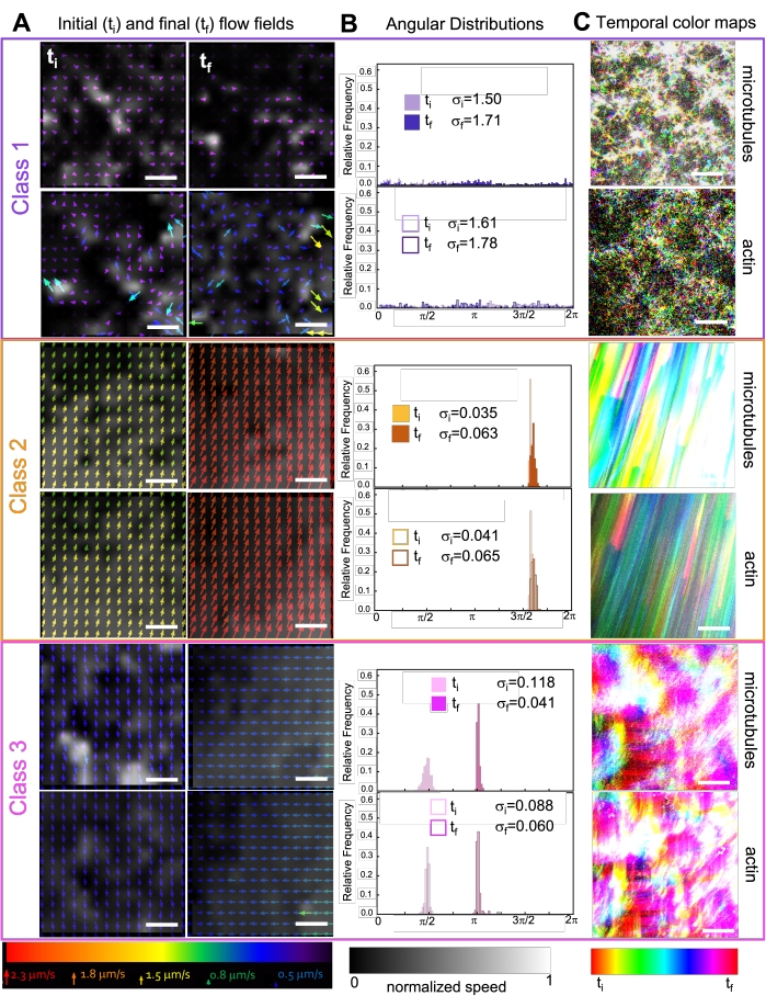
Figure 7. PIV shows that active composites exhibit three classes of spatiotemporally distinct flow fields. (A) PIV flow fields for the first (t_i) and last (t_f) frames of three representative time-series, showing the different dynamical classes that composites shown in Figure 6 exhibit. PIV flow fields for microtubules (top) and actin (bottom) for class 1 (top, purple), class 2 (middle, orange), and class 3 (bottom, magenta) example videos, with arrow colors corresponding to the universal speed scale at the bottom, and the grayscale colormap showing the spatial speed distribution, normalized separately for each flow field according to the scale shown at bottom. Scale bars are all 50 μM. (B) Angular distributions of velocity vectors from A (in units of radians) with listed initial and final standard deviations σ_i and σ_f. (C) Temporal color maps for the videos analyzed in A and B show the frame-to-frame position of each pixel relative to its starting point. Class 1 maps show small-scale random motion; class 2 maps depict fast unidirectional motion with minimal spatial or temporal variation; class 3 maps exhibit features of both class 1 and 2. This figure has been modified from reference⁵⁰. Please click here to view a larger version of this figure.

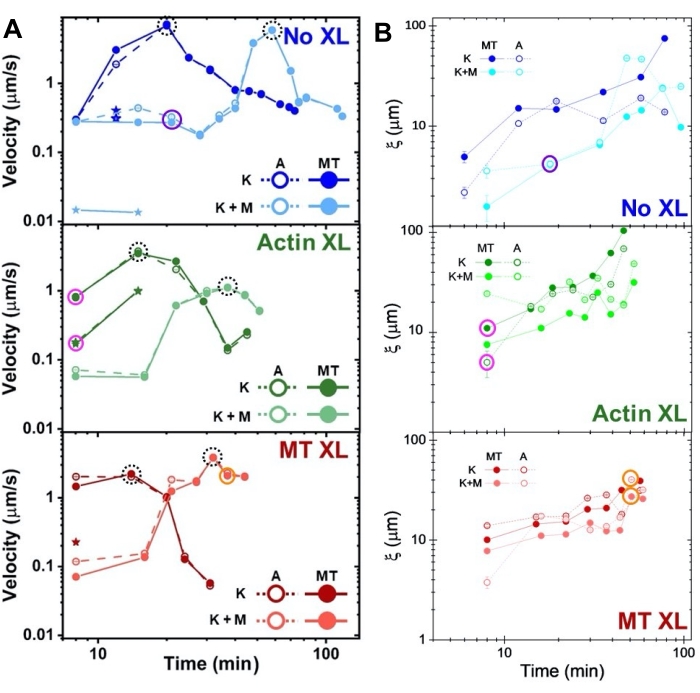
Figure 8. DDM and SIA measure the time-varying dynamics and structure of two-motor actin-microtubule composites. (A) Speeds for composites described in Figure 6 and Figure 7, measured via DDM, show acceleration and deceleration of composites, programmed by crosslinking and myosin activity. Speeds of microtubules (MT, closed circles) and actin (A, open circles) are plotted as a function of activity time in composites with no crosslinking (top, blue), actin crosslinking (middle, green), microtubule crosslinking (bottom, red), without myosin (K, darker shades), and with myosin (K+M, lighter shades). For class 3 cases, which have two speeds, the slower speed is indicated by a star. Data points enclosed by dashed black circles correspond to maximum speed v_max for each formulation. Error bars (most too small to see) are the standard error over the power-law fits of the corresponding τ(q). (B) Structural correlation lengths ξ, determined via SIA, versus activity time, for the same set of time-series evaluated in A. Each data point is an average of the correlation lengths determined for the first and last frame of the corresponding time-series. In general, ξ increases in time for both actin and microtubules in all composites systems, and composites driven solely by kinesin have greater correlation lengths than those in which myosin is also present. Data points in A and B that correspond to the three time-series analyzed in Figure 7 are circled in the corresponding class color (1 = purple, 2 = orange, 3 = magenta). This figure has been modified from reference⁵⁰. Please click here to view a larger version of this figure.

Discussion

A key advance of the reconstituted system described above is its modularity and tunability, so users are encouraged to modify the concentrations of proteins, motors, crosslinkers, etc. to suit their desired outcomes, whether it be to emulate a particular cellular process or engineer a material with specific functionality or mechanical properties. Limitations on the concentration range of actin and tubulin are set at the lower limit by the critical concentration needed to polymerize actin (~0.2 μM)^57,58,59 and tubulin (~3 - 4 μM)⁶⁰, and at the upper limit by the transition to nematic alignment of actin filaments (~90 μM)^61,62 or microtubules (~35 μM)⁶³. Actin monomers and tubulin dimers should be polymerized into filaments together, rather than mixed together after polymerization, to ensure that they form homogenously interpenetrating percolated networks that synergistically support each other. The novel dynamics that the composites exhibit rely on this interaction. While it is generally important to follow all steps as outlined in the protocol to successfully reproduce the results shown, some steps are more exacting, while others have room to modify and adjust to fit specific needs and available resources.

For example, one important step in ensuring reproducible results is properly preparing and storing the reagents following the guidelines provided in the Table of Materials. Cytoskeletal proteins (actin, tubulin, myosin, kinesin) are labile and should be aliquoted, flash-frozen with liquid nitrogen, and stored at -80 °C in single-use aliquots. Once removed from -80 °C, aliquots should be kept on ice. Cytoskeletal proteins do not reliably retain function after additional freeze-thaw cycles.

Microtubules are more sensitive to depolymerization and denaturing than actin. Once removed from -80 °C, tubulin should be kept on ice before polymerization, and used within 12 h. Once polymerized, microtubules should be kept at room temperature. It is also critical to stabilize microtubules with taxol to prevent depolymerization. Phalloidin-stabilization of actin filaments is likewise important to suppress the ATP-consuming actin treadmilling that competes with myosin and kinesin activity.

Ultracentrifugation of myosin motors is another critical step, as it removes inactive myosin dead heads. Not removing the enzymatically inactive monomers results in passive crosslinking of the actin network and loss of activity. To prolong ATPase activity of motors, an ATP regeneration system such as creatine phosphate and creatine phosphokinase⁶⁴ can be incorporated.

Finally, maintaining composite activity requires inhibiting adsorption of filaments and motors to the walls of the sample chamber, which can be achieved by passivation of the microscope coverslips and slides. Motor proteins are particularly prone to adsorption, which results in the composite being pulled to the surface of the sample chamber, moving out of the field-of-view, collapsing to 2D, and no longer undergoing activity. Silanizing the coverslips and slides is an effective way to passivate the surfaces and prevent adsorption (see step 1). An alternative passivation method used effectively in in vitro cytoskeleton experiments is coating the surface with a lipid bilayer, similar to the cell membrane¹⁸. This method is advantageous if one wishes to tether proteins to the surface or introduce other specific protein-surface interactions, because the bilayer can be functionalized. For optical tweezers experiments, passivation of the microspheres is also critical, and can be achieved by coating carboxylated microspheres with BSA or PEG via carbodiimide crosslinker chemistry⁴⁸.

There are a few aspects of the presented protocols that researchers may consider altering to suit their needs. Firstly, researchers may choose to replace non-native biotin-NA crosslinkers with biological crosslinkers, such as alpha-actinin or MAP65 that crosslink actin and microtubules, respectively^28,65,66. The use of non-native crosslinkers in the composites described here is motivated by their enhanced reproducibility, stability, and tunability compared to native crosslinkers. Because of the strong biotin-NA bond, crosslinkers can be assumed to be permanent, rather than most native crosslinkers that transiently bind with wide-ranging turnover rates. The dynamics of transient crosslinking complicates parsing the contributions from crosslinkers and motors to the dynamics. Moreover, biotin-NA linkers can be versatilely used to crosslink both actin and microtubules, as well as crosslink actin to microtubules. In this way, an unambiguous comparison between crosslinking motifs can be made, keeping all other variables (e.g., crosslinker size, binding affinity, stoichiometry, etc.) fixed. Finally, the reagents needed to incorporate biotin-NA linkers are widely commercially available, well-characterized, and commonly used in many biophysics labs. However, one of the key strengths of the in vitro platform described here is its modularity, so researchers should be able to seamlessly replace biotin-NA linkers with native linkers should they choose.

Secondly, in the current protocol, actin monomers and tubulin dimers are polymerized into filaments together in a centrifuge tube prior to adding to the sample chamber. Flowing the solution of entangled filamentous proteins into the sample chamber may cause flow alignment, especially of the microtubules, which breaks the desired isotropy and homogeneity of the composites. Indeed, a major advance in prior work on steady-state actin-microtubule composites was the ability to co-polymerize actin and microtubules in situ (in the sample chamber) to ensure formation of isotropic interpenetrating networks of actin and microtubules^15,16,27. However, extending this approach to active composites would require adding the motors to the sample prior to actin and tubulin polymerization and having the entire sample incubate together at 37 °C prior to experiments. Tests of this variation to the protocol have resulted in reduced actin polymerization and no discernible motor activity, likely due to competing ATPase activity and the prolonged 37 °C incubation of the motors. Fortunately, there is no discernible flow alignment of composites when following the current protocols, as can be seen in Figure 2, Figure 3, and Figure 6. Nevertheless, researchers are encouraged to design protocols that allow for in situ formation of active composites.

Another point of consideration is the fluorescence labeling scheme, which entails sparsely labeling all of the actin filaments and microtubules in the network. This labeling approach was optimized to directly visualize the structure of the network rather than inferring structure and dynamics via tracer filaments or microspheres. However, the tradeoff is that individual filaments are not brightly labeled and resolvable. One approach that researchers could take to both resolve single filaments as well as visualize network structure is to dope in pre-formed filaments labeled with another fluorophore, so both the surrounding network and individual filaments could be imaged simultaneously. However, when using more than two fluorophores and excitation/emission channels, bleed-through between channels is often hard to eliminate, so care must be taken in choosing the fluorophores, filters, and laser intensities.

A related limitation is the inability to visualize the myosin or kinesin motors in the composites. The fluorescent-labeled actin monomers and tubulin dimers used are commercially available, whereas visualization of myosin or kinesin in composites requires in-house labeling. Researchers are encouraged to take the next step to label motors, as done previously^18,67, to be able to unequivocally link motor activity and binding to the dynamics and structures that our composites exhibit.

Finally, it is important to note that, in the current protocol, the onset and duration of kinesin activity is not controlled. Because the myosin activity is controlled using photo-deactivation of blebbistatin, as described above, to build in similar light-activation of kinesin, one can incorporate light-activated ATP.

To build up the complexity of the designs described here, to better mimic cellular conditions and broaden the dynamic-structure-function parameter space, future work will focus on incorporating intermediate filaments, such as vimentin^68,69, as well as other motors such as dynein^13,70. Gelsolin will also be incorporated at different concentrations to control actin length¹⁴, as well as tau protein to control microtubule stiffness.

In summary, the presented protocols describe how to design, create, and characterize the dynamics, structure, and mechanics of cytoskeleton-inspired active matter systems, that contain two separate active force-generating components that act on different substrates in a single system. This tunable and modular platform brings reconstitution efforts one important step closer to mimicking the cellular cytoskeleton and offers the unique ability to program its properties across a wide phase space by independently incorporating, removing, and tuning the different components. Moreover, all components of this versatile system are commercially available (see Table of Materials), except for the kinesin dimers which are purified in the Ross Lab, as described previously⁵⁰, and available upon request. Finally, all analysis code is freely available through GitHub⁴⁹ and is based on free programming languages and software (Python and Fiji). The transparent dissemination of protocols to design these systems will hopefully make this platform more accessible to a diverse group of users with different expertise, backgrounds, institutional affiliations, and research goals.

Materials

List of materials used in this article

Name	Company	Catalog Number	Comments
(-)-Blebbistatin  Abbreviation used in paper: blebbistatin	Sigma Aldrich	B0560	Stock Concentration: 200 μM in DMSO Storage: dessicated, in DMSO, -20ºC Stock and Experiment Recipes: dissolve 1 mg of powder to 200 μM in DMSO Storage, Handling, Troubleshooting Notes: limited shelf-life, typically stops functioning reliably after 3-4 months. purchase and prepare new solution every 3 months.
1:20 488-tubulin:tubulin mixture  Abbreviation used in paper: 5-488-tubulin	NA	NA	Stock Concentration: 5 mg/ml in PEM Storage: single use aliquots, -80ºC, avoid freeze-thaw cycles Stock and Experiment Recipes: mix tubulin and 488-tubulin at a 20:1 ratio, flash freeze with LN2 Storage, Handling, Troubleshooting Notes: each aliquot can be used for up to 12 hrs stored on ice at 4ºC, protect from light
1:20 R-tubulin:tubulin mixture  Abbreviation used in paper: 5-R-tubulin	NA	NA	Stock Concentration: 5 mg/ml in PEM Storage: single use aliquots, -80ºC, avoid freeze-thaw cycles Stock and Experiment Recipes: mix tubulin and rhodamine tubulin at a 20:1 ratio, flash freeze with LN2 Storage, Handling, Troubleshooting Notes: each aliquot can be used for up to 12 hrs stored on ice at 4ºC, protect from light
actin (biotin): skeletal muscle  Abbreviation used in paper: biotin-actin	Cytoskeleton	AB07	Stock Concentration: 1 mg/ml in G-buffer Storage: single use aliquots, -80ºC, avoid freeze-thaw cycles Stock and Experiment Recipes: reconstitute to 1 mg/ml in G-buffer, flash freeze with LN2 Storage, Handling, Troubleshooting Notes: (1) immediately prior to use dilute to 0.5 mg/ml in PEM, (2) once removed from -80ºC, store  aliquot on ice at 4ºC for up to 1 week
actin (rhodamine): rabbit skeletal muscle  Abbreviation used in paper: R-actin	Cytoskeleton	AR05	Stock Concentration: 1.5 mg/ml in G-buffer Storage: single use aliquots, -80ºC, avoid freeze-thaw cycles Stock and Experiment Recipes: reconstitute to 1.5 mg/ml in G-buffer, flash freeze with LN2 Storage, Handling, Troubleshooting Notes: once removed from -80ºC, store  aliquot on ice at 4ºC, can be used for up to 1 week
adenosine triphosphate  Abbreviation used in paper: ATP	Thermo Fisher Scientific	A1048	Stock Concentration: 100 mM Storage: in solution (pH 7), -20ºC Stock and Experiment Recipes: reconsitute in DI H20, bring pH to 7 with NaOH Storage, Handling, Troubleshooting Notes: routinely check pH and adjust as needed, hydrolyzes over time, replace every ~6-12 months
AlexaFluor488 Phalloidin  Abbreviation used in paper: 488-phalloidin	Thermo Fisher Scientific	A12379	Stock Concentration: 100 μM DMSO Storage: protected from light, dessicated, -20ºC Stock and Experiment Recipes: reconstitute to 100 μM with DMSO Storage, Handling, Troubleshooting Notes: immediately prior to use dilute to 20 μM in PEM (1 μL in 4 μL PEM)
AlexaFluor488–labeled actin  Abbreviation used in paper: 488-actin	Thermo Fisher Scientific	A12373	Stock Concentration: 1.5 mg/ml in G-buffer Storage: single use aliquots, -80ºC, avoid freeze-thaw cycles Stock and Experiment Recipes: reconstitute to 1.5 mg/ml in G-buffer, flash freeze with LN2 Storage, Handling, Troubleshooting Notes: this item has been discontinued
Basic Plasma Cleaner  Abbreviation used in paper: plasma cleaner	Harrick Plasma	PDC-32G
Bemis Parafilm M Laboratory Wrapping Film  Abbreviation used in paper: transparent film	Thermo Fisher Scientific	13-374-5
D-(+)-Glucose  Abbreviation used in paper:	Thermo Fisher Scientific	A1682836	Stock Concentration: 100x Storage: store at stock concentration (100x) or 10x concentration, dessicated, at -20ºC Stock and Experiment Recipes: reconstitute powder to 4.5 mg/ml in DI H20 Storage, Handling, Troubleshooting Notes: final concentration in solution should 45 μg/mL
D-Biotin  Abbreviation used in paper: biotin	Fisher Scientific	BP232-1	Stock Concentration: 1.02 mM in PEM Storage: dessicated, 4ºC
deionized nanopure water  Abbreviation used in paper: DI
Dimethyldichlorosilane  Abbreviation used in paper: silane	Thermo Fisher Scientific	D/3820/PB05	Stock Concentration: 2% dissolved in Toulene
Dithiothreitol  Abbreviation used in paper: DTT	Thermo Fisher Scientific	R0861	Stock Concentration: 1 M in DMSO Storage: dessicated, -20ºC Stock and Experiment Recipes: dilute to 2 mM in PEM immediately before each experiment
DMSO Anhydrous  Abbreviation used in paper: DMSO	Thermo Fisher Scientific	D12345
F-Buffer  Abbreviation used in paper: F-buffer	NA	NA	Stock Concentration: 10x Storage: dessicated, -20ºC Stock and Experiment Recipes: 10 mM Imidazole (pH 7.0), 50 mM KCl, 1 mM MgCl2, 1 mM EGTA, 0.2 mM ATP
G-Buffer  Abbreviation used in paper: G-buffer	NA	NA	Stock Concentration: 10x Storage: dessicated, -20ºC Stock and Experiment Recipes: 2.0 mM Tris (pH 8), 0.2 mM ATP, 0.5 mM DTT, 0.1 mM CaCl2. Store at -20°C.
glass microscope slide  Abbreviation used in paper: slide	Thermo Fisher Scientific	22-310397
Glucose oxidase + catalase + β-mercaptoethanol  Abbreviation used in paper: GOC	Sigma Aldrich	G2133-250KU, C1345, 63689	Stock Concentration: 100x Storage: store at stock concentration (100x) or 10x concentration, dessicated, at -20ºC Stock and Experiment Recipes: For 100x: 4.3 mg/ml glucose oxidase, 0.7 mg/ml catalase, 0.5% v/v  β-mercaptoethanol in DI H20 Storage, Handling, Troubleshooting Notes: final concentration in solution should be: 0.005% β-mercaptoethanol, 43 μg/mL glucose oxidase, 7 μg/mL catalase
glu-GOC oxygen scavenging system  Abbreviation used in paper: glu-GOC	NA	NA	Stock Concentration: 100x Storage: prepare fresh each time Stock and Experiment Recipes: mix equal parts Glu and GOC and add at 1/100 final sample volume immediately before imaging Storage, Handling, Troubleshooting Notes: prepare from Glu and GOC immediately before imaging
Guanosine triphosphate  Abbreviation used in paper: GTP	Thermo Fisher Scientific	R0461	Stock Concentration: 100 mM Storage: 100 μL aliquots at -20ºC
Instant Mix 1-minute epoxy  Abbreviation used in paper: epoxy	Loctite	1366072
Kinesin-1 401 BIO 6x HIS  Abbreviation used in paper: kinesin	Prepared in JL Ross Lab at Syracuse University	NA	Stock Concentration: 8.87 μM in PEM Storage: single use aliquots, -80ºC, avoid freeze-thaw cycles Storage, Handling, Troubleshooting Notes: biotinylated dimers form kinesin clusters, each aliquot can be used for up to 12 hrs stored on ice at 4ºC
NeutrAvidin  Abbreviation used in paper: NA	Thermo Fisher Scientific	31000	Stock Concentration: 5 mg/ml in PEM Storage: dessicated, -20ºC Stock and Experiment Recipes: reconstitute powder to 5 mg/ml in PEM
No 1. glass coverslips (24 mm x 24 mm)  Abbreviation used in paper: coverslip	Thermo Fisher Scientific	12-548-CP
Paclitaxel   Abbreviation used in paper: Taxol	Thermo Fisher Scientific	P3456	Stock Concentration: 2 mM in DMSO Storage: protected from light, dessicated, -20ºC Stock and Experiment Recipes: reconstitute to 2 mM with DMSO Storage, Handling, Troubleshooting Notes: immediately prior to use dilute to 200 μM in DMSO (0.4 μL in 3.6 μL DMSO)
PEM-100  Abbreviation used in paper: PEM	NA	NA	Stock Concentration: 1x Storage: room temperature (RT) Stock and Experiment Recipes: 100 mM K-PIPES (pH 6.8), 2 mM EGTA, 2 mM MgCl2 Storage, Handling, Troubleshooting Notes: use KOH to adjust pH to 6.8, recheck pH often and adjust accordingly
phalloidin Abbreviation used in paper: phalloidin	Thermo Fisher Scientific	P3457	Stock Concentration: 100 μM in DMSO Storage: protected from light, dessicated, -20ºC, adhere closely to storage/handling conditions Stock and Experiment Recipes: reconstitute to 100 μM with DMSO Storage, Handling, Troubleshooting Notes: susceptible to impurities in its preparation and denaturing, identifiable as large amorphous aggregates of actin in samples
porcine brain tubulin  Abbreviation used in paper: tubulin	Cytoskeleton	T240	Stock Concentration: 5 mg/ml in PEM Storage: single use aliquots, -80ºC, avoid freeze-thaw cycles Stock and Experiment Recipes: reconstitute powder to 5 mg/ml in PEM, flash freeze with LN2 Storage, Handling, Troubleshooting Notes: each aliquot can be used for up to 12 hrs stored on ice at 4ºC
Potassium Chloride  Abbreviation used in paper: KCl	Thermo Fisher Scientific	AM9640G	Stock Concentration: 4 M Storage: RT
Rabbit skeletal actin  Abbreviation used in paper: actin	Cytoskeleton	AKL99	Stock Concentration: 2 mg/ml in G-buffer Storage: single use aliquots, -80ºC, avoid freeze-thaw cycles Stock and Experiment Recipes: reconstitute to 2 mg/ml in G-buffer, flash freeze with LN2 Storage, Handling, Troubleshooting Notes: once removed from -80ºC, store  aliquot on ice at 4ºC, can be used for up to 1 week
Rabbit skeletal myosin II  Abbreviation used in paper: myosin	Cytoskeleton	MY02	Stock Concentration: 10 mg/ml in PEM Storage: single use aliquots, -80ºC, avoid freeze-thaw cycles Stock and Experiment Recipes: reconstitute powder to 10 mg/ml in PEM, flash freeze with LN2 Storage, Handling, Troubleshooting Notes: monomers form minifilaments at low KCl, each aliquot can be used for up to 12 hrs stored on ice at 4ºC
Tubulin (biotin): porcine brain  Abbreviation used in paper: biotin-tubulin	Cytoskeleton	T333P	Stock Concentration: 5 mg/ml in PEM Storage: single use aliquots, -80ºC, avoid freeze-thaw cycles Stock and Experiment Recipes: reconstitute powder to 5 mg/ml in PEM, flash freeze with LN2 Storage, Handling, Troubleshooting Notes: immediately prior to use dilute to 0.5 mg/ml in PEM
Tubulin (fluorescent HiLyte 488): porcine brain  Abbreviation used in paper: 488-tubulin	Cytoskeleton	TL488M	Stock Concentration: 5 mg/ml in PEM Storage: single use aliquots, -80ºC, avoid freeze-thaw cycles Stock and Experiment Recipes: reconstitute powder to 5 mg/ml in PEM, flash freeze with LN2 Storage, Handling, Troubleshooting Notes: each aliquot can be used for up to 12 hrs stored on ice at 4ºC, protect from light
tubulin (rhodamine): porcine brain  Abbreviation used in paper: R-tubulin	Cytoskeleton	TL590M	Stock Concentration: 5 mg/ml in PEM Storage: single use aliquots, -80ºC, avoid freeze-thaw cycles Stock and Experiment Recipes: reconstitute powder to 5 mg/ml in PEM, flash freeze with LN2 Storage, Handling, Troubleshooting Notes: each aliquot can be used for up to 12 hrs stored on ice at 4ºC, protect from light
Tween 20  Abbreviation used in paper: Tween20	Thermo Fisher Scientific	J20605.AP	Stock Concentration: 1% v/v in DI H20 Storage: RT
ultracentrifuge grade microtubes  Abbreviation used in paper: Beckman-Coulter Optima Max XP	Beckman Coultier	343776	Storage, Handling, Troubleshooting Notes: 8x34 mm PC
UV light curing glue  Abbreviation used in paper: UV glue	Pharda	SKG-2869

References

- Fletcher, D. A., Mullins, R. D. Cell mechanics and the cytoskeleton. Nature. 463 (7280), 485-492 (2010).
- Koenderink, G. H., Paluch, E. K. Architecture shapes contractility in actomyosin networks. Current Opinion in Cell Biology. 50, 79-85 (2018).
- Dogterom, M., Koenderink, G. H. Actin-microtubule crosstalk in cell biology. Nature Reviews Molecular Cell Biology. 20 (1), 38-54 (2019).
- Burla, F., Mulla, Y., Vos, B. E., Aufderhorst-Roberts, A., Koenderink, G. H. From mechanical resilience to active material properties in biopolymer networks. Nature Reviews Physics. 1 (4), 249-263 (2019).
- Wen, Q., Janmey, P. A. Polymer physics of the cytoskeleton. Current Opinion in Solid State and Materials Science. 15 (5), 177-182 (2011).
- Xiao, Q., Hu, X., Wei, Z., Tam, K. Y. Cytoskeleton molecular motors: structures and their functions in neuron. International Journal of Biological Sciences. 12 (9), 1083-1092 (2016).
- Ajeti, V. et al. Wound healing coordinates actin architectures to regulate mechanical work. Nature Physics. 15 (7), 696-705 (2019).
- Jung, W. et al. Dynamic motions of molecular motors in the actin cytoskeleton. Cytoskeleton. 76 (11-12), 517-531 (2019).
- Pollard, T. D., O'Shaughnessy, B. Molecular mechanism of cytokinesis. Annual Review of Biochemistry. 88 (1), 661-689 (2019).
- Huber, F., Boire, A., López, M. P., Koenderink, G. H. Cytoskeletal crosstalk: when three different personalities team up. Current Opinion in Cell Biology. 32, 39-47 (2015).
- Rivero, F. et al. The role of the cortical cytoskeleton: F-actin crosslinking proteins protect against osmotic stress, ensure cell size, cell shape and motility, and contribute to phagocytosis and development. Journal of Cell Science. 109 (11), 2679-2691 (1996).
- Duclos, G. et al. Topological structure and dynamics of three-dimensional active nematics. Science. 367 (6482), 1120-1124 (2020).
- Baclayon, M. et al. Optical tweezers-based measurements of forces and dynamics at microtubule ends. Optical Tweezers. 1486, 411-435 (2017).
- Gurmessa, B., Fitzpatrick, R., Falzone, T. T., Robertson-Anderson, R. M. Entanglement density tunes microscale nonlinear response of entangled actin. Macromolecules. 49 (10), 3948-3955 (2016).
- Francis, M. L. et al. Non-monotonic dependence of stiffness on actin crosslinking in cytoskeleton composites. Soft Matter. 15 (44), 9056-9065 (2019).
- Ricketts, S. N. et al. Varying crosslinking motifs drive the mesoscale mechanics of actin-microtubule composites. Scientific Reports. 9 (1), 12831 (2019).
- Lee, G. et al. Active cytoskeletal composites display emergent tunable contractility and restructuring. Soft Matter. 17 (47), 10765-10776 (2021).
- Murrell, M. P., Gardel, M. L. F-actin buckling coordinates contractility and severing in a biomimetic actomyosin cortex. Proceedings of the National Academy of Sciences. 109 (51), 20820-20825 (2012).
- Soares e Silva, M. et al. Active multistage coarsening of actin networks driven by myosin motors. Proceedings of the National Academy of Sciences. 108 (23), 9408-9413 (2011).
- Sonn-Segev, A., Bernheim-Groswasser, A., Roichman, Y. Dynamics in steady state in vitro acto-myosin networks. Journal of Physics: Condensed Matter. 29 (16), 163002 (2017).
- Ideses, Y., Sonn-Segev, A., Roichman, Y., Bernheim-Groswasser, A. Myosin II does it all: assembly, remodeling, and disassembly of actin networks are governed by myosin II activity. Soft Matter. 9 (29), 7127 (2013).
- Fürthauer, S. et al. Self-straining of actively crosslinked microtubule networks. Nature Physics. 15 (12), 1295-1300 (2019).
- Lemma, L. M. et al. Multiscale microtubule dynamics in active nematics. Physical Review Letters. 127 (14), 148001 (2021).
- Fan, Y., Wu, K.-T., Aghvami, S. A., Fraden, S., Breuer, K. S. Effects of confinement on the dynamics and correlation scales in kinesin-microtubule active fluids. Physical Review E. 104 (3), 034601 (2021).
- Triclin, S. et al. Self-repair protects microtubules from destruction by molecular motors. Nature Materials. 20 (6), 883-891 (2021).
- Lee, G. et al. Myosin-driven actin-microtubule networks exhibit self-organized contractile dynamics. Science Advances. 7 (6), eabe4334 (2021).
- Ricketts, S. N., Ross, J. L., Robertson-Anderson, R. M. Co-entangled actin-microtubule composites exhibit tunable stiffness and power-law stress relaxation. Biophysical Journal. 115 (6), 1055-1067 (2018).
- Bendix, P. M. et al. A quantitative analysis of contractility in active cytoskeletal protein networks. Biophysical Journal. 94 (8), 3126-3136 (2008).
- Linsmeier, I. et al. Disordered actomyosin networks are sufficient to produce cooperative and telescopic contractility. Nature Communications. 7 (1), 12615 (2016).
- Stam, S. et al. Filament rigidity and connectivity tune the deformation modes of active biopolymer networks. Proceedings of the National Academy of Sciences. 114 (47), E10037-E10045 (2017).
- Yadav, V. et al. Filament nucleation tunes mechanical memory in active polymer networks. Advanced Functional Materials. 29 (49), 1905243 (2019).
- Ennomani, H. et al. Architecture and connectivity govern actin network contractility. Current Biology. 26 (5), 616-626 (2016).
- Alvarado, J., Sheinman, M., Sharma, A., MacKintosh, F. C., Koenderink, G. H. Molecular motors robustly drive active gels to a critically connected state. Nature Physics. 9 (9), 591-597 (2013).
- Alvarado, J., Cipelletti, L., Koenderink, G. H. Uncovering the dynamic precursors to motor-driven contraction of active gels. Soft Matter. 15 (42), 8552-8565 (2019).
- Jung, W., Murrell, M. P., Kim, T. F-actin cross-linking enhances the stability of force generation in disordered actomyosin networks. Computational Particle Mechanics. 2 (4), 317-327 (2015).
- Lenz, M., Thoresen, T., Gardel, M. L., Dinner, A. R. Contractile units in disordered actomyosin bundles arise from f-actin buckling. Physical Review Letters. 108 (23), 238107 (2012).
- Memarian, F.L. et al. Active nematic order and dynamic lane formation of microtubules driven by membrane-bound diffusing motors. Proceedings of the National Academy of Sciences. 118 (52), e2117107118 (2021).
- Needleman, D., Dogic, Z. Active matter at the interface between materials science and cell biology. Nature Reviews Materials. 2 (9), 17048 (2017).
- Foster, P. J., Fürthauer, S., Shelley, M. J., Needleman, D. J. Active contraction of microtubule networks. eLife. 4, e10837 (2015).
- Thijssen, K. et al. Submersed micropatterned structures control active nematic flow, topology, and concentration. Proceedings of the National Academy of Sciences. 118 (38), e2106038118 (2021).
- Sanchez, T., Chen, D. T. N., DeCamp, S. J., Heymann, M., Dogic, Z. Spontaneous motion in hierarchically assembled active matter. Nature. 491 (7424), 431-434 (2012).
- Colen, J. et al. Machine learning active-nematic hydrodynamics. Proceedings of the National Academy of Sciences. 118 (10), e2016708118 (2021).
- Mitchell, K. A., Tan, A. J., Arteaga, J., Hirst, L. S. Fractal generation in a two-dimensional active-nematic fluid. Chaos: An Interdisciplinary Journal of Nonlinear Science. 31 (7), 073125 (2021).
- Pandolfi, R. J., Edwards, L., Johnston, D., Becich, P., Hirst, L. S. Designing highly tunable semiflexible filament networks. Physical Review E. 89 (6), 062602 (2014).
- Tan, A. J. et al. Topological chaos in active nematics. Nature Physics. 15 (10), 1033-1039 (2019).
- Roostalu, J., Rickman, J., Thomas, C., Nédélec, F., Surrey, T. Determinants of polar versus nematic organization in networks of dynamic microtubules and mitotic motors. Cell. 175 (3), 796-808.e14 (2018).
- Ndlec, F. J., Surrey, T., Maggs, A. C., Leibler, S. Self-organization of microtubules and motors. Nature. 389 (6648), 305-308 (1997).
- Sheung, J. Y. et al. Motor-driven restructuring of cytoskeleton composites leads to tunable time-varying elasticity. ACS Macro Letters. 10 (9), 1151-1158 (2021).
- McGorty, R. PyDDM v0.2.0. Zenodo. (2022).
- Achiriloaie, D. H. et al. Kinesin and myosin motors compete to drive rich multi-phase dynamics in programmable cytoskeletal composites. arXiv. (2021).
- Wulstein, D. M., Regan, K. E., Garamella, J., McGorty, R. J., Robertson-Anderson, R. M. Topology-dependent anomalous dynamics of ring and linear DNA are sensitive to cytoskeleton crosslinking. Science Advances. 5 (12), eaay5912 (2019).
- McGorty, R. Image-Correlation. at <https://github.com/rmcgorty/Image-Correlation>. (2020).
- Robertson, C. Theory and practical recommendations for autocorrelation-based image correlation spectroscopy. Journal of Biomedical Optics. 17 (8), 080801 (2012).
- McGorty, R. Differential Dynamic Microscopy - Python. at <https://github.com/rmcgorty/Differential-Dynamic-Microscopy---Python>. (2021).
- Cerbino, R., Trappe, V. Differential dynamic microscopy: probing wave vector dependent dynamics with a microscope. Physical Review Letters. 100 (18), 188102 (2008).
- Robertson-Anderson, R. M. Optical tweezers microrheology: from the basics to advanced techniques and applications. ACS Macro Letters. 7 (8), 968-975 (2018).
- Pollard, T. D. Polymerization of ADP-actin. Journal of Cell Biology. 99 (3), 769-777 (1984).
- Coué, M., Brenner, S. L., Spector, I., Korn, E. D. Inhibition of actin polymerization by latrunculin A. FEBS Letters. 213 (2), 316-318 (1987).
- Pollard, T. D. Actin and actin-binding proteins. Cold Spring Harbor Perspectives in Biology. 8 (8), a018226 (2016).
- Kumar, N. Taxol-induced polymerization of purified tubulin. Mechanism of action. Journal of Biological Chemistry. 256 (20), 10435-10441 (1981).
- Käs, J. et al. F-actin, a model polymer for semiflexible chains in dilute, semidilute, and liquid crystalline solutions. Biophysical Journal. 70 (2), 609-625 (1996).
- Viamontes, J., Narayanan, S., Sandy, A. R., Tang, J. X. Orientational order parameter of the nematic liquid crystalline phase of F -actin. Physical Review E. 73 (6), 061901 (2006).
- Hitt, A. L., Cross, A. R., Williams, R. C. Microtubule solutions display nematic liquid crystalline structure. Journal of Biological Chemistry. 265 (3), 1639-1647 (1990).
- Andexer, J. N., Richter, M. Emerging enzymes for ATP regeneration in biocatalytic processes. ChemBioChem. 16 (3), 380-386 (2015).
- Farhadi, L. et al. Actin and microtubule crosslinkers tune mobility and control co-localization in a composite cytoskeletal network. Soft Matter. 16 (31), 7191-7201 (2020).
- Falzone, T. T., Lenz, M., Kovar, D. R., Gardel, M. L. Assembly kinetics determine the architecture of α-actinin crosslinked F-actin networks. Nature Communications. 3 (1), 861 (2012).
- Thoresen, T., Lenz, M., Gardel, M. L. Reconstitution of contractile actomyosin bundles. Biophysical Journal. 100 (11), 2698-2705 (2011).
- Sanghvi-Shah, R., Weber, G. F. Intermediate filaments at the junction of mechanotransduction, migration, and development. Frontiers in Cell and Developmental Biology. 5, 81 (2017).
- Shen, Y. et al. Effects of vimentin intermediate filaments on the structure and dynamics of in vitro multicomponent interpenetrating cytoskeletal networks. Physical Review Letters. 127 (10), 108101 (2021).
- Laan, L., Roth, S., Dogterom, M. End-on microtubule-dynein interactions and pulling-based positioning of microtubule organizing centers. Cell Cycle. 11 (20), 3750-3757 (2012).
Reprints and Permissions
Erratum
Formal Correction: Erratum: Reconstituting and Characterizing Actin-Microtubule Composites with Tunable Motor-Driven Dynamics and Mechanics
Posted by JoVE Editors on 10/11/2022. Citeable Link.
An erratum was issued for: Reconstituting and Characterizing Actin-Microtubule Composites with Tunable Motor-Driven Dynamics and Mechanics. The Authors section was updated.
Mehrzad Sasanpour1
Daisy H. Achiriloaie1,2
Gloria Lee1
Gregor Leech1
Christopher Currie1
K. Alice Lindsay3
Jennifer L. Ross3
Ryan J. McGorty1
Rae M. Robertson-Anderson1
1Department of Physics and Biophysics, University of San Diego
2W. M. Keck Science Department, Scripps College, Pitzer College, and Claremont McKenna College
3Department of Physics, Syracuse University
to:
Maya Hendija1