AMEBaS: Automatic Midline Extraction and Background Subtraction of Ratiometric Fluorescence Time-Lapses of Polarized Single Cells

Summary

Current methods for analyzing the intracellular dynamics of polarized single cells are often manual and lack standardization. This manuscript introduces a novel image analysis pipeline for automating midline extraction of single polarized cells and quantifying spatiotemporal behavior from time lapses in a user-friendly online interface.

Abstract

Cell polarity is a macroscopic phenomenon established by a collection of spatially concentrated molecules and structures that culminate in the emergence of specialized domains at the subcellular level. It is associated with developing asymmetric morphological structures that underlie key biological functions such as cell division, growth, and migration. In addition, the disruption of cell polarity has been linked to tissue-related disorders such as cancer and gastric dysplasia.

Current methods to evaluate the spatiotemporal dynamics of fluorescent reporters in individual polarized cells often involve manual steps to trace a midline along the cells' major axis, which is time consuming and prone to strong biases. Furthermore, although ratiometric analysis can correct the uneven distribution of reporter molecules using two fluorescence channels, background subtraction techniques are frequently arbitrary and lack statistical support.

This manuscript introduces a novel computational pipeline to automate and quantify the spatiotemporal behavior of single cells using a model of cell polarity: pollen tube/root hair growth and cytosolic ion dynamics. A three-step algorithm was developed to process ratiometric images and extract a quantitative representation of intracellular dynamics and growth. The first step segments the cell from the background, producing a binary mask through a thresholding technique in the pixel intensity space. The second step traces a path through the midline of the cell through a skeletonization operation. Finally, the third step provides the processed data as a ratiometric timelapse and yields a ratiometric kymograph (i.e., a 1D spatial profile through time). Data from ratiometric images acquired with genetically encoded fluorescent reporters from growing pollen tubes were used to benchmark the method. This pipeline allows for faster, less biased, and more accurate representation of the spatiotemporal dynamics along the midline of polarized cells, thus advancing the quantitative toolkit available to investigate cell polarity. The AMEBaS Python source code is available at: https://github.com/badain/amebas.git

Introduction

Cell polarity is a fundamental biological process in which the concerted action of a collection of spatially concentrated molecules and structures culminates in the establishment of specialized morphological subcellular domains¹. Cell division, growth and migration rely on such polarity sites, while its loss has been associated with cancer in epithelial tissue-related disorders².

Apically growing cells are a dramatic example of polarity, where the polarity site at the tip typically reorients to extracellular cues³. These include developing neurites, fungal hyphae, root hairs, and pollen tubes, where multiple cellular processes show pronounced differences from the tip of the cell toward the shank. In pollen tubes, in particular, actin polymerization, vesicle trafficking, and ionic concentrations are markedly polarized, showing tip-focused gradients⁴. Pollen tubes are the male gametophytes of flowering plants and are responsible for delivering the sperm cells to the ovule by growing exclusively at the apex of the cell at one of the fastest growth rates known for a single cell. The tip-focused gradients of ions such as calcium⁵ (Ca²⁺) and protons⁶ (H⁺) play a major role in sustaining pollen tube growth, which is essential to accomplish its main biological function that culminates in a double fertilization^5,6. Thus, quantitative methods to analyze the spatiotemporal dynamics along the midline of apically growing cells are essential to investigate the cellular and molecular mechanisms underlying polarized growth^7,8,9. Researchers often use kymographs, i.e., a matrix that represents the pixel intensities of the cell's midline (e.g., columns) through time (e.g., rows), which allows visualizing cell growth and migration in the diagonal (Figure 1). Despite their usefulness, kymographs are frequently extracted by manually tracing the midline, being prone to biases and human errors while also being rather laborious. This calls for an automated method of midline extraction that is the first feature of the pipeline introduced herein named AMEBaS: Automatic Midline Extraction and Background Subtraction of ratiometric fluorescence time lapses of polarized single cells.

In terms of experimental procedures, quantitative imaging of ions/molecules/species of interest in single cells can be achieved with genetically encoded fluorescent probes¹⁰. Among the ever-expanding choices, ratiometric probes are one of the most accurate since they emit different fluorescence wavelengths when bound/unbound to the molecules of interest¹¹. This allows for correction of the spatial heterogeneity in the intracellular concentration of the probe by using the ratio of two channels with their channel specific background subtracted. However, estimating the background threshold for each channel and time point can be a complex task since it often varies in space due to effects like shading, where the corners of the image have luminosity variation relative to the center, and in time due to fading of the fluorophore (photobleaching)¹². Although there are multiple possible methods, this manuscript proposes determining the background intensity automatically using the segmentation threshold obtained with the Isodata algorithm¹³, which is then smoothed across frames through polynomial regression as a standard. Spatial components stemming from fluorescence heterogeneity unrelated to the target cell removed in¹², however, were ignored by this method. Automatic thresholding can be performed by several methods, but the Isodata algorithm produced the best results empirically. Thus, automatic background value subtraction and ratiometric calculation are the second main feature of AMEBaS (Figure 1), which, taken together, receives as input a stack of dual-channel fluorescence microscopy images, estimates the cell's midline and the channel-specific background, and outputs kymographs of both channels and their ratio (main output #1) after background subtraction, smoothing, and outlier removal, together with a stack of ratiometric images (main output #2).

AMEBaS was tested with fluorescence time lapses of growing Arabidopsis pollen tubes obtained under a microscope, either with Ca²⁺ (CaMeleon)⁸ or pH (pHluorin)⁶ ratiometric sensors expressed under the pollen-specific LAT52 promoter. Images from each channel were taken every 4 s coupled to an inverted microscope, a front-illuminated camera (2560 pixels × 2160 pixels, pixel size 6.45 μm), a fluorescence illuminator, and a water immersion objective lens 63x, 1.2NA. Filters settings used for CaMeleon were: excitation 426-450 nm (CFP) and 505-515 nm (YFP), emission 458-487 nm (CFP) and 520-550 nm (YFP), while for pHluorin, excitation 318-390 nm (DAPI) and 428-475 nm (FITC), emission 435-448 nm (DAPI) and 523-536 nm (FITC). A complete data set was added for testing at Zenodo (DOI: 10.5281/zenodo.7975350)¹⁴.

In addition, the pipeline was tested with root hair data, where imaging was performed with a light sheet microscope (SPIM) as previously described^15,16 with Arabidopsis root hairs expressing the genetically encoded Ca²⁺ reporter NES-YC3.6 under the control of the UBQ10 promoter¹⁷. The home-made LabView software that controlled the camera acquisition, sample translation and shutter of the light sheet microscope permitted the observation of the two cpVenus and CFP channels, but also the visualization of their ratio in real time. Every ratio image of the time-lapse represented a maximum intensity projection (MIP) between the cpVenus and CFP fluorescent channels images obtained from 15 slices of the sample spaced 3 μm apart. The time-lapse cpVenus/CFP ratio of MIPs was saved and directly used for the AMEBaS analysis.

Although this pipeline can work with multiple types of growing and migrating cells, it was specifically designed to analyze growing cells that grow exclusively at the tip, such as pollen tubes, root hairs, and fungal hyphae, where there is a correspondence of the non-growing cytoplasmic regions between frames. When such a correspondence is not present, the user should choose the complete_skeletonization option in step 1.3.1.1 (see the Discussion section for more details).

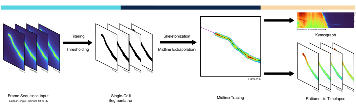
Figure 1: An overview of the pipeline workflow. The AMEBaS pipeline analyses and processes microscopic time lapses in three main steps: Single-Cell Segmentation, Midline Tracing, and Kymograph Generation. Please click here to view a larger version of this figure.

Protocol

1. Interactive notebook protocol

The Jupyter notebook can be used directly on the web using Google Colab at https://colab.research.google.com/github/badain/amebas/blob/main/AMEBAS_Colab.ipynb, where the instructions below were based. Alternatively, the Jupyter notebook is available at https://github.com/badain/amebas, where it can be downloaded and configured to run locally in Jupyter (Anaconda can provide an easy and cross-platform installation process). A complete test data can be found at Zenodo (https://doi.org/10.5281/zenodo.7975350), containing single and dual channel data of Arabidopsis pollen tubes expressing either pH or Ca​²⁺ reporters¹⁴. The pipeline has been divided into parts, where every step can be executed by clicking on the play button after setting the user-specific options. The necessary files for this study are available in AMEBaS- main zip folder (Supplementary Coding File 1).

1. Open Jupyter notebook and read the time-lapse files.
   1. Navigate to the homepage of the interactive notebook in Google Colab referred above or download and open the AMEBaS_Local.ipynb notebook from GitHub.
   2. Prepare the directory setup for the input and output data:
      1. If using the local version, place the fluorescence time-lapse as a TIFF file or DV file inside a folder named data that must be in the root folder of the program. A folder named out must be created to receive the generated data. Then run the Setup code block.
      2. If using the notebook on Google Colab, run the Setup code block to automatically generate the data and out folders.
   3. Run the File Input code block to read the time lapse data by clicking the play button. If using the Google Colab version of the notebook, click on the Choose File button to directly upload the time lapse file to the data folder.
      ​NOTE: The number of channels will be automatically detected based on the dimension of the image.
   4. Choose if additional outputs of each step will be generated by setting the 'verbose' parameter to True or False.
2. Detect the main cell and segment from the background (Figure 2).
   1. Run the Single Cell Segmentation code block to automatically separate the cell of interest from the background by clicking the play button.
      NOTE: Median and Gaussian filters will be applied as a preprocessing step to remove unwanted noise before segmenting the foreground from the background by Isodata thresholding and isolating the region of the largest area to remove undesired artifacts.
      1. Adjust the sigma value used by the Gaussian in the 'sigma' variable to fine-tune the smoothness of the segmentation mask. The default value is 2.0.
      2. Set the variable estimate to False to store the threshold estimated from Isodata directly or to True to smooth it across neighboring frames using local polynomial regression (LOESS). Fine-tune its function by changing the n_points variable. The default value is 40.
3. Trace midline along the cell extension (Figure 3).
   1. Run the Cell Midline Tracing code block by clicking the play button to automatically skeletonize the cell using Lee's method¹⁸ and extend the tip of the last skeleton through linear extrapolation.
      1. Choose to trace the midline only on the last frame or once per frame by adjusting the complete_skeletonization argument.
         NOTE: When all frames are skeletonized, extrapolation is skipped.
      2. Set the fraction of points in the skeleton to be interpolated during extrapolation by adjusting the interpolation_fraction variable. The default value is 0.25.
      3. Choose the length of the midline extrapolation by changing the variable extrapolation_length. The default is -1, which extends the skeleton up to the nearest edge.
4. Generate kymographs for each channel ( Figure 4).
   1. Run the first Data Visualization code block by clicking the play button to automatically generate kymographs for both channels.
      1. Choose the size of the Gaussian kernel used for smoothing by adjusting the variable kymograph_kernel.
         NOTE: It corresponds to the size of the neighborhood (in pixels) over which the pixel intensities are averaged. The default is 3 pixels x 3 pixels.
      2. Nonextended skeletons generate capped Kymographs that must use a custom colormap to properly display their intensities. Choose the fraction percentage of the intensities that will be assigned to the background color, black, adjusting the shift_fraction variable. The default value is 0.7.
5. Calculate the ratio between channels (Figure 5).
   1. Run the second Data Visualization code block by clicking the play button to automatically generate a ratiometric kymograph and a ratiometric timelapse (Figure 6).
      NOTE: This step is only available when using dual-channel time lapses. The background intensity threshold stored in step 1.2.1.2 is subtracted from each channel.
      1. Adjust the switch_ratio variable to switch the order of channels used as the numerator and denominator during ratio calculations. The default is False.
      2. Choose if the ratio timelapse must be further smoothed with a median filter pass by adjusting the smooth_ratio variable. The default is False.
      3. Choose whether to remove outliers produced by the low signal of the denominator channel by manipulating the reject_outliers variable. Defaults to True and defines outliers as values 1.5 times the interquartile range above the third quartile (where 75% of the values lie).
      4. Choose whether the background in the ratiometric output must be exported by adjusting the variable background_ratio. The default is False, which replaces it with zeros.

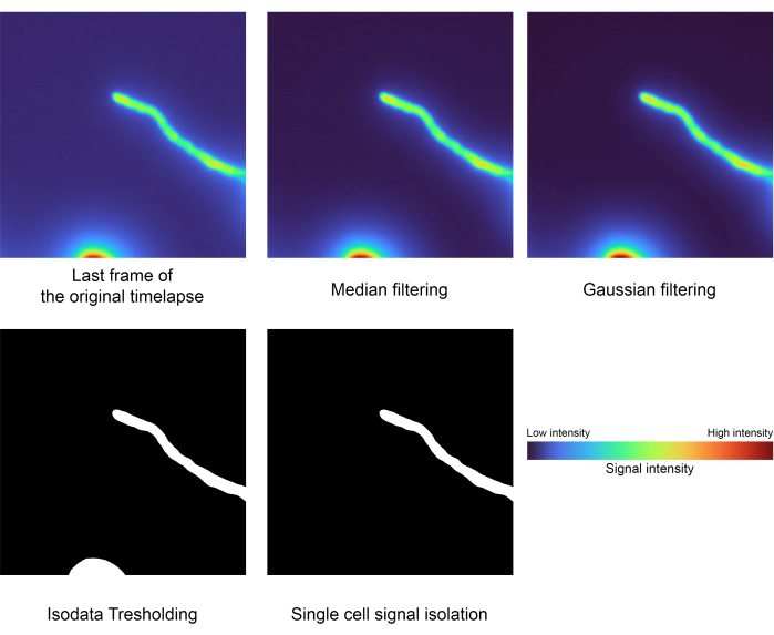
Figure 2: Single cell segmentation step. Image processing techniques such as filtering, thresholding, and area labeling are used to isolate the signal of interest (step 1.2). This particular data had the following values for Lowest Intensity: 2556, Median: 3441, and Highest Intensity: 32125. Please click here to view a larger version of this figure.

Figure 3: Midline tracing overview- The midline of the single cell is obtained by calculating its skeleton (white). The tip (magenta) is extrapolated linearly from the last points at the end of the skeleton (step 1.3). In this composition both the midline and its tip are superposed over the original cell. Please click here to view a larger version of this figure.

Figure 4: Timelapse's kymographs- Comparison of the kymographs for each channel generated with 'complete_skeletonization' turned off (step 1.4). The vertical axis describes the progression of time, and the horizontal axis plots the average intensity of the extrapolated midline path followed by a single cell. For this particular data, the colormap represents the following values for Channel 1 Lowest Intensity: 2886, Median: 3167, Highest Intensity: 21021. Channel 2 Lowest Intensity: 3030, Median: 3400, Highest Intensity: 29688. Please click here to view a larger version of this figure.

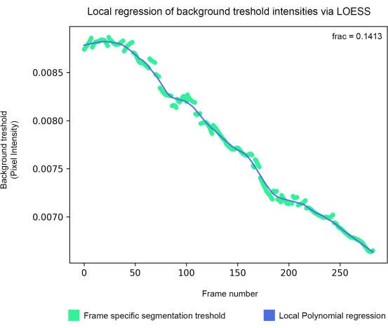
Figure 5: Background threshold smoothing- The background segmentation threshold is estimated via the isodata algorithm and then smoothed via local polynomial regression (step 1.5). Please click here to view a larger version of this figure.

Figure 6: Ratiometric results- (A) Comparison between the last frame of the ratiometric timelapse and the segmented original first channel. (B) Kymograph generated from the ratiometric timelapse (step 1.5). Please click here to view a larger version of this figure.

2. Batch mode protocol

1. Download and place the file pipeline.py from the AMEBaS GitHub repository in the same directory as the data.
2. Type in the file location on the command line after the program file.
3. Include --v as a positional argument to show the internal steps of the pipeline, if desired.
4. Include --s to choose in the sigma value used in the Gaussian Filter preprocessing step in preparation for cell segmentation. The default is 2.
5. Include --a to trace the midline for each frame of the time lapse. By default, the pipeline uses only the last frame.
6. Include --f to choose the fraction [0,1] of the skeleton to be used in the interpolation. The default value is 0.25.
7. Include -e to choose the length in pixels of the extrapolated skeleton. The default is -1, which extends the skeleton up to the nearest edge.
8. Include --sf to choose the fraction of the color range that will be shifted to the background in non-extrapolated kymographs. The default value is 0.7.
9. Include --k to determine the size of the kernel used in the kymograph Gaussian filtering. The default is 3.
10. Include --eb to estimate global background threshold intensity via LOESS polynomial regression of the frame-specific background threshold intensities.
    1. Customize the number of points used in LOESS smoothing of the background threshold values by modifying the parameter --n. The default value is 40.
11. Switch the channels used as the numerator and denominator during ratio calculations, including -r or --switch_ratio, if the timelapse has two channels. By default, the second channel is the numerator and the first is the denominator.
12. Choose if the ratio timelapse must be further smoothed with a Median Filter pass with the --sm argument. The default is False.
13. Include -o to reject pixels with abnormal intensities during ratiometric time-lapse generation.
14. Choose if the background in the ratiometric output must be exported using the argument --b. The default is False, which replaces it with zeros.
15. Press enter to run. The output will be generated in the same directory as the program file.

Results

The AMEBaS pipeline automates the extraction of midline dynamics of polarized single cells from fluorescence microscopy image stacks, making it less time consuming and less prone to human errors. The method quantifies these time lapses by generating kymographs and ratiometric image stacks (Figure 1) in growing single cells. It can be adjusted to work on migrating single cells, but further experiments are necessary. AMEBaS is implemented in Python as an interactive Jupyter Notebook (described...

Discussion

The novel method presented here is a potent tool to streamline and automate the analysis of fluorescence microscopy image stacks of polarized cells. Current methods described in the literature, such as ImageJ Kymograph plugins, require manual tracing of the midline of the polarized cell of interest, a task that is not only time consuming but also prone to human errors. Since the definition of the midline in this pipeline is supported by a numerical method^18,19 th...

Materials

List of materials used in this article

Name	Company	Catalog Number	Comments
Github	Github		https://github.com/badain/amebas
Google Colab	Google		https://colab.research.google.com/github/badain/amebas/blob/main/AMEBAS_Colab.ipynb

References

- Drubin, D. G., Nelson, W. J. Origins of cell polarity. Cell. 84 (3), 335-344 (1996).
- Wodarz, A., Näthke, I. Cell polarity in development and cancer. Nature Cell Biology. 9 (9), 1016-1024 (2007).
- Palanivelu, R., Preuss, D. Pollen tube targeting and axon guidance: parallels in tip growth mechanisms. Trends in Cell Biology. 10 (12), 517-524 (2000).
- Portes, M. T., et al. The Pollen Tube Oscillator: Integrating Biophysics and Biochemistry into Cellular Growth and Morphogenesis. Rhythms in Plants: Dynamic Responses in a Dynamic Environment. , Springer. Cham. (2015).
- Wudick, M. M., et al. CORNICHON sorting and regulation of GLR channels underlie pollen tube Ca2+ homeostasis. Science. 360 (6388), 533-536 (2018).
- Hoffmann, R. D., et al. Plasma membrane H+-ATPases sustain pollen tube growth and fertilization. Nature Communications. 11 (1), 1-15 (2020).
- Michard, E., et al. Glutamate receptor-like genes form Ca2+ channels in pollen tubes and are regulated by pistil D-serine. Science. 332 (6028), 434-437 (2011).
- Damineli, D. S., Portes, M. T., Feijó, J. A. Oscillatory signatures underlie growth regimes in Arabidopsis pollen tubes: computational methods to estimate tip location, periodicity, and synchronization in growing cells. Journal of Experimental Botany. 68 (12), 3267-3281 (2017).
- Li, K., et al. An optimized genetically encoded dual reporter for simultaneous ratio imaging of Ca2+ and H+ reveals new insights into ion signaling in plants. New Phytologist. 230 (6), 2292-2310 (2021).
- Sadoine, M., et al. Designs, applications, and limitations of genetically encoded fluorescent sensors to explore plant biology. Plant Physiology. 187 (2), 485-503 (2021).
- Grenzi, M., et al. Illuminating the hidden world of calcium ions in plants with a universe of indicators. Plant Physiology. 187 (2), 550-571 (2021).
- Munglani, G., Vogler, H., Grossniklaus, U. Fast and flexible processing of large FRET image stacks using the FRET-IBRA toolkit. PLoS Computational Biology. 18 (4), 1009242(2022).
- Ridler, T., Calvard, S. Picture thresholding using an iterative selection method. IEEE Transactions on Systems, Man, and Cybernetics. 8 (8), 630-632 (1978).
- Portes, M. T., Feijó, J. Growing Arabidopsis pollen tubes expressing genetically encoded reporters for calcium and pH. , (2023).
- Candeo, A., Doccula, F. G., Valentini, G., Bassi, A., Costa, A. Light sheet fluorescence microscopy quantifies calcium oscillations in root hairs of Arabidopsis thaliana. Plant & Cell Physiology. 58 (7), 1161-1172 (2017).
- Romano Armada, N., et al. In vivo light sheet fluorescence microscopy of calcium oscillations in Arabidopsis thaliana. Methods in Molecular Biology. 1925, 87-101 (2019).
- Krebs, M., et al. FRET-based genetically encoded sensors allow high-resolution live cell imaging of Ca2+ dynamics. The Plant Journal. 69 (1), 181-192 (2012).
- Lee, T. -C., Kashyap, R. L., Chu, C. -N. Building skeleton models via 3-D medial surface axis thinning algorithms. CVGIP: Graphical Models and Image Processing. 56 (6), 462-478 (1994).
- Nunez-Iglesias, J., Blanch, A. J., Looker, O., Dixon, M. W., Tilley, L. A new Python library to analyse skeleton images confirms malaria parasite remodelling of the red blood cell membrane skeleton. PeerJ. 6, 4312(2018).
Access restricted. Please log in or start a trial to view this content.
Reprints and Permissions