Measuring Local Tissue Strains in Tendons via Open-Source Digital Image Correlation

Summary

This paper describes an open-source digital image correlation algorithm for measuring local 2D tissue strains within tendon explants. The accuracy of the technique has been validated using multiple techniques, and it is available for public use.

Abstract

There is considerable scientific interest in understanding the strains that tendon cells experience in situ and how these strains influence tissue remodeling. Based on this interest, several analytical techniques have been developed to measure local tissue strains within tendon explants during loading. However, in several cases, the accuracy and sensitivity of these techniques have not been reported, and none of the algorithms are publicly available. This has made it difficult for the more widespread measurement of local tissue strains in tendon explants. Therefore, the objective of this paper was to create a validated analysis tool for measuring local tissue strains in tendon explants that is readily available and easy to use. Specifically, a publicly available augmented-Lagrangian digital image correlation (ALDIC) algorithm was adapted for measuring 2D strains by tracking the displacements of cell nuclei within mouse Achilles tendons under uniaxial tension. Additionally, the accuracy of the calculated strains was validated by analyzing digitally transformed images, as well as by comparing the strains with values determined from an independent technique (i.e., photobleached lines). Finally, a technique was incorporated into the algorithm to reconstruct the reference image using the calculated displacement field, which can be used to assess the accuracy of the algorithm in the absence of known strain values or a secondary measurement technique. The algorithm is capable of measuring strains up to 0.1 with an accuracy of 0.00015. The technique for comparing a reconstructed reference image with the actual reference image successfully identified samples that had erroneous data and indicated that, in samples with good data, approximately 85% of the displacement field was accurate. Finally, the strains measured in mouse Achilles tendons were consistent with the prior literature. Therefore, this algorithm is a highly useful and adaptable tool for accurately measuring local tissue strains in tendons.

Introduction

Tendons are mechanosensitive tissues that adapt and degenerate in response to mechanical loading^1,2,3,4. Due to the role that mechanical stimuli play in tendon cell biology, there is a large interest in understanding the strains that tendon cells experience in the native tissue environment during loading. Several experimental and analytical techniques have been developed to measure local tissue strains in tendons. These include 2D/3D digital image correlation (DIC) analyses of surface strains using either speckle patterns or photobleached lines (PBLs)^5,6,7,8, measurement of the changes in the centroid-to-centroid distance of individual nuclei within the tissue^9,10, and a recent full-field 3D DIC method that considers out-of-plane motion and 3D deformations¹¹. However, the accuracy and sensitivity of these techniques have been reported in only a few cases, and none of these techniques have been made publicly available, which makes the widespread adoption and utilization of these techniques difficult.

The objective of this work was to create a validated analysis tool for measuring local tissue strains in tendon explants that is readily available and easy to use. The chosen method is based on a publicly available augmented-Lagrangian digital image correlation (ALDIC) algorithm written in MATLAB that was developed by Yang and Bhattacharya¹². This algorithm was adapted for analyzing tendon samples and validated by applying it to digitally transformed images and by comparing the strains measured in actual tendon samples to the results obtained from photobleached lines. Furthermore, additional functionality was implemented in the algorithm to confirm the accuracy of the calculated displacement field even in the absence of known strain values or a secondary measurement technique. Therefore, this algorithm is a highly useful and adaptable tool for accurately measuring local 2D tissue strains in tendons.

Protocol

This study was approved by the Pennsylvania State University Institutional Animal Care and Use Committee.

1. Tissue preparation

1. For this protocol, harvest the Achilles tendons from 2-4 month old male C57BL/6 mice.
   NOTE: Different tendons or ligaments from mice or other small animals could also be used.
   1. Make an incision to the skin superficial to the Achilles tendon to expose the plantaris tendon and the surrounding connective tissue. Then, remove them using a surgical blade.
   2. Separate the exposed soleus and gastrocnemius muscles from the hind limb, and carefully scrape them off the Achilles tendon with the surgical blade
   3. Separate the calcaneus from the rest of the foot with a cutting wheel attachment on a rotary tool.
2. Stain the tissue in 1.5 mL of a 5 µg/mL solution of 5-(4,6-dichlorotriazinyl) aminofluorescein (DTAF) and 0.1 M sodium bicarbonate buffer for 20 min on a rotating mixer at room temperature. This solution stains proteins (e.g., extracellular matrix) in the tissue.
   NOTE: During this 20 min period, step 1.3 should be completed.
3. Prepare a 1:1,000 solution of DRAQ5 in phosphate-buffered saline (PBS) to stain the nuclei. Use a vortex mixer to homogenize the solution.
4. After the 20 min incubation period in step 1.2, transfer the tissue from the DTAF solution to the DRAQ5 solution, and incubate in a dark space for 10 min at room temperature.

2. Tendon loading and image acquisition

NOTE: This protocol requires a tensile device that can be mounted on top of a confocal microscope. For this study, the microtensile device described by Peterson and Szczesny¹³ was used.

1. Place the tendon into the grips of the tensile loading device. Prior to mounting the grips in the loading device, use digital calipers to measure the distance between the calcaneus attachment and the opposite grip. This distance is the tendon gauge length.
   1. Alternatively, mount the grips into the loading device prior to inserting the tendon, and push into contact to define the zero-displacement motor position. The displacement of the motors after inserting the tendon could provide a potentially more accurate grip-to-grip gauge length.
2. Mount the grips into the loading device, which contains PBS to maintain tissue hydration. Align the tendon as best as possible with either the x-axis or y-axis of the microscope images so that the x-strain and y-strain outputs of the algorithm correspond with the tendon axes.
   ​NOTE: In this study, the tendons were aligned with the x-axis. If it is not possible to perfectly align the tendon with the image axes, then the x-strain and y-strain outputs of the algorithm can be transformed to align with the longitudinal/perpendicular axes of the tendon using standard strain transformation equations¹⁴.
3. Preload the tendon with 1 g of tension, and, if desired, apply cyclic loading to precondition the sample. In this protocol, no preconditioning was used since the study objective was to validate the measured local tissue strains rather than measure the tissue material properties. If there is interest in measuring the macroscale material properties, which are dependent on the loading history, then preconditioning is recommended. Following preconditioning and recovery, reapply a 1 g preload.
4. If desired, photobleach a set of four lines spaced 80 µm apart in the center region of the tissue (see Peterson and Szczesny¹³ for more details).
   NOTE: The photobleached lines were used to validate the measurements of the ALDIC algorithm and are not necessary for performing the ALDIC itself. The number and spacing of the lines can be adjusted, and the location of the lines should be chosen to avoid any artifacts in the sample that would decrease the clarity of the line.
5. Repeat the photobleaching procedure on the left and right extremes of the tissue near the grips.
6. Using the confocal microscope, acquire volumetric images (x,y: 1.25 µm/pixel, z: 2.5 µm/pixel) of the DTAF and DRAQ5 fluorescence at 1 g of preload.
7. Perform a strain ramp at 0.5%/s to 2% strain. Note that the strain rate and incremental strain magnitude can be adjusted.
8. Allow the tissue to stress relax for 10 min.
   NOTE: The duration of stress relaxation should be chosen such that the sample is under an approximately quasistatic load during image acquisition. To determine if the stress relaxation duration is acceptable, determine the slope of the force-time curve during the final minute of stress relaxation (Supplementary Figure 1), and multiply this slope by the total imaging duration. In this study, the force applied at the largest strain increment never changed by more than 5%.
9. Take another volumetric image of the tissue after deformation.
10. Repeat steps 2.7-2.9 until the desired final strain is reached. In this paper, a final strain value of 12% was chosen.

3. Image processing

1. Use ImageJ or Fiji to create maximum z-projections of each volumetric image of the DRAQ5 (nuclear) channel. This will serve as the 2D speckled images for the ALDIC.
2. Save the max-intensity z-projections as .tiff files, and name them according to the following naming convention.
   1. Use a number as the first character of the image name.
   2. Have the number correspond to the order in which the images will be considered during the strain analysis. For example, the first image should begin with one, and the second image should begin with two. Different numbers can be chosen, but they must sequentially increase. An example naming convention is as follows: "0_Experiment1_MaxZProjection".
3. Save all the renamed max-intensity z-projections to a folder.

4. Photobleached line analysis code installation and application

NOTE: These steps are only necessary if it is desired to confirm the accuracy of the ALDIC algorithm using photobleached lines. The code calculates the local tissue strain as the average normalized change in distance between each photobleached line within the photobleached line set. In this study, the average local values were then averaged across all the photobleached line sets (i.e., at the center and the left/right ends) to determine a single average local tissue strain value for each sample. This value was then used to estimate the accuracy of the ALDIC algorithm.

1. Download the "PBL Code" folder from GitHub (https://github.com/Szczesnytendon/TendonStrainCalc), and move all the contents to the working directory in MATLAB.
2. Open the "Micro_Mech_Template.m" MATLAB script.
   1. Press Run, and select one of the image files containing the volumetric images. The volumetric images can be any of the following file types: .lsm, .tiff, .nd2.
   2. The software will automatically load all the images in the folder and display a projected image of the reference volumetric image. When prompted, left-click to create multi-point lines that trace the left and right ends of the sample. Right-click to terminate a line. Once the input has been processed, if the edges are correct, press Ok to accept the result.
   3. Draw a random diagonal line across the sample as a reference line when prompted.
   4. Input the number of photobleached lines created, and trace the photobleached lines with multi-point lines.
   5. If the result is acceptable, accept it. If the result is erroneous, adjust it and reprocess.
3. Repeat step 4.2 for all the images, and move all the images of traced lines into a single folder.
4. Open the script "Micro_Mech_Strain.m".
   1. Press Run to execute the code, and select one of the saved images where the photobleached lines are traced.
   2. Confirm that the selected accompanying images are correct once the image is selected by pressing Ok.

5. Creating digitally transformed images

NOTE: These steps are only necessary if it is desired to confirm the accuracy of the ALDIC algorithm using digitally transformed images. These images simulate homogenous 2D strain fields of a known magnitude by artificially transforming the reference image.

1. Download the code "Digital_strain.m" from GitHub (https://github.com/Szczesnytendon/TendonStrainCalc).
2. Open and run the code.
3. When prompted, insert desired values for the maximum applied strain, applied strain increment, and Poisson's ratio. Press Ok.
   NOTE: For this experiment, the maximum applied strain was 0.1 (10%), the applied strain increment was 0.02 (2%), and a Poisson's ratio of 1 was used, which is consistent with experimental data of tendon tensile testing^15,16. The code uses the embedded MATLAB function imwarp and the input values (e.g., strain increments, Poisson's ratio) to create the digitally transformed images.
4. When prompted, select the undeformed reference image.
5. For each strain increment, an overlay of the reference image and the transformed image is displayed. The transformed image will be saved to the directory under the title "DigitallyTransformedX%Strain", where X is the strain increment.

6. Strain calculation and validation code installation and application

1. Download the "Strain Calculation and Validation Code" folder from GitHub (https://github.com/Szczesnytendon/TendonStrainCalc), and move all the contents to the MATLAB working directory
2. Install a mex C/C++ compiler according to Yang and Bhattacharya¹². The steps are summarized below.
   1. Check MATLAB to see if a mex C/C++ compiler has been installed by typing "mex -setup" in the MATLAB Command Window and pressing Enter.
   2. If an error appears indicating that a compiler is not supported or present, proceed to step 6.3 and step 6.4.
   3. If no error is present, proceed to step 6.5
3. To download a mex C/C++ compiler, go to "https:/tdm-gcc.tdragon.net/", and choose the TDM-gcc compiler.
4. Install the downloaded compiler to a known location.
5. Return to the MATLAB command window, and type: "setenv("MW_MINGW64_LOC","[Type your install path here]")". For example, this could be "setenv("MW_MINGW64_LOC","C:\TDM-GCC-64")". If this command executes successfully, the mex compiler is properly installed.
6. Enter the "main_aldic.m" function script, and change line 22 to match the command executed in step 6.5.
7. Open the script "Strain_calc_and_validate.m".
8. Press Run to begin the image analysis.
9. When prompted, alter the values for the ALDIC parameters as desired.
   NOTE: The window size should be 0.25 to 1 times the subset size. For more information about the parameter choices, refer to the online user manual: (https://www.researchgate.net/publication/344796296_Augmented_Lagrangian_Digital
   _Image_Correlation_AL-DIC_Code_Manual). 
   1. The following values were used in this study:
      Subset Size (pixels): 20
      Window Size (pixels): 10
      Method to solve ALDIC: Finite Difference (1)
      Parallel computing was not used (1)
      Method to compute initial guess: Multigrid search based on image pyramid (0)
10. When prompted, select the "Yes" checkbox to have the algorithm automatically save the mean value, standard deviation, and 2D maps for the desired collection of variables (e.g., x-strain, y-strain, shear strain, bad regions, etc.). Select which variables should be saved, and press Ok.
11. When prompted, alter the parameters as desired.
    1. The following values were used in this experiment:
       Surrounding points to calculate strain (numP): 12
       Correlation coefficient for bad region identification (corr_threshold): 0.5
       Subregion size (pixels) for bad region analysis (Subsize): 32
12. When prompted, select the folder that contains the renamed max-intensity z-projections. Note that the software automatically performs incremental ALDIC to determine the strain fields of the deformed images. That is, each deformed image serves as the new "reference" image for the next deformed image. This improves the accuracy of the results (Supplementary Figure 2) compared to performing cumulative ALDIC, where each deformed image is compared back to the original (0% strain) reference image. To perform a cumulative analysis, load the images but only select the original reference image and the deformed image of interest.
    NOTE: The normal strain is calculated as λ - 1, where λ is the tissue stretch. The tissue stretch is calculated according to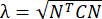 , where N = [1 0]^T or [0 1]^T for the x-direction and y-direction, respectively, and C = F^T F, where F is the deformation gradient calculated using "numP" points surrounding each data point output by the ALDIC algorithm. The shear strain is calculated as , where .
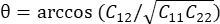13. When prompted, left-click to create a four-point polygon to define the region of interest for measuring the strains. Begin with the point in the top-left corner, and assign the subsequent points in a clockwise manner.
    NOTE: The variable "Storage" saved in the MATLAB workspace contains all the values for the average x-strain, x-strain standard deviation, average y-strain, y-strain standard deviation, average shear strain, shear strain standard deviation, and percentage of bad regions. The bad regions are defined according to the correlation coefficient analysis within the region of interest selected in step 6.13. The folder "NuclearTrackingResults" (which can be renamed by adjusting lines 555 and 556) stores all the plots specified in step 6.10. This folder also contains a spreadsheet file with the name "Results", which stores all the means and standard deviations specified in step 6.10.

Representative Results

Prior to analyzing the strain fields in actual tissue samples, the ALDIC protocol was first validated using digitally strained/transformed images of nuclei within mouse Achilles tendons. Specifically, the images were transformed to digitally produce uniform strains in the x-direction of 2%, 4%, 6%, 8%, and 10% strain with a simulated Poisson's ratio of 1^15,16. The accuracy of the ALDIC algorithm was then assessed by comparing the mean calculated strain values with the known digital strains. Additionally, the standard deviation of the strain values was assessed to determine the heterogeneity of the strain field. The difference between the strains calculated by ALDIC (using incremental analysis) and the actual strains applied to the digitally transformed images are shown in Figure 1. The mean strain in the x-direction calculated by the ALDIC software was consistently an underestimate of the true applied strain (Figure 1A), and the magnitude of the error increased with greater applied strain. However, the magnitude was always less than 0.00015 for all the strain increments. There was a slight underestimation of the strain in the y-direction as well (Figure 1C). The standard deviation of the calculated strains within the full region of interest for the x-strain and y-strain also increased with greater applied strains, but the magnitude was also very small (<0.002) (Figure 1B, D). These errors were substantially larger when using cumulative analysis (Supplementary Figure 2).

Figure 1: Algorithm comparison and validation with digitally strained images. (A) The measured ALDIC strain data in the x-direction was consistently lower than the actual strain prescribed by the digital transformations, and the error progressively increased with greater applied strain. (B) The standard deviation of the strain values in the x-direction also increased with greater applied digital strains. (C) The measured ALDIC strain data in the y-direction were consistently lower than the actual strain prescribed by the digital transformations. (D) The standard deviation of the strain values in the y-direction increased with greater applied strain. Please click here to view a larger version of this figure.

When performing strain analysis on actual tissue samples, it is not possible to directly assess the accuracy of the ALDIC algorithm. Still, a technique was developed to estimate the accuracy of the displacement field. Specifically, the deformed image was warped back into a prediction of the reference image based on the calculated displacement field. A normalized cross-correlation coefficient was then used to determine how well the warped/reconstructed reference image matched the true reference image. Any subregions (32 pixels x 32 pixels) in which the normalized cross-correlation value was less than 0.5 were considered a "bad region" in which the displacement field was likely inaccurate. This analysis identified that there was a significant difference between the performance of the incremental and cumulative analysis techniques. Specifically, the number of bad regions began to rise with the cumulative method after the 6% applied strain (Figure 2A), whereas very few (1%) bad regions were observed in any of the digitally transformed regions for the incremental analysis. When applying this accuracy assessment technique on the four mouse Achilles tendons that were tested (Supplementary Figure 3), it was determined that for three samples, the average number of bad regions was less than 25% of the image. However, in one of the four samples (Experiment 2), nearly half of the image was identified as bad at the maximum strain increment (Figure 2B). The number of bad regions that were present in Experiment 2 varied from the mean of the other three samples by over four standard deviations. This enabled the determination that the ALDIC data from Experiment 2 represented an outlier, and these data were, therefore, eliminated from the further analysis of the results.

Figure 2: Successful identification of areas with invalid strain calculations by bad region analysis. (A) The quantity of bad regions in the digitally transformed images analyzed using the cumulative method increased consistently after 6% applied strain, while the incremental quantity remained at 1%. (B) The quantity of bad regions for all the tendon samples increased steadily at larger strain increments. Experiment 2 was considered an outlier and, thus, is not included in the mean and standard deviation bars. Please click here to view a larger version of this figure.

Additionally, the local tensile strains in the tested mouse Achilles tendons were measured using photobleached lines (PBLs) as a second method for determining the accuracy of the ALDIC algorithm. The x-direction strains calculated by ALDIC tended to be larger than those determined from the PBLs, but the difference was generally within 0.005 strain (Figure 3A). This error magnitude was similar to the standard deviation observed across the different PBLs within a given sample (Figure 3B).

Figure 3: Validation of the ALDIC strain calculations by comparison with photobleached line data. (A) The difference between the ALDIC strain values and the PBL strain values remained relatively constant for all the strain increments, around a value of 0.005. (B) The standard deviation for the PBL data averaged across all the samples remained relatively constant at approximately 0.005. Please click here to view a larger version of this figure.

After assessing the accuracy of the ALDIC algorithm, the magnitudes and spatial distributions of the local strains in the mouse Achilles tendons under tensile load were determined (Figure 4, Figure 5, and Figure 6). Note that the strains do not include the displacement data from the "bad regions" within each sample. The x-direction tensile strains were consistent across all three samples and were substantially lower than the applied tissue strains (Figure 4A). Additionally, the x-direction strain was relatively heterogeneous, given that the standard deviation across the 2D image was always larger than the average strain value. In contrast, there was significant inconsistency between the three samples for the y-direction strains, with one sample exhibiting positive mean values, one sample exhibiting negative mean values, and one sample exhibiting zero strain in the y-direction (Figure 4B). Additionally, the standard deviation of the y-direction strains within a given sample was larger than the standard deviation of the x-direction strains. Finally, the shear strain was relatively low across all the strain increments (Figure 4C).

Figure 4: Microscale strains of mouse Achilles tendons. (A) The mean strain in the x-direction remained below the applied tissue strain but increased with each strain increment. (B) The mean strain in the y-direction was approximately zero for all the increments, but the standard deviation was high. (C) The mean shear strain increased steadily throughout the strain increments. Please click here to view a larger version of this figure.

Figure 5: Spatial distribution of x-strains, y-strains, and shear strains. Representative maps of the (A) x-strains, (B) y-strains, and (C) shear strains throughout the tendon region of interest Please click here to view a larger version of this figure.

Figure 6: Spatial distributions of maximum principal, minimum principal, and maximum shear strains. Representative maps of the (A) maximum principal strains, (B) minimum principal strains, and (C) maximum shear strains throughout the tendon region of interest. The white lines indicate the directions of the maximum and minimum principal stresses. Please click here to view a larger version of this figure.

Supplementary Figure 1: Identification of quasistatic state during imaging. The slope of the force-time curve during the final minute of the stress relaxation period (red line) can be used to approximate the overall change in force during imaging. Please click here to download this File.

Supplementary Figure 2: Comparison of incremental and cumulative analysis techniques. (A) The difference between the measured and actual x-direction strains in the digitally transformed images was significantly greater with the cumulative method as compared with the incremental method above 4% strain. (B) The standard deviation of x-strain values was also significantly greater with the cumulative method above 4% strain. (C) The difference between the measured and actual y-strains in the digitally transformed images was substantially larger with the cumulative method above 8% strain. (D) The standard deviation of the y-strain values was significantly greater with the cumulative method above 4% strain. Please click here to download this File.

Supplementary Figure 3: Bad region visualization and quantification for each experiment. Bad regions were defined as local areas within the reconstructed reference image that did not match (below correlation coefficient of 0.5) the same region of the actual reference image. Each bad region identified within a region of interest (outlined in white) is marked by a blue box. The percentage of bad regions within the region of interest is indicated above each image in parentheses. Note that these images are reconstructed from the deformed image at 12% applied strain. Please click here to download this File.

Discussion

The objective of this paper was to provide an open-source, validated method to measure the 2D strain fields in tendons under tensile load. The foundation of the software was based on a publicly available ALDIC algorithm¹². This algorithm was embedded into a larger MATLAB code with the added functionality of incremental (versus cumulative) strain analysis. This adapted algorithm was then applied to the tensile testing of tendons, and its accuracy was assessed by two different techniques (i.e., digitally transformed images and strain measurement using photobleached lines). Additionally, an ability was added to assess the accuracy of the ALDIC measurements on any sample without requiring knowledge of the true strain values.

The analysis of the digitally transformed images demonstrated that the algorithm could accurately measure strains up to 10% with very little error, which could not be assessed from the tensile testing of actual mouse Achilles tendons due to the low magnitudes of the strains in the tendon samples. Nevertheless, comparing the strains calculated in mouse Achilles tendons by ALDIC to the strains measured using photobleached lines demonstrated that the error of the ALDIC technique was within the measurement variation of the photobleached lines themselves. As a final validation, the accuracy of the full 2D displacement fields calculated by the ALDIC algorithm was assessed by reconstructing the reference image from the deformed image and comparing the reconstruction to the actual reference image. In the digitally transformed images, there was an increase in the number of bad regions and strain error with greater applied strains, especially for the cumulative ALDIC analysis (Figure 2 and Supplementary Figure 2). This was expected since the incremental technique redefines the reference image with each intermediate image to minimize the displacement differences between image pairs. The number of bad regions was even higher in the actual tendon samples since the structure and loading of the tendon tissue were not homogenous (unlike the digitally transformed images). Still, on average, only about 15% of the reconstructed image did not match the actual reference image. However, one sample (Experiment 2) did have a large number of erroneous regions (~45%). While it is unclear why this sample could not be properly processed, this analysis of the reconstructed reference image was valuable because it enabled the recognition that the data from this sample were not reliable. Altogether, these experiments demonstrate that this open-source algorithm can be confidently used to accurately measure tissue strains within tendon explants.

These experiments also provided valuable information regarding the mechanical behavior of mouse Achilles tendons. Specifically, at an applied tissue strain of 12%, the average longitudinal (x-direction) strain within the tissue sample was only 2%. Part of this strain attenuation was due to the fact that the macroscale tissue strains were calculated from changes in the grip-to-grip length of the tissue, which likely included significant strain concentrations at the grip interface of the myotendinous junction. Still, this is consistent with other studies of microscale strains in tendons^10,17,18. Furthermore, the 12% strain corresponded to approximately 5 MPa of loading, which is likely comparable to the maximum physiological loads in vivo¹⁹. This suggests that cells within mouse Achilles tendons do not experience tensile strains above 2%. The transverse (y-direction) strain was more variable across samples, with both positive and negative values. This suggests that the tendon samples exhibited positive and negative Poisson's ratios, which is consistent with prior testing of Achilles tendons²⁰. As expected for uniaxial tension, the magnitude of the shear strain was generally low (<4° on average). However, for all the tensile and shear strains, the standard deviation across the region of interest was always greater than the average strain value, demonstrating that there was a large degree of strain heterogeneity. Furthermore, this heterogeneity increased with greater applied strains, likely due to the heterogeneity of the tissue structure as well as the increased error within the ALDIC calculations resulting from the larger displacements and displacement fields. This suggests that the strains experienced by individual tendon cells are highly variable within the tissue.

Despite the successful validation of the ALDIC algorithm, there are some limitations in its use for analyzing strains within tendon explants. The primary limitation is the fact that the algorithm can only perform a 2D analysis of a 3D object. A more rigorous approach would be to perform a full digital volume correlation (DVC), which has been performed on digitally transformed images of tendons¹¹. However, this is generally difficult to perform on actual tendon samples since the images contain resolvable nuclei to a depth of only 100 µm. This means that the interior volume of the samples has no texture within the volumetric images, making the DVC unreliable. Therefore, the images in this study were collapsed to 2D maximum projections, which artificially forces all the nuclei into a single image plane. While this may produce some errors in the strain analysis and prevent the measurement of out-of-plane displacements, the validation results suggest that the technique is still accurate. An additional limitation is that the strains were calculated at the end of a stress relaxation period and could not be calculated during dynamic cyclic loading. This issue was unavoidable since there was a finite imaging time to acquire the volumetric images used for the strain analysis. Despite these limitations, the success of the analysis was relatively robust, given that three out of the four tendon samples produced accurate strain data. Therefore, this algorithm will be a useful tool for researchers interested in measuring strain fields within tendon explants.

Materials

Name	Company	Catalog Number	Comments
5-DTAF (5-(4,6-Dichlorotriazinyl) Aminofluorescein), single isomer	ThermoFisher	D16
Calipers	Mitutoyo	500-196-30
Confocal Microscope	Nikon	A1R HD
Corning LSE Vortex Mixer	Coning	6775
DRAQ5 Fluorescent Probe Solution (5 mM)	ThermoFisher	62554
MATLAB	MathWorks	R2022b
Tensile Loading Device	N/A	N/A	Tensile loading device described in Peterson et al, 2020. (ref 13)
Tube Revolver Rotator	ThermoFisher	88881001

References

- Devkota, A. C. Distributing a fixed amount of cyclic loading to tendon explants over longer periods induces greater cellular and mechanical responses. Journal of Orthopaedic Research. 11 (4), 1609-1612 (2007).
- Sun, H. B., et al. Cycle-dependent matrix remodeling gene expression response in fatigue-loaded rat patellar tendons. Journal of Orthopaedic Research. 28 (10), 1380-1386 (2010).
- Shepherd, J. H., Screen, H. R. C. Fatigue loading of tendon. International Journal of Experimental Pathology. 94 (4), 260-270 (2013).
- Paschall, L., Pedaprolu, K., Carrozzi, S., Dhawan, A., Szczesny, S. Mechanical stimulation as both the cause and the cure of tendon and ligament injuries. Regenerative Rehabilitation: From Basic Science to the Clinic. , Springer. Cham, Switzerland. 359-386 (2022).
- Andarawis-Puri, N., Ricchetti, E. T., Soslowsky, L. J. Rotator cuff tendon strain correlates with tear propagation. Journal of Biomechanics. 42 (2), 158-163 (2009).
- Cheng, V. W. T., Screen, H. R. C. The micro-structural strain response of tendon. Journal of Materials Science. 42 (21), 8957-8965 (2007).
- Luyckx, T., et al. Digital image correlation as a tool for three-dimensional strain analysis in human tendon tissue. Journal of Experimental Orthopaedics. 1 (1), 7 (2014).
- Duncan, N. A., Bruehlmann, S. B., Hunter, C. J., Shao, X., Kelly, E. J. In situ cell-matrix mechanics in tendon fascicles and seeded collagen gels: Implications for the multiscale design of biomaterials. Computer Methods in Biomechanics and Biomedical Engineering. 17 (1), 39-47 (2014).
- Arnoczky, S. P., Lavagnino, M., Whallon, J. H., Hoonjan, A. In situ cell nucleus deformation in tendons under tensile load; A morphological analysis using confocal laser microscopy. Journal of Orthopaedic Research. 20 (1), 29-35 (2002).
- Screen, H. R. C., Bader, D. L., Lee, D. A., Shelton, J. C. Local strain measurement within tendon. Strain. 40 (4), 157-163 (2004).
- Fung, A. K., Paredes, J. J., Andarawis-Puri, N. Novel image analysis methods for quantification of in situ 3-D tendon cell and matrix strain. Journal of Biomechanics. 67, 184-189 (2018).
- Yang, J., Bhattacharya, K. Augmented Lagrangian digital image correlation. Experimental Mechanics. 59 (2), 187-205 (2019).
- Peterson, B. E., Szczesny, S. E. Dependence of tendon multiscale mechanics on sample gauge length is consistent with discontinuous collagen fibrils. Acta Biomaterialia. 117, 302-309 (2020).
- Humphrey, J. D., O'Rourke, S. L. An Introduction to Biomechanics. , Springer. New York, NY. (2015).
- Reese, S. P., Weiss, J. A. Tendon fascicles exhibit a linear correlation between Poisson's ratio and force during uniaxial stress relaxation. Journal of Biomechanical Engineering. 135 (3), 34501 (2013).
- Ahmadzadeh, H., Freedman, B. R., Connizzo, B. K., Soslowsky, L. J., Shenoy, V. B. Micromechanical poroelastic finite element and shear-lag models of tendon predict large strain dependent Poisson's ratios and fluid expulsion under tensile loading. Acta Biomaterialia. 22, 83-91 (2015).
- Szczesny, S. E., Elliott, D. M. Interfibrillar shear stress is the loading mechanism of collagen fibrils in tendon. Acta Biomaterialia. 10 (6), 2582-2590 (2014).
- Han, W. M., et al. Macro- to microscale strain transfer in fibrous tissues is heterogeneous and tissue-specific. Biophysical Journal. 105 (3), 807-817 (2013).
- Pedaprolu, K., Szczesny, S. E. A novel, open-source, low-cost bioreactor for load-controlled cyclic loading of tendon explants. Journal of Biomechanical Engineering. 144 (8), 084505 (2022).
- Gatt, R., et al. Negative Poisson's ratios in tendons: An unexpected mechanical response. Acta Biomaterialia. 24, 201-208 (2015).