Real-Time Imaging of Bonding in 3D-Printed Layers

Summary

With a non-invasive and real-time technique, nanoscopic polymer motion inside a polymer filament is imaged during 3D printing. Fine-tuning this motion is crucial for producing constructs with optimal performance and appearance. This method reaches the core of plastic layer fusion, thus offering insights into optimal printing conditions and material design criteria.

Abstract

In recent times, 3D printing technology has revolutionized our ability to design and produce products, but optimizing the print quality can be challenging. The process of extrusion 3D printing involves pressuring molten material through a thin nozzle and depositing it onto previously extruded material. This method relies on bonding between the consecutive layers to create a strong and visually appealing final product. This is no easy task, as many parameters, such as the nozzle temperature, layer thickness, and printing speed, must be fine-tuned to achieve optimal results. In this study, a method for visualizing the polymer dynamics during extrusion is presented, giving insight into the layer bonding process. Using laser speckle imaging, the plastic flow and fusion can be resolved non-invasively, internally, and with high spatiotemporal resolution. This measurement, which is easy to perform, provides an in-depth understanding of the underlying mechanics influencing the final print quality. This methodology was tested with a range of cooling fan speeds, and the results showed increased polymer motion with lower fan speeds and, thus, explained the poor printing quality when the cooling fan was turned off. These findings show that this methodology allows for optimizing the printing settings and understanding the material behavior. This information can be used for the development and testing of novel printing materials or advanced slicing procedures. With this approach, a deeper understanding of extrusion can be built to take 3D printing to the next level.

Introduction

The method of 3D printing is an additive manufacturing technique in which an object is manufactured layer by layer to form the desired shape. This method has a large and diverse user-base thanks to its versatility, affordability, and ease of use. Fused deposition modeling features a moving extruder (with a diameter of hundreds of microns to a couple of millimeters) to deposit molten plastic into the desired shape¹. The extruded plastic should behave in a liquid-like manner for a certain duration to achieve good fusion with the previously printed plastic and form a strongly cohesive material. However, the plastic should cool down and solidify quickly after printing to prevent the plastic from flowing away from the print location and reducing the print quality. This delicate interplay between heating and cooling has been shown to directly underpin the balance between the mechanical strength and the geometric accuracy of the final 3D-printed object². To achieve the optimal heating-cooling balance, the plastic is extruded at a temperature just above its melting temperature, and a fan head, attached to the printer, is used to cool the plastic down quickly. An in-depth understanding of the effects of printing temperatures and cooling speeds could provide the insights required for developing advanced slicing and printing protocols that maximize the mechanical or geometric results in the areas where they are most important. Efforts to gain more insight into these processes often rely on infrared (IR) imaging, which only visualizes the surface temperature^3,4,5 and does not indicate the inner temperature of the plastic. Local heating beyond the melting transition drastically increases the polymer mobility and, thus, allows polymer entanglement between the old and new material. This temporally enhanced polymer motion is a requirement for the formation of the final cohesive material^6,7, but IR imaging can only measure polymer motion indirectly through the surface temperature^8,9. Translating the surface temperature to layer bonding thus necessitates precise knowledge of the core-surface temperature gradient and the associated complex polymer dynamics over a range of time and length scales. A direct measurement of the layer bonding (i.e., the polymer entanglement process) would allow the visualization of the mechanism underlying bulk material cohesion without a priori information or assumptions.

To gain an understanding of the spatial and temporal distribution of layer bonding, an imaging technique that directly quantifies the dynamics of the polymers that make up the plastic filament is employed in this work. This technique, laser speckle imaging (LSI), relies on interferometric light scattering to visualize nanoscopic motions, independent of the chemical composition. Depending on the optical properties of the sample, it can accurately measure several millimeters to centimeters into non-transparent materials^10,11,12, unlike IR imaging, which reports only surface temperatures^8,9. These attributes have recently made speckle-based methods popular in understanding dynamic processes in a plethora of materials, although they were originally developed for medical applications^10,11,12. Recently, LSI has been used to gain insight into the behavior of advanced polymeric materials such as self-cleaning liquid crystal polymer networks^13,14, as well as for predicting fracture in rubber¹⁵ and for studying self-healing materials¹⁶.

The feasibility of applying LSI to 3D printing was showcased in a previous article¹⁷, where a portable LSI setup with real-time analysis capabilities was presented, and it was shown that the deposition of molten plastic results in increased polymer motion multiple layers below the current layer. In the paper presented here, systematic research into the effects of the cooling fan speed on the degree of multi-layer bonding is performed. An improved plug-and-play version of the portable instrument is used that can be operated by users without optics or programming expertise. The speckle images are analyzed in real-time using Fourier transforms¹⁷, which visualize the amplitude of the speckle intensity fluctuations. This instrument has an additional brightfield camera that is aligned with the speckle camera so that the LSI motion maps can be overlayed with the brightfield images for easier interpretation without the brightfield light affecting the motion maps. The experimental approach presented in this article can be used to gain more insight into the melting, layer bonding, and solidification of extruded plastic during the 3D printing of challenging geometries and materials.

Protocol

1. Setup and alignment of the LSI instrument with the 3D printer

1. Place the 3D printer on a steady surface to minimize vibrations. Place the LSI instrument next to it so that the camera has a clear view of the printing area. Position the LSI instrument slightly higher than the 3D printer's build plate, and tilt it downward very slightly so that the view is not obstructed.
2. Turn on the laser and brightfield illumination, and verify that they are aligned with the imaging area. Set the laser power to 20 mW, ensure the laser exits the setup box expanded over a large area (multiple square centimeters), and ensure the power density is low enough (several times lower than a laser pointer) to be used in situ without additional safety measures like laser goggles or a black enclosures.
   CAUTION: Do not look directly into the laser.
3. Start with a test print (e.g., Supplementary Coding File 1 or Supplementary Coding File 2) to make the alignment and experimental setup more convenient (steps 1.3-1.6). Ensure that the LSI camera is focused on the printing area.
4. During this first test print, optimally align the lighting and digital camera. Adjust the laser direction so that the whole imaging area is illuminated homogeneously, and adjust the diaphragm such that the speckle size is slightly larger than the pixel size.
5. Optimize the framerate and exposure time such that the number of under-exposed and over-exposed pixels is minimized to achieve the maximum dynamic range.
6. Choose the right parameters for the live LSI data analysis; most importantly, select the frequency that produces the best imaging contrast between molten and solidified plastic. Adjust the region of interest (ROI) and colormap scaling. In this case, a Fourier series length of 16 was chosen, and the amplitude of the second frequency was visualized. As the speckle image collection rate is 50 frames per second, the visualized frequency is 6.25 Hz.
7. Prepare the LSI instrument to capture the images for one 3D printing experiment. Choose how often and for how long the images are saved. In this case, the images were saved every 0.25 s so that multiple images were saved per pass of the printer head. For each experiment, the images were saved for 15 min as each print job took a maximum of 12 min.

2. Preparation of the 3D-printing design and G-code

1. Draw the object using a 3D drawing software of choice, and export the object as an .stl file. In this case, a wall with ridges and holes was used, which is shown in Figure 1 and can be downloaded from Supplementary Coding File 1.
2. Import the .stl file into the slicing software, and choose the printing settings. These settings will depend on the choice of material and the 3D-printer model; for the case used in this study, use the settings shown in Table 1. Use a filament that is preferably white or any color that scatters the laser light without significant absorption.
3. Press the Slice button in the slicing software to obtain the layers and travel path of the print head. The slicing software configuration file can be found in Supplementary Coding File 3.
4. Save the resulting G-code (Supplementary Coding File 2), and send it to the 3D printer.

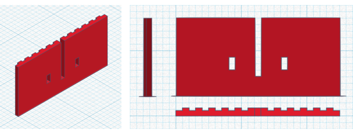
Figure 1: Object design. A 3D view (left) and 2D view (right) from the side, front, and top of the object design. The grid represents 1.0 mm x 1.0 mm, with 1.0 cm x 1.0 cm in bold. The wall is 25 mm x 12 mm x 1.2 mm (width x height x depth), and the ridges have a width of 1.0 mm, have a depth of 0.4 mm, and are separated by 1.0 mm. The windows have a width of 1.0 mm and a height of 2.0 mm. The 3D design can be found in Supplementary Coding File 1. Please click here to view a larger version of this figure.

Property/setting	Value
Filament	Polylactic acid (PLA), white
Nozzle diameter	0.4 mm
Layer thickness	0.2 mm
Nozzle temperature	210 °C
Cooling fan speed	100%
Printing speed	10 mm/s
Travel speed	10 mm/s
Bed Temperature	60 °C

Table 1: The 3D print settings. The settings and printer properties used for slicing the object design. For the second experiment, the fan speed was manually changed to 0%.

3. Performing the experiment

1. Start the 3D printer, and wait for the warm-up period to end.
2. The LSI measurement can be started at any moment, but to prevent unnecessary data saving, start the LSI measurement when the plastic starts to extrude.
3. Wait for the 3D printer to finish, and then stop the LSI measurement.
4. Load the resulting data into an image viewing software, and visually inspect the printed object. Compare the measured plastic polymer motions during printing with the final structural integrity and surface quality.

Results

A simple object was drawn as a test target for the experiments: a wall with ridges on the back, two windows, and a large hole (Figure 1). The object was sliced with the printer settings and properties listed in Table 1.

The LSI instrument was aligned with the 3D printer, and the experiment was performed. The user-friendly setup features an additional brightfield camera, which helps during alignment and allows for an easy comparison between the plastic extrusion and the measured polymer motion. The speckle and the brightfield cameras are both equipped with optical filters that prevent interference from the other channel. More technical details about the setup can be found in Supplementary File 1, and an explanation of the analysis routine is presented in Supplementary File 2. Highlights of the results of this experiment are shown in Figure 2, and the full movie can be found in Supplementary Movie 1. As shown before, the experiment can be performed just as well with a home-built instrument¹⁷.

Figure 2: Time-lapse of printing with a 100% cooling fan speed. Left: Brightfield, front-view image of the object when the printer is almost finished. The quality of the print looks good upon inspection; although the surface shows the layer lines, the overall designed geometry has been produced. Right: Four LSI snapshots from the white delineated region during the printing process; the blue arrows indicate the print head position at the time of the snapshot, as the LSI images do not correspond in time with the brightfield image. The lighter colors in each snapshot indicate increased polymer motion, which is observed in the most recently printed layers. Note that the region with enhanced motion (the welding zone) is multiple layers thick. The full detailed movie of the experiment is available in Supplementary Movie 1. Please click here to view a larger version of this figure.

Complementary to these results, the print was visually inspected; as expected for these commonly used polymer filaments and print settings, the quality was good. The designed geometry was, indeed, reproduced, and the surface was even, with a small line visible on each layer. With the LSI data, it was possible to gain in-depth insight into the printing process. The freshly extruded plastic was visible as highly mobile, and the mobility decreased gradually as it cooled down. The height of the area with high mobility (i.e., the welding zone) was four to five layers thick throughout the printing procedure, indicating a well-defined duration of layer fusion.

The experiment was repeated with the cooling fan speed manually adjusted to 0%. With this setting, the plastic did not cool down fast enough, which affected the print quality. Highlights of the results are shown in Figure 3, and the full detailed movie can be found in Supplementary Movie 2.

Figure 3: Time-lapse of printing with a 0% cooling fan speed. Left: Brightfield, front-view image of the object when the printer is almost finished. The visual quality of the print looks poor; the surface shows irregular layer lines and big blobs. Additionally, the overall designed geometry has been imperfectly reproduced; notably, the windows and holes are deformed. Right: Four LSI snapshots from the white delineated region during the printing process; the blue arrows indicate the print head position at the time of the snapshot, as the LSI images do not correspond in time with the brightfield image. The lighter colors in each snapshot indicate increased polymer motion, which can be observed throughout the whole object. The full detailed movie of the experiment is available in Supplementary Movie 2. Please click here to view a larger version of this figure.

In line with expectations, visual inspection of the 3D-printed construct indeed showed poor print quality. The layers were unevenly distributed, and the designed geometry was reproduced with deformations. A comparison of the brightfield images in Figure 2 and Figure 3 shows the major effect of the cooling fan on the surface quality and shape of the print result. The origin of this effect was determined by comparing the LSI results from Figure 2 and Figure 3. With a 100% cooling fan speed, enhanced polymer motion was observed in a region only a few layers below the extruded plastic. Therefore, each layer was liquified moderately a few times to achieve layer bonding without plastic flow. With the 0% cooling fan speed, enhanced polymer motion was observed through the whole object. Thus, each layer was liquified many times and extremely close to the freshly extruded plastic, resulting in a loss of geometric accuracy through plastic flow.

To gain a more quantitative view of the cooling fan effect in more moderate situations, the cooling fan speed was systematically varied. The object design was simplified to a wall of 25 mm x 12 mm x 0.8 mm (width x height x depth) without holes or ridges. The same print settings as in Table 1 were used. The experiment was performed 12 times, with cooling fan speeds of 0%, 20%, 40%, 60%, 80%, and 100%, each in duplicate. The resulting movies can be found in Supplementary Movies 3, Supplementary Movie 4, Supplementary Movie 5, Supplementary Movie 6, Supplementary Movie 7, and Supplementary Movie 8, as well as Supplementary Coding File 6, Supplementary Coding File 7, Supplementary Coding File 8, Supplementary Coding File 9, Supplementary Coding File 10, and Supplementary Coding File 11.

To quantitatively compare the welding zones for different fan speeds, advanced data analysis was performed on the LSI results. The goal of this data analysis was to obtain a height profile of the extent of the polymer motion in the welding zone. The associated fully commented MATLAB script can be found in Supplementary Coding File 4 and is described briefly. For every LSI image in the movie, a height profile is computed by taking the mean along the horizontal direction. The profiles of the images where the print head is in the ROI show a distinct peak around the welding zone. To exclusively select those profiles, only profiles with a peak above 8 dB are taken into account. Profiles in which this peak is too close to the edge of the ROI are also discarded. The peak positions of all profiles are subsequently aligned to give an average profile relative to the height at which the polymers are most mobile. The resulting profiles for the six different cooling fan speeds are plotted in Figure 4.

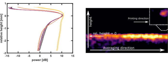
Figure 4: Height profiles for the systematic variation of the cooling fan speed. Left: The welding zone profiles for cooling fan speeds of 100% (black), 80% (blue), 60% (purple), 40% (red), 20% (orange), and 0% (yellow), obtained from the advanced data analysis script in Supplementary Coding File 4. The shaded region is the standard deviation between duplicate experiments. The right schematic explains the averaging procedure to obtain the profile of a typical LSI image. By aligning the maximums of the peaks of all the obtained profiles, the welding zone is obtained. The maximum of the welding zone (relative height = 0) is the height at which the polymers are most mobile. Full detailed LSI and brightfield movies of each experiment are available in Supplementary Movie 3, Supplementary Movie 4, Supplementary Movie 5, Supplementary Movie 6, Supplementary Movie 7,and Supplementary Movie 8. The objectprinted for this figure can be found in Supplementary Coding File 5, with corresponding G-code files in Supplementary Coding File 6. Please click here to view a larger version of this figure.

The welding zone profiles for 40%-100% cooling were nearly identical. The welding zone for 20% cooling had a shoulder reaching into several deeper layers. The welding zone for 0% cooling extended over the entire measured area. The height at which the polymers were most mobile lay in or slightly below the most recently printed layer. This phenomenon explains the presence of an LSI signal at positive relative heights, as there is printed material above the mobility peak. In all cases, the welding zone reached much deeper than the 0.2 mm layer thickness.

Supplementary File 1: LSI setup.xls. Hardware parameters of the LSI instrument used here. Please click here to download this File.

Supplementary File 2: LSI analysis.docx. Explanation of the conversion of the raw speckle images into LSI images. Please click here to download this File.

Supplementary Movie 1: LSI and brightfield movie of the experiment described in Figure 2. The movie is played at 12.5x real-time speed. The upper part is the LSI result, and the lower part is the synchronized brightfield view with the LSI ROI indicated. Please click here to download this Movie.

Supplementary Movie 2: LSI and brightfield movie of the experiment described in Figure 3. The movie is played at 12.5x real-time speed. The upper part is the LSI result, and the lower part is the synchronized brightfield view with the LSI ROI indicated. Please click here to download this Movie.

Supplementary Movie 3: The 100% cooling fan speed experiment described in Figure 4. The movie is played at 12.5x real-time speed. The upper part is the LSI result, and the lower part is the synchronized brightfield view with the LSI ROI indicated. Please click here to download this Movie.

Supplementary Movie 4: The 80% cooling fan speed experiment described in Figure 4. The movie is played at 12.5x real-time speed. The upper part is the LSI result, and the lower part is the synchronized brightfield view with the LSI ROI indicated. Please click here to download this Movie.

Supplementary Movie 5: The 60% cooling fan speed experiment described in Figure 4. The movie is played at 12.5x real-time speed. The upper part is the LSI result, and the lower part is the synchronized brightfield view with the LSI ROI indicated. Please click here to download this Movie.

Supplementary Movie 6: The 40% cooling fan speed experiment described in Figure 4. The movie is played at 12.5x real-time speed. The upper part is the LSI result, and the lower part is the synchronized brightfield view with the LSI ROI indicated. Please click here to download this Movie.

Supplementary Movie 7: The 20% cooling fan speed experiment described in Figure 4. The movie is played at 12.5x real-time speed. The upper part is the LSI result, and the lower part is the synchronized brightfield view with the LSI ROI indicated. Please click here to download this Movie.

Supplementary Movie 8: The 0% cooling fan speed experiment described in Figure 4. The movie is played at 12.5x real-time speed. The upper part is the LSI result, and the lower part is the synchronized brightfield view with the LSI ROI indicated. Please click here to download this Movie.

Supplementary Coding File 1: wall_with_holes.stl. The 3D design for the object described in Figure 1. Please click here to download this File.

Supplementary Coding File 2: wall_with_holes.gcode. The sliced object wall_with_holes.stl with the settings from Table 1. Please click here to download this File.

Supplementary Coding File 3: config.ini. The configuration file for the slicing software. Please click here to download this File.

Supplementary Coding File 4: AdvancedDataAnalysis_FanSpeed.m. The script to perform the advanced data analysis on the cooling fan sweep data and plot Figure 4. The script is fully commented. Please click here to download this File.

Supplementary Coding File 5: wall.stl. The 3D design of the object used to collect the data in Figure 4. Please click here to download this File.

Supplementary Coding File 6: wall_100%fan.gcode. The sliced object wall.stl with a 100% cooling fan speed. Please click here to download this File.

Supplementary Coding File 7: wall_80%fan.gcode. The sliced object wall.stl with an 80% cooling fan speed. Please click here to download this File.

Supplementary Coding File 8: wall_60%fan.gcode. The sliced object wall.stl with a 60% cooling fan speed. Please click here to download this File.

Supplementary Coding File 9: wall_40%fan.gcode. The sliced object wall.stl with a 40% cooling fan speed. Please click here to download this File.

Supplementary Coding File 10: wall_20%fan.gcode. The sliced object wall.stl with a 20% cooling fan speed. Please click here to download this File.

Supplementary Coding File 11: wall_0%fan.gcode. The sliced object wall.stl with a 0% cooling fan speed. Please click here to download this File.

Discussion

The experiments and results described in this research show that LSI is an easily applied tool that allows for a deeper understanding of layer bonding during additive manufacturing. LSI allows for the direct measurement of the polymer motion, which must be finely tuned to form a coherent material by the interpenetration and subsequent entangling of the polymer chains. The most common alternative for measuring layer bonding in situ is infrared imaging^3,4,5. This well-established method images the local surface temperature of the plastic^8,9, which is an indirect measurement of the polymer motion inside the material. With hotter plastic, the motion is faster, and the bonding becomes stronger. However, the relation between temperature and motion is not linear, as the printing temperatures cross the melting and glass transition temperatures^6,7. This non-trivial relationship can be directly observed in the LSI images; specifically, there is a sharp transition between the liquid-like top and the solid-like bottom regions, while the temperature gradient is expected to be far more gradual. Another drawback of IR imaging is that it measures the surface temperature only, while LSI measures polymer motion typically several millimeters deep inside the material.

Just like with IR imaging, this implementation of LSI is essentially a point-and-shoot method; it can be used in situ if the camera can be pointed at the region of interest. The versatile tripod and long working distance of 0.7 m give the freedom to use any available 3D printer. Crucially, LSI is sensitive to nanoscopic motions, and, thus, vibrations from the surroundings and the printing process itself have to be minimized¹⁷. For example, performing another task on the same table or slamming a door will cause interference. Therefore, one should carefully walk around the setup; however, room lights or airflow do not generally interfere with the process.

LSI gives detailed insight into the layer bonding process and can be applied as easily as IR imaging. We envision that LSI has great potential in aiding the development and understanding of advanced 3D printing methods. The cooling fan speed sweep shows a glimpse of what is possible by combining LSI with 3D printing. As discussed in the introduction, the optimal cooling speed is a balance between keeping the plastic molten for long enough to improve layer bonding but cooling it down fast enough to prevent flow. The 40%-100% cooling fan speed results were very similar; indeed, these fan speeds did not show any flow and produced a good surface quality. With the 0% cooling fan speed, the material started to flow away from the printed location, but ample layer bonding was observed in the LSI measurement. Based on our results, the 20% cooling fan speed could be optimal for achieving slightly improved layer bonding without compromising the surface quality. However, to draw conclusions that can be applied in practice, more cooling fan speeds between 0% and 40% must be assessed. It is also desirable to establish quantitative measures for the surface quality and material strength to gain an objective and complete view of the effects of polymer motion on the desired properties. With this addition, the approach could be made more powerful for evaluating creative 3D printing advances.

The exact settings that are chosen for the LSI analysis are not prone to critical errors as long as liquid-like plastic and solid-like plastic phases can be distinguished clearly. The polymer motion changes dramatically when crossing the melting and glass transition temperatures, so a broad range of LSI settings capture the contrast well. This can be easily tested with a test print of a straightforward object (e.g., a straight wall) with the 3D printer settings that are recommended by the material supplier. For more advanced LSI users, delving deeper into the frequency range can yield extra information, as different types of polymer motion can be quantitatively distinguished. For example, high-frequency polymer motion is associated with the highest temperatures, which are only present close to the printer head. Lower-frequency polymer motion is associated with moderate temperatures, which are present in a much larger area around the printer head and also for a much longer time¹⁷. Whether the degree of bonding for cumulative low-frequency polymer motion could be equal to that with short, high-frequency motion (e.g., with dynamic mechanical analysis) must be examined. Most other settings, like the colormap scaling, ROI, saving interval, and experiment length, are solely chosen to give a visually clear and appealing result. Regarding the 3D printing settings, there is also much freedom, as LSI allows the user to objectively assess the results of changing any of the settings. Notably, drastically changing the printing speed changes the interpretation of the LSI data. In this work, a slow printing and travel speed of 10 mm/s were used in order to capture multiple LSI images during one pass of the printer head. If a more common print speed of 60 mm/s for PLA were used, roughly one full layer would be printed per LSI image, and, thus, averaging within one layer would occur. If experimenting with high-end speeds such as 300 mm/s and faster, averaging over multiple layers would occur. Nevertheless, this is completely dependent on the exact print geometry and LSI settings and could be easily mitigated by an experienced LSI user through advanced machine design, adjusting the size of the field of view, or using a faster camera. Both approaches necessitate a more powerful laser, which, in combination with the reflective printer head, requires additional laser safety precautions. The relatively slow printing speed also has a positive influence on the layer bonding, as it was previously proven that heat transfer to the plastic increases with slower printing speeds⁵.

One possible new direction for this approach is the testing of novel materials; for example, LSI could be used to visualize the relevant transitions and objectively quantify the recommended printer settings that give a five-layer welding zone upon the application of the top layer. Another application could be to study the welding zone in specific situations where the print quality is not reliably good, such as for bridges, overhangs, or sharp corners. If the welding zone in difficult situations can be better understood, it should be possible to compensate in the G-code. It is already common practice to print the first layer hotter and slower than the rest of the layers to achieve good adhesion to the build plate¹⁸. We envision the use of similar dynamic G-code slicing where, for example, the fan cooling could be adjusted to produce corners or bridges. It should also be possible to print the outer wall material with a smoother finish and the rest of the material and infill rougher but stronger to maximize both the material strength and visual appearance.

This article has discussed the application of LSI to study the layer bonding process after plastic extrusion. The technique is excellent for this task, as it can visualize the underlying polymer motion without a priori assumptions in real-time during 3D printing. However, it does not give any information on the material cohesion, so additional testing will be required. The other drawbacks discussed are situational; the limited imaging speed of four LSI images per second can be increased with a bigger laser and additional laser safety measures, and the vibration sensitivity requires precautions or vibration reduction hardware. LSI can be performed with cheap and small digital cameras and lasers^19,20, which allows for integration into virtually every 3D printer for live quality control and dynamic tuning of the printing parameters. However, it makes more sense to employ LSI to develop thorough knowledge of layer bonding during 3D printing. If this understanding is used to develop more advanced slicing software, every consumer 3D printer could benefit from the knowledge gained.

Materials

List of materials used in this article

Name	Company	Catalog Number	Comments
3D-drawing sofware	Autodesk	TinkerCad	tinkercad.com
3D-Printer	Prusa3D	Original Prusa i3 MK3S
Advanced data analysis software	MathWorks	MATLAB R2018b
Image viewing sofware	National Institutes of Health	ImageJ 1.47v
LSI instrument	NanoMoI	NanoMoi allround	company to be founded 2023
Polylactic acid (PLA) filament	REAL	filament white 1,75 mm PLA 1 kg
Slicing software	Prusa3D	PrusaSlicer-2.5.0

References

- Daminabo, S. C., Goel, S., Grammatikos, S. A., Nezhad, H. Y., Thakur, V. K. Fused deposition modeling-based additive manufacturing (3D printing): Techniques for polymer material systems. Materials Today Chemistry. 16, 100248(2020).
- Lee, C. Y., Liu, C. Y. The influence of forced-air cooling on a 3D printed PLA part manufactured by fused filament fabrication. Additive Manufacturing. 25, 196-203 (2019).
- Seppala, J. E., Migler, K. D. Infrared thermography of welding zones produced by polymer extrusion additive manufacturing. Additive Manufacturing. 12, 71-76 (2016).
- Shmueli, Y., et al. Simultaneous in situ X-ray scattering and infrared imaging of polymer extrusion in additive manufacturing. ACS Applied Polymer Materials. 1 (6), 1559-1567 (2019).
- Dinwiddie, R. B., et al. Infrared imaging of the polymer 3D-printing process. Thermosense: Thermal Infrared Applications XXXVI. 9105, 910502(2014).
- Yousefpour, A., Hojjati, M., Immarigeon, J. P. Fusion bonding/welding of thermoplastic composites. Journal of Thermoplastic Composite Materials. 17 (4), 303-341 (2004).
- Peterson, A. M. Review of acrylonitrile butadiene styrene in fused filament fabrication: A plastics engineering-focused perspective. Additive Manufacturing. 27, 363-371 (2019).
- Menaka, M., Vasudevan, M., Venkatraman, B., Raj, B. Estimating bead width and depth of penetration during welding by infrared thermal imaging. Insight-Non-Destructive Testing and Condition Monitoring. 47 (9), 564-568 (2005).
- Möllmann, K. P., Vollmer, M. Infrared thermal imaging as a tool in university physics education. European Journal of Physics. 28 (3), 37(2007).
- Dela Torre, I. M., Montes, M. D. S. H., Flores-Moreno, J. M., Santoyo, F. M. Laser speckle based digital optical methods in structural mechanics: A review. Optics and Lasers in Engineering. 87, 32-58 (2016).
- Senarathna, J., Rege, A., Li, N., Thakor, N. V. Laser speckle contrast imaging: Theory, instrumentation and applications. IEEE Reviews in Biomedical Engineering. 6, 99-110 (2013).
- Buijs, J. J. Simpler, faster, and softer: Towards broad application of laser speckle imaging in art conservation and soft matter. Wageningen University and Research. , The Netherlands. PhD Thesis (2022).
- van der Kooij, H. M., et al. Morphing of liquid crystal surfaces by emergent collectivity. Nature Communications. 10 (1), 3501(2019).
- van Der Kooij, H. M., Broer, D. J., Liu, D., Sprakel, J. Electroplasticization of liquid crystal polymer networks. ACS Applied Materials & Interfaces. 12 (17), 19927-19937 (2020).
- van der Kooij, H. M., et al. Laser speckle strain imaging reveals the origin of delayed fracture in a soft solid. Science Advances. 4 (5), (2018).
- vander Kooij, H. M., Susa, A., García, S. J., vander Zwaag, S., Sprakel, J. Imaging the molecular motions of autonomous repair in a self-healing polymer. Advanced Materials. 29 (26), 1701017(2017).
- Buijs, J., Gucht, J. V. D., Sprakel, J. Fourier transforms for fast and quantitative laser speckle imaging. Scientific Reports. 9 (1), 13279(2019).
- Ehrmann, G., Ehrmann, A. Investigation of the shape-memory properties of 3D printed PLA structures with different infills. Polymers. 13 (1), 164(2021).
- Richards, L. M., Kazmi, S. S., Davis, J. L., Olin, K. E., Dunn, A. K. Low-cost laser speckle contrast imaging of blood flow using a webcam. Biomedical Optics Express. 4 (10), 2269-2283 (2013).
- Chen, H. L., Lai, C. L., Hsu, K. Y., Liu, W. M. Implementation of laser speckle imaging system with low cost consumer graded instrumentation for skin perfusion. 2016 IEEE International Conference on Consumer Electronics-Taiwan (ICCE-TW). , 1-2 (2016).
Reprints and Permissions