Multimodal Cross-Device and Marker-Free Co-Registration of Preclinical Imaging Modalities

Summary

The combination of multiple imaging modalities is often necessary to gain a comprehensive understanding of pathophysiology. This approach utilizes phantoms to generate a differential transformation between the coordinate systems of two modalities, which is then applied for co-registration. This method eliminates the need for fiducials in production scans.

Abstract

Integrated preclinical multimodal imaging systems, such as X-ray computed tomography (CT) combined with positron emission tomography (PET) or magnetic resonance imaging (MRI) combined with PET, are widely available and typically provide robustly co-registered volumes. However, separate devices are often needed to combine a standalone MRI with an existing PET-CT or to incorporate additional data from optical tomography or high-resolution X-ray microtomography. This necessitates image co-registration, which involves complex aspects such as multimodal mouse bed design, fiducial marker inclusion, image reconstruction, and software-based image fusion. Fiducial markers often pose problems for in vivo data due to dynamic range issues, limitations on the imaging field of view, difficulties in marker placement, or marker signal loss over time (e.g., from drying or decay). These challenges must be understood and addressed by each research group requiring image co-registration, resulting in repeated efforts, as the relevant details are rarely described in existing publications.

This protocol outlines a general workflow that overcomes these issues. Although a differential transformation is initially created using fiducial markers or visual structures, such markers are not required in production scans. The requirements for the volume data and the metadata generated by the reconstruction software are detailed. The discussion covers achieving and verifying requirements separately for each modality. A phantom-based approach is described to generate a differential transformation between the coordinate systems of two imaging modalities. This method showcases how to co-register production scans without fiducial markers. Each step is illustrated using available software, with recommendations for commercially available phantoms. The feasibility of this approach with different combinations of imaging modalities installed at various sites is showcased.

Introduction

Different preclinical imaging modalities have distinct advantages and disadvantages. For instance, X-ray computed tomography (CT) is well-suited for examining anatomical structures with different radio densities, such as bones and lungs. It is widely used due to its rapid acquisition speed, high three-dimensional resolution, relative ease of image assessment, and versatility with or without contrast agents^1,2,3. Magnetic resonance imaging (MRI) provides the most versatile soft tissue contrast without ionizing radiation⁴. On the other hand, tracer-based modalities like positron emission tomography (PET), single-photon emission computed tomography (SPECT), fluorescence-mediated tomography (FMT), and magnetic particle imaging (MPI) are established tools for quantitatively assessing molecular processes, metabolism, and the biodistribution of radiolabeled diagnostic or therapeutic compounds with high sensitivity. However, they lack resolution and anatomical information^5,6. Therefore, more anatomy-oriented modalities are typically paired with highly sensitive ones having their strength in tracer detection⁷. These combinations make the quantification of tracer concentrations within a specific region of interest possible^8,9. For combined imaging devices, modality co-registration is usually a built-in feature. However, it is also useful to co-register scans from different devices, e.g., if the devices were purchased separately or if a hybrid device is not available.

This article focuses on cross-modality fusion in small animal imaging, which is essential for basic research and drug development. A previous study¹⁰ points out that this can be achieved with feature recognition, contour mapping, or fiducials markers (fiducials). Fiducials are reference points for accurately aligning and correlating images from different imaging modalities. In special cases, fiducials can even be dots of Chinese ink on the skin of nude mice¹¹; however, often, an imaging cartridge with built-in fiducial markers is used. While this is a robust and well-developed method¹⁰, using it for every scan presents practical problems. MRI-detectable fiducials are often liquid-based and tend to dry out during storage. PET requires radioactive markers, the signal of which decays according to the emitter's half-life period, which is usually short for biomedical applications, necessitating preparation shortly before the scan. Other issues, such as the mismatch in the dynamic range of the signal from the fiducial marker and the examined object, strongly impact in vivo imaging. The wide range of dynamic contrast requires frequent adaptation of the marker signal strength to the object being examined. Consequently, while a weak marker signal may not be detected in the analysis, a strong marker signal may create artifacts that impair image quality. Additionally, to consistently include the markers, the field of view must be unnecessarily large for many applications, potentially leading to higher radiation exposure, larger data volumes, longer scan times, and, in some cases, lower resolution. This may affect the health of laboratory animals and the quality of the generated data.

Transformation and differential transformation
An image dataset consists of voxel data and metadata. Each voxel is associated with an intensity value (Figure 1A). The metadata includes a transformation specifying the dataset placement in the imaging device's coordinate system (Figure 1B) and the voxel size used to scale the coordinate system. Additional information, such as device type or scan date, can be optionally stored in the metadata. The mentioned transformation is mathematically called a rigid body transformation. Rigid body transformations are used to change the orientation or position of objects in an image or geometric space while preserving the distance between each pair of points, meaning the transformed object retains its size and shape while being rotated and translated in space. Any series of such transformations can be described as a single transformation consisting of a rotation followed by a translation. The formula used by the software to move from the data coordinate to the metric target coordinate is shown in Figure 1C, where R is an orthonormal rotation matrix, d and v are voxel indices and sizes, and t is a 3 x 1 translation vector¹². The rotation is detailed in Figure 1D.

Figure 1: 2D representation of an image dataset structure and placement in a global coordinate system. (A) An image dataset consists of voxel data and metadata. The transformation specifying the placement and voxel size are essential metadata components. (B) The image is rendered into the device's coordinate system. The necessary transformation to place the object consists of a rotation (blue) followed by a translation (green). (C) To move from the data coordinate to the target coordinate, the software uses this formula where R is an orthonormal rotation matrix, d, and v are voxel indices and sizes, and t is a 3 x 1 translation vector. (D) A rotation matrix (blue in plane A) represents the linear transformation of rotating points. Multiplying a point's coordinates by this matrix results in the new, rotated coordinates. Please click here to view a larger version of this figure.

A differential transformation is a rigid body transformation converting coordinates from one coordinate system to another, e.g., from PET to X-ray microtomography (µCT), and it can be computed using fiducial markers. At least three common points - the fiducials - are selected in both coordinate systems. From their coordinates, a mathematical transformation can be derived that converts the coordinates. The software uses the least squares method, which provides a best-fit solution to a system of equations with errors or noise in the measured data. This is called the Procrustes Problem¹³ and is solved using singular value decomposition. The method is reliable and robust because it leads to a unique and well-defined solution (if at least three non-collinear markers are given). Six free parameters are calculated: three for translation and three for rotation. In the following, we will use the term transformation matrix even though it technically consists of a rotation matrix and translation vector.

Each imaging device has its own coordinate system, and the software calculates a differential transformation to align them. Figure 2A,B describe how the differential transformation is determined, while Figure 2C,D describe how it is applied. The images of both modalities can have different dimensions and keep them in the process, as is shown in the example image with the fusion of CT and PET in Figure 2E.

Figure 2: Differential transformation. (A-D) Simplified to 2D. While applicable to other modalities, it is assumed that the modalities are CT and PET for this example. (A,C) A CT image with a red bounding box is positioned in the coordinate system. Applied to the same coordinate system, the PET image with a yellow bounding box is positioned deviating.(B) Using fiducial markers that can be located in both CT and PET, a differential transformation T can be determined. This is symbolized by the arrow. The differential transformation matrix is stored. (D) The previously saved differential transformation matrix T can then be applied to each PET image. This results in a new transformation that replaces the original transformation in the metadata. (E) A CT image fused with a PET image. The transformations in the metadata of both images refer to the same coordinate system. Please click here to view a larger version of this figure.

Method and requirements
For the presented method, a phantom containing markers visible in both modalities is scanned in both devices. It is then sufficient to mark these fiducials in the proposed software to calculate a differential transformation between the two modalities. The differential transformation must be created individually for each pair of devices. It can be saved and later applied to any new image, thereby eliminating the need for fiducial markers in subsequent scans. The final placement of the image in the coordinate system of another device can again be described as a transformation and be stored in the metadata of the image, replacing the original transformation there.

Four requirements for this method can be formulated: (1) Multimodal phantom: A phantom containing markers visible in both modalities must be available. A large selection of phantoms is commercially obtainable, and the use of 3D printing for phantom construction has been widely described¹⁴, even including the incorporation of radioisitopes¹⁵. The phantoms utilized in the following examples are listed in the Table of Materials. At least three non-collinear points are required¹⁶. The markers might be cavities that can be filled with an appropriate tracer, small objects made of a material that is easily detectable in each modality, or simply holes, cuts, or edges in the phantom itself as long as they can be identified in both modalities. (2) Multimodal carrier: A carrier, such as a mouse bed, is needed that can be fixed in a reproducible position in both devices. Ideally, it should not be possible to use it in a reversed position to avoid errors. The carrier is particularly important for in vivo imaging because it is needed to transport a sedated animal from one imaging device to the other without changing its position. Based on our experience, sedated mice are more likely to change their position in a flat mouse bed compared to a concave-shaped one. Additionally, a custom 3D-printed jig for holding the mouse's tibia to minimize motion has been previously suggested¹⁷. (3) Self-consistency: Each imaging device must provide the rotation and translation of the reconstructed volume in its reference frame in a reproducible and coherent manner. This also means that a coordinate system for the entire device is preserved when only a small region is scanned. It is part of the protocol to test an imaging device for its self-consistency. (4) Software support: The proposed software must be able to interpret the metadata (voxel size, translation, orientation) stored with the reconstructed volume provided by the device. The volume can be in DICOM, NIfTI, Analyze, or GFF file format. For an overview of various file formats, see Yamoah et al.¹².

While the co-registration of two modalities is described, the procedure is also applicable to three or more modalities, for example, by co-registering two modalities to one reference modality.

Protocol

The software steps of the protocol are to be performed in Imalytics Preclinical, which is referred to as the "analysis software" (see Table of Materials). It can load volumes as two different layers called "underlay" and "overlay"¹⁸. The underlay rendering is usually used to inspect an anatomically detailed data set on which a segmentation may be based; the overlay, which can be rendered transparently, can be used to visualize additional information within the image. Usually, the signal distribution of a tracer-based modality is displayed in the overlay. The protocol requires switching the selected layer several times. This is the layer that will be affected by the editing operations. The currently selected layer is visible in the dropdown list in the top toolbar between the mouse and window icons. One can press tab to switch between underlay and overlay, or select the desired layer directly from the dropdown list. The protocol will refer to scans (or images) used to test self-consistency and determine a differential transformation as "calibration scans", in contrast to "production scans" which are subsequently used for content-generating imaging. The modalities used in the protocol are CT and PET. However, as described earlier, this method applies to all preclinical imaging modalities capable of acquiring volumetric data.

1. Assembling the carrier and phantom

NOTE: A suitable multimodal carrier, e.g., a mouse bed, must be available on which the phantom can be fixed. See the discussion for suggestions, frequent problems, and troubleshooting regarding this assembly.

1. Prepare the fiducial markers in the phantom.
   NOTE: The specific preparation required varies depending on the modality and tracer used. For instance, many MRI phantoms contain cavities that need to be filled with water, whereas PET, as another example, requires a radioactive tracer.
2. Place the phantom in the carrier and secure it with a material, such as tape, that will not impair image quality.
   ​NOTE: The requirements for the phantom are detailed in the Introduction section.

2. Performing calibration scans and checking self-consistency

NOTE: This step needs to be repeated for each imaging device.

1. Acquire two scans with different fields of view.
   1. Place the carrier in the imaging device. Ensure it is placed in a reliable and reproducible manner.
   2. Scan according to the device manufacturer's instructions, using a large field of view that covers the entire phantom. This image will be referred to as "Image A" in the following steps.
      NOTE: It is important to include all fiducials, as this scan will also be used to calculate the differential transformation matrix.
   3. Remove the carrier from the imaging device and replace it.
      NOTE: This step ensures the carrier's placement in the device is reliable.
   4. If the imaging device does not support a limited field of view, i.e., always scans the entire field of view, one can reasonably assume self-consistency. Proceed directly to step 3.
   5. Perform a second scan according to the device manufacturer's instructions, this time using a significantly smaller field of view. This image will be called "Image B" in the following steps.
      NOTE: It is important to take two scans with different fields of view. The exact position of the field of view is not critical for image B, as long as some visible information, such as phantom structures or as many fiducials as possible, is included.
2. Load the underlay.
   1. Open the analysis software.
   2. Load image A as underlay: Menu File > Underlay > Load underlay. In the following dialog, choose the image file and click on open.
   3. If the 3D view is not present, press [Alt + 3] to activate it.
   4. Adjust the windowing: Press [Ctrl + W] and adjust the left and right vertical bars in the following dialog so that the phantom, or depending on the modality, the tracers, can be clearly distinguished. Click on Okay to close the dialog.
3. Load the overlay.
   1. Load image B as overlay: Menu File > Overlay > Load overlay. In the following dialog, choose the image file and click on open.
   2. Change the rendering method: Menu 3D-Rendering > Overlay mode > check Iso rendering.
      NOTE: Though tracer-based modalities like PET or SPECT are usually viewed with volume rendering, Iso rendering, in this case, allows for easier comparison of positions. The underlay was, by default, opened in Iso rendering.
   3. Activate the view of bounding boxes: Menu View > Show symbols > Show bounding box > Show underlay bounding box; Menu View > Show symbols > Show bounding box > Show overlay bounding box.
4. Check image alignment.
   1. Place the mouse pointer on the 3D view and use [Ctrl + mouse wheel] to zoom the view so that both bounding boxes are fully visible. Hold [Alt + left mouse button] while moving the mouse pointer to rotate the view.
   2. Switch the selected layer to overlay.
   3. Adjust the windowing and color table: Press [Ctrl + w]. In the dropdown list at the left of the following dialog, select Yellow. Adjust the range in the following dialog to a similar one that was chosen for the underlay, and then, change the setting in small steps until the yellow rendering is just visible within the white rendering. Click on Okay to close the dialog.
      NOTE: The rendering of Image A (underlay) is now depicted in white and surrounded by a red bounding box. The rendering of Image B (overlay) is depicted in yellow and surrounded by a yellow bounding box.
   4. Visually check if the imaging device and the method of placing the phantom are self-consistent as required. The phantom (or, depending on the modality, the tracers) should be fully aligned in underlay and overlay. The yellow rendering should be a subset of the white rendering.
      ​NOTE: The yellow bounding box should be smaller and within the red bounding box. See the Representative Results section for visual examples. If the alignment does not match, refer to the discussion for common placement problems and troubleshooting.

3. Calculation of the differential transformation

1. Load images of both modalities.
   1. Open the analysis software.
   2. Load the CT image A as underlay: Menu File > Underlay > Load underlay. In the following dialog, choose the image file and press open.
   3. Load the PET image A as overlay: Menu File > Overlay > Load Overlay. In the following dialog, choose the image file and press open.
   4. Show multiple slice views: Press [Alt + A], [Alt + S], and [Alt + C] to show axial, sagittal, and coronal slice views.
      NOTE: While technically, one plane would be sufficient to find the fiducials, the simultaneous view of all the planes allows for better orientation and quicker navigation.
2. Perform marker-based fusion.
   NOTE: Step 3.2 and step 3.3 are alternate methods to align underlay and overlay. Try step 3.2 first because it is easier to reproduce and potentially more accurate. Step 3.3 is a fallback if not enough markers are clearly discernible.
   1. Switch the view to only show the underlay: Menu View > Layer Settings > Layer Visibility > uncheck overlay; Menu View > Layer Settings > Layer Visibility > check underlay.
   2. Switch the selected layer to the underlay.
   3. If necessary, adjust the windowing: Press [Ctrl + W] and adjust the left and right vertical bars in the following dialog to better see the fiducials. Click on Okay to close the dialog.
   4. Activate the mouse action mode "create marker" by clicking the marker symbol on the vertical toolbar on the left side. The mouse pointer shows a marker symbol.
   5. Perform for each fiducial of the phantom: Navigate to a fiducial. To this end, place the mouse pointer over the view of a plane and use [Alt + mouse wheel] to slice through the planes. Place the mouse pointer on the center of the fiducial and left-click.
      1. This opens a dialog in which the software will suggest a name with consecutive numbers. Keep the suggested name, e.g., "Marker001," and click on ok to save the marker.
         NOTE: It is possible to use different names if you use the same marker names again for the overlay.
   6. Adjust the viewing settings to show the overlay: Menu View > Layer Settings > Layer Visibility > check overlay.
      NOTE: It is suggested to keep the view of the underlay activated, as it is helpful to stay orientated and be sure to identify the right marker in both modalities. If the two modalities are far out of sync or if the overlay is confusing, deactivate it: Menu View > Layer Settings > Layer Visibility > uncheck underlay.
   7. Switch the selected layer to overlay.
   8. Adjust the windowing: If the fiducial markers are not clearly visible, press [Ctrl + W] and adjust the left and right vertical bars in the following dialog so that the fiducials can be located as best as possible. Click on Okay to close the dialog.
   9. Perform for each fiducial of the phantom: Navigate to a fiducial. To this end, place the mouse pointer over the view of a plane and use [Alt + mouse wheel] to slice through the planes. Place the mouse pointer on the center of the fiducial and left-click.
      1. This opens a dialog in which the software will suggest a name with consecutive numbers. Keep the suggested name and click on ok to save the marker.
         NOTE: It is important to have the same name for matching software markers in underlay and overlay. This is ensured if you keep the suggested names and use the same order to create the markers in both modalities. If you change the names, make sure they match.
   10. Activate the views of both layers: Menu View > Layer Settings > Layer Visibility > check underlay; Menu View > Layer Settings > Layer Visibility > check overlay.
   11. Align the markers of underlay and overlay: Menu Fusion > Register overlay to underlay > Compute rotation and translation (markers). The following dialog shows the residual of fusion. Note this measurement and click on ok.
   12. Check the result of the alignment: The markers in the underlay and overlay should visually match. Check the discussion section for troubleshooting and notes on accuracy regarding the residual of fusion.
       NOTE: The transformation of the overlay has been changed. To display the details of the new overlay transformation, press [Ctrl + I].
3. If marker-based fusion is not possible, perform interactive fusion. If step 3.2 is completed, directly proceed to step 3.4.
   1. Activate the views of both layers: Menu View > Layer Settings > Layer Visibility > check underlay; Menu View > Layer Settings > Layer Visibility > check overlay.
   2. Activate the mouse mode "interactive image fusion" by clicking on the symbol on the vertical toolbar on the left side. The symbol consists of three offset ellipses with a point in the common center. The mouse pointer now shows this symbol.
   3. Ensure that the settings toolbar for the mouse mode appears in the upper area below the permanent toolbar. There are three checkboxes for underlay, overlay, and segmentation. Check overlay. Uncheck underlay and segmentation.
   4. Interactively align the overlay to the underlay: Perform rotations and translations on the different views until the underlay and overlay are aligned as best as possible:
      1. Rotation: Place the mouse pointer near the edge of a view (axial, coronal or sagittal); the mouse pointer symbol is now encircled by an arrow. Hold the left mouse button and move the mouse to rotate the overlay.
      2. Translation: Place the mouse pointer near the center of a view. The mouse pointer is not encircled. Hold the left mouse button and move the mouse to move the overlay.
4. Create and save the differential transformation: Menu Fusion > Overlay transformation > Create and save differential transformation. In the following dialog, select the original overlay file and click on Open. In the second dialog, enter a file name for the differential transformation and press Save.
   ​NOTE: The software needs the original overlay file to read the original transformation and then compute the differential transformation. We suggest saving the differential transformation matrix with a filename that specifies the imaging devices used.

4. Production imaging

1. Scan in both imaging devices.
   1. Fix the sample (e.g., a sedated laboratory animal) on the carrier.
      NOTE: It is important to ensure that the position of the sample within the carrier does not change between the two scans. 
   2. Place the carrier in the CT device. Ensure to place the carrier in the same way as was done during the calibration scan.
   3. Scan according to the instructions of the device's manufacturer.
   4. Place the carrier in the PET device. Ensure to place the carrier in the same way as was done during the calibration scan.
   5. Scan according to the instructions of the device's manufacturer.
2. Perform application of the differential transformation.
   1. Open the analysis software.
   2. Load CT file as underlay: Menu File > Underlay > Load underlay. In the following dialog, choose the CT image file and press ok.
   3. Load PET file as overlay: Menu File > Overlay > Load overlay. In the following dialog, choose the PET image file and press ok.
   4. Activate the views of both layers: Menu View > Layer Settings > Layer Visibility > check underlay; Menu View > Layer Settings > Layer Visibility > check overlay.
   5. Load and apply the previously saved differential transformation matrix: Menu > Fusion > Overlay transformation > Load and apply transform. Select the file containing the differential transformation matrix you saved in the calibration process and press open.
      NOTE: This step changes the metadata of the overlay.
   6. Save the altered overlay: Menu > File > Overlay > Save overlay. In the following dialog, enter a name and click on save.
      NOTE: It is recommended to keep the unaltered original data and, therefore, save the overlay under a new name.

Results

Figure 3 and Figure 4 provide examples of a phantom that is visible in CT and contains tubular cavities filled with a tracer, in this case, for SPECT. The phantom and the tracer used are listed in the Table of Materials.

Step 2 of the protocol outlines the calibration scans and verifies the self-consistency of each imaging device. The renderings from the two scans with different fields of view should be congruent for each device. Consequently, image B, depicted in yellow, should be a subset of image A, depicted in white. An example using CT is presented in Figure 3A. Tracer-based modalities like PET or SPECT are typically visualized with volume rendering (Figure 3B). However, Iso rendering facilitates easier position comparisons. Therefore, the protocol instructs users to switch the underlay and overlay to Iso rendering, regardless of the modality used. Thus, in the SPECT example, the yellow rendering should also be a subset of the white rendering (Figure 3C). In every instance, the yellow bounding box should be smaller and positioned within the red bounding box. If the alignment does not match, the discussion highlights common placement issues and provides troubleshooting suggestions.

Step 3 of the protocol describes how to determine the differential transformation between two modalities using fiducial markers. Since the tracer in tracer-based modalities is present as a volume, the user must determine appropriate points to use as a (point-shaped) fiducial marker. In Figure 4, a CT image of the phantom is loaded as underlay, and a SPECT image is loaded as underlay. The center of a curve of a tube inside the phantom is chosen as a fiducial marker for the CT underlay, as shown by Figure 4A-C in axial, coronal, and sagittal views. The corresponding point needs to be marked in the overlay, which is illustrated in Figure 4D-F in axial, coronal, and sagittal views. The software can now compute and apply the differential transformation to the overlay. This aligns the markers in both modalities, as is shown in Figure 4G,H.

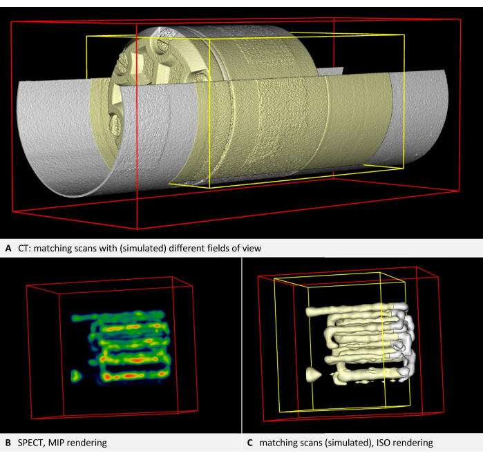
Figure 3: Images demonstrating self-consistency. (A) CT volume. Step 2.4 of the protocol requires checking the image alignment. According to the steps in the protocol, the underlay is rendered white, while the overlay and the bounding box of the overlay are rendered yellow. Both layers are in alignment (here, the second scan is simulated by a cropped copy of the first scan). (B) SPECT imaging of the phantom with tracer-filled tubes. Volume rendering with NIH color table. (C) SPECT image in ISO rendering. The underlay is rendered white, while the overlay and the bounding box of the overlay are rendered yellow. Both layers are in alignment (here, the second scan is simulated by a cropped copy of the first scan). Please click here to view a larger version of this figure.

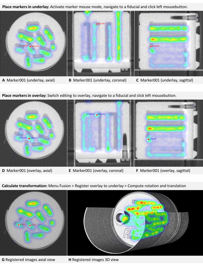
Figure 4: Placement of markers in CT and SPECT images. A CT image of the phantom is loaded as underlay. A SPECT image is loaded as an overlay and rendered using the NIH color table. (A-C) Step 3.2 of the protocol requires placing markers in the underlay. The center of a curve of a tube inside the phantom is chosen as fiducial, and Marker001 is placed there, as shown by a red dot in axial, coronal, and sagittal views. (D-F) The matching marker is placed in the overlay. (G) Axial view after the transformation. (H) 3D view of the fused modalities. Maximum intension projection rendering is used to make the SPECT tracer visible within the phantom. Please click here to view a larger version of this figure.

Discussion

A method for multimodal image co-registration that does not require fiducial markers for production scans is presented. The phantom-based approach generates a differential transformation between the coordinate systems of two imaging modalities.

Residual of fusion and validating the differential transformation
Upon calculating the differential transformation, the software displays a residual of fusion in millimeters, representing the root mean square error¹⁹ of the transformation. If this residual exceeds the order of magnitude of the voxel size, it is advisable to inspect the datasets for general issues. However, as all images have slight distortions, the residual cannot become arbitrarily small; it only reflects the fit of the markers used. For example, a co-registration with three markers may result in a smaller residual on the same datasets than a transformation with four well-distributed markers. This occurs because the markers themselves may be overfitted when fewer fiducials are employed. The accuracy across the entire dataset improves with a greater number of markers.

The quantitative accuracy of the method depends on the specific pair of devices used. The calculated differential transformation between the coordinate systems of two devices can be validated following these steps: Adhering to step 4 of the protocol, but using the phantom with fiducial markers as the "sample" again. Placing the phantom in any position, ensuring it's different from the one used for estimating the differential transformation. It's also possible to use a different phantom suitable for the respective modalities if one is available. Next, applying the differential transformation determined earlier (step 4.2.5) to align the two modalities. Then, placing markers on the images from both modalities as per step 3.2 of the protocol. To calculate the fusion residual for these markers, click on Menu Fusion > Register Overlay to Underlay > Showing Residual Score.

The residual error describes the average misplacement of the signal and should be in the order of the voxel size. Concrete acceptance thresholds are application-dependent and may depend on several factors, such as the stiffness and accuracy of the imaging systems but can also be affected by image reconstruction artifacts.

Troubleshooting self-consistency
Often, difficulties with self-consistency arise from unreliable placement. A common error is placing the carrier in a laterally reversed position. Ideally, it should be mechanically inserted into the imaging device in only one direction. If this is not feasible, comprehensible markings should be added for the user. Another frequent issue is the possibility of movement in the longitudinal axis, making axial positioning unreliable. Using a spacer that can be attached at one end to secure the mouse bed in place is recommended. Custom spacers can, for example, be quickly and easily created by 3D printing them. However, some devices cannot provide self-consistency with varying fields of view. In such cases, contacting the vendor is advised, who should confirm the incompatibility and potentially address it in a future update. Otherwise, the method remains reliable if an identical field of view is maintained for all scans, including calibration and production imaging.

For some production scans with deviating placement, transformation to the calibrated position is possible, if sufficient carrier structure is discernible. For in vivo imaging, the sedated animal must remain in one carrier, and constructing a single carrier that fits securely in both devices is not always achievable. Often, a mouse bed for a tracer-based modality is used, and then placement is improvised into a CT device. For instance, in Figure 5A, an MPI mouse bed was placed atop a CT mouse bed due to mechanical constraints. Axial leeway and the possibility of rolling make this positioning unreliable. In such cases, it is recommended to design an adapter that replaces the lower mouse bed and allows for an interlocking fit. It may, for example, use trunnions attached to the lower part and additional holes in the bottom of the upper mouse bed.

However, retrospective correction for existing images is possible, as the mouse bed is detectable in the CT image. The protocol necessitates calibration scans, followed by calculating a differential transformation of the overlay to the underlay. The procedure is similar but must also map each individual production CT scan to the calibration scan, using the mouse bed structures as fiducials.

Figure 5: Troubleshooting placement. (A) An MPI mouse bed is placed on top of a CT mouse bed. Hence, the position in the CT cannot be reliably reproduced. Self-consistency can be achieved by fusing each CT image to the reference CT image used for estimating the differential transformation. (B-D) Simplified to 2D. (B) Each production CT image is loaded as an overlay and registered to the reference CT image (underlay) using structures of the mouse bed visible in the CT. The corrected production CT image is now consistent with the reference CT and can be used with the differential transformation T. (C) An MPI overlay is registered to the reference CT image using the fiducial markers of a phantom. (D) The multimodal images are assembled. For this purpose, each CT image is mapped to the reference position with its individual differential transformation. Subsequently, the MPI overlay is also registered to the reference position using the differential transformation, which is valid for all images of the device. Please click here to view a larger version of this figure.

To map the production CT scans to the calibration scan, refer to section 3 of the protocol, incorporating the following modifications. For clarity, the description continues using the example of a CT underlay and MPI overlay: In step 3.1, load the CT calibration scan (image A) as the underlay and the CT scan to be corrected as the overlay. Utilize structures of the MPI mouse bed either as markers for step 3.2 or as visual references for step 3.3. Bypass step 3.4, but save the overlay represents the corrected CT volume (Menu File > Overlay > Saving overlay as). In the subsequent dialog box, input a new name and click on save. Close the overlay by navigating to Menu File > Overlay > Closing overlay. Load the next CT scan that requires correction as the overlay and resume the procedure from step 3.2 of the protocol. The concept underlying this step is illustrated in Figure 5B.

The mouse bed is now virtually aligned identically to the calibration scan in all the recently saved CT volumes. As part of the standard procedure, the calibration scan is registered to the MPI images using the differential transformation T (Figure 5C). To subsequently merge the CT image with MPI, always use the corrected CT volume (Figure 5D).

Troubleshooting flipped images and scaling
The registration method introduced here assumes reasonably accurate image quality and only adjusts rotation and translation. It does not correct for flipped images or incorrect scaling. However, these two issues can be addressed manually prior to calculating the differential transformation.

Inconsistencies between data formats from different manufacturers may cause some datasets, particularly those in DICOM format, to be displayed as mirror-inverted in the software. As phantoms and mouse beds are often symmetrical, this issue may not be immediately apparent. Detecting flipped images is easier when the scan contains recognizable lettering in the respective modality, such as the raised lettering in the correct orientation seen in the phantom in Figure 3H. In the example illustrated in Figure 6, CT data is loaded as the underlay, and MPI data is loaded as the overlay. It is an in vivo scan of a mouse placed in an MPI mouse bed with attached fiducial markers. The MPI mouse bed is situated on top of a µCT mouse bed (Figure 6A). By adhering to the protocol and marking the fiducials in both the underlay and overlay in a consistent direction of rotation, a visibly incongruous result is produced (Figure 6B). Upon closer inspection, however, the problem can be identified. The fiducials form an asymmetrical triangle. Observing the sides of the triangle in the axial view (Figure 6C, D) from the shortest to the middle to the longest, a clockwise rotation is evident in the CT data, while a counterclockwise rotation is apparent in the MPI data. This demonstrates that one of the images is laterally inverted. In this instance, we assume the CT data to be accurate. To rectify the MPI overlay, the image is flipped: to do that, switch the selected layer to overlay and click on Menu Edit > Flip > Flip X. The differential transformation calculated by the software encompasses all necessary rotations, so "Flip X" is sufficient even if the image appears flipped in another direction.

Figure 6: Troubleshooting transformation. CT data are loaded as underlay with a voxel size of 0.240 mm, and MPI data as overlay with a voxel size of 0.249 mm. The mouse bed contains fiducial markers. (A) 3D view of the uncorrected overlay image. The fiducials in the CT underlay are indicated by arrows. The fiducials in the MPI overlay are visible as spheres in the NIH color table. (B) Mismatched result of a transformation performed without appropriate corrections. Residual of fusion = 6.94 mm. (C) Measurement of the distances between the fiducials in CT. Clockwise rotation from the shortest to the longest distance. (D) Measurement of the distances between the fiducials in MPI. Counter-clockwise rotation from the shortest to the longest distance. Comparison with the CT measurements results in a scaling factor of 0.928774. (E) Corrected overlay after flipping and scaling. (F) Transformation with matching results in 3D view. (G) Transformation with matching results in axial view. Residual of fusion = 0.528 mm. Please click here to view a larger version of this figure.

Datasets with incorrect voxel sizes can also be corrected manually. Since the dimensions of the phantom should be known, this can be verified in the image. The simplest method is using an edge of known length. Press [Ctrl + right mouse button] at one end of an edge, and while holding the button down, move the mouse pointer to the other end of the edge and release the button. In the subsequent dialog, the software displays the length of the measured distance in the image. In the example illustrated in Figure 6, it is apparent that the sizes are not congruent when comparing the distances between the fiducials in both modalities (Figure 6C,D). Again, the CT data is assumed to be accurate. To modify the scaling, a scaling factor (SF) is computed. As the ratio of the lengths (CT/MPI) is not precisely identical for each side of the triangle, the mean quotient is calculated: SF = ((l_1CT/l_1MPI) + (l_2CT/l_2MPI) + (l_2CT/l_2MPI)) / 3.

Subsequently, adjust the voxel size of the overlay by multiplying each dimension by SF. To achieve this, switch the selected layer to overlay and open Menu Edit > Change Voxel Sizes. Compute each dimension, enter the value, and then click on OK. The result of both corrections is shown in Figure 6E. Following this, the overlay is registered to the underlay according to the protocol. The resulting alignment is displayed in Figure 6F,G. While this provides a quick solution for correcting an existing scan, we recommend calibrating the imaging device for production use.

Limitations
This method is limited to spatial co-registration of existing volumetric data composed of cube-shaped voxels. It does not include a reconstruction process that computes the volume from raw data generated by the imaging device (e.g., projections in CT). Various image enhancement techniques are associated with this step, such as iterative methods^20,21 and the application of artificial intelligence²¹. Although the described method is, in principle, applicable to all modalities that produce 3D images with cube-shaped voxels, it cannot be employed for fusing 3D data with 2D data, like an MRI volume combined with 2D infrared thermography²² or fluorescence imaging, which may be relevant in image-guided surgery applications. The registration of 3D data does not correct for distortions, such as those that occur in MRI images at the coil edge. While not mandatory, optimal results are achieved when distortions are corrected during the reconstruction process. The automated transformation also does not address flipped images or incorrect scaling. However, these two issues can be manually resolved as outlined in the troubleshooting section.

Significance of the method
The proposed method eliminates the need for fiducial markers in production scans, offering several advantages. It benefits modalities for which marker maintenance or frequent replacement is required. For example, most MRI markers are based on moisture but tend to dry out over time, and radioactive PET markers decay. By removing the necessity for fiducials in production scans, the field of view can be reduced, leading to shorter acquisition times. This is helpful in high-throughput settings to reduce costs and to minimize x-ray dose in CT scanning. A decreased dose is desirable because radiation can impact the biological pathways of test animals in longitudinal imaging studies²³.

Moreover, the method is not limited to specific modalities. The trade-off for this versatility is that fewer steps are automated. A previously published method for fusing µCT and FMT data employs built-in markers in a mouse bed for every scan and can perform automated marker detection and distortion correction during reconstruction²⁴. Other methods eliminate the need for markers by utilizing image similarity. While this approach yields good results and can also correct distortions²⁵, it is only applicable if the two modalities provide similar enough images. This is usually not the case in the combination of an anatomically detailed modality and a tracer-based modality. However, these combinations are necessary for assessing the pharmacokinetics of targeted agents²⁶, which have applications in areas such as anticancer nanotherapy^{27, 28}.

Because quality control is less rigorous in preclinical compared to clinical applications, misalignment of combined imaging devices is a recognized issue²⁹. Data affected by this misalignment could be improved retrospectively by scanning a phantom and determining the differential transformation, potentially reducing costs and minimizing animal harm. In addition to the demonstrated method that employs fiducial markers to calculate a differential transformation, which is then applied to production scans, further possibilities for image fusion are described and used. An overview, which includes references to various available software, can be found in Birkfellner et al.³⁰.

In conclusion, the presented method offers an effective solution for multimodal image co-registration. The protocol is readily adaptable for various imaging modalities, and the provided troubleshooting techniques enhance the method's robustness against typical issues.

Materials

List of materials used in this article

Name	Company	Catalog Number	Comments
177Lu			radiotracer
Custom-build MPI mousebed
Hot Rod Derenzo	Phantech LLC. Madison, WI, USA	D271626	linearly-filled channel derenzo phantom
Imalytics Preclinical 3.0	Gremse-IT GmbH, Aachen, Germany		Analysis software
Magnetic Insight	Magnetic Insight Inc., Alameda, CA, USA		MPI Imaging device
Quantum GX microCT	PerkinElmer		µCT Imaging device
U-SPECT/CT-UHR	MILabs B.V., CD  Houten, The Netherlands		CT/SPECT Imaging device
VivoTrax (5.5 Fe mg/mL)	Magnetic Insight Inc., Alameda, CA, USA	MIVT01-LOT00004	MPI Markers