We report detailed procedures for an invasive plant biomass estimation method that utilizes data obtained from unmanned aerial vehicle (UAV) remote sensing to assess biomass and capture the spatial distribution of invasive species. This approach proves highly beneficial for conducting hazard assessment and early warning of invasive plants.
A subscription to JoVE is required to view this content. Sign in or start your free trial.
Method Article
Computer Vision-Based Biomass Estimation for Invasive Plants
In This Article
Summary
Abstract
We report on the detailed steps of a method to estimate the biomass of invasive plants based on UAV remote sensing and computer vision. To collect samples from the study area, we prepared a sample square assembly to randomize the sampling points. An unmanned aerial camera system was constructed using a drone and camera to acquire continuous RGB images of the study area through automated navigation. After completing the shooting, the aboveground biomass in the sample frame was collected, and all correspondences were labeled and packaged. The sample data was processed, and the aerial images were segmented into small images of 280 x 280 pixels to create an image dataset. A deep convolutional neural network was used to map the distribution of Mikania micrantha in the study area, and its vegetation index was obtained. The organisms collected were dried, and the dry weight was recorded as the ground truth biomass. The invasive plant biomass regression model was constructed using the K-nearest neighbor regression (KNNR) by extracting the vegetation index from the sample images as an independent variable and integrating it with the ground truth biomass as a dependent variable. The results showed that it was possible to predict the biomass of invasive plants accurately. An accurate spatial distribution map of invasive plant biomass was generated by image traversal, allowing precise identification of high-risk areas affected by invasive plants. In summary, this study demonstrates the potential of combining unmanned aerial vehicle remote sensing with machine learning techniques to estimate invasive plant biomass. It contributes significantly to the research of new technologies and methods for real-time monitoring of invasive plants and provides technical support for intelligent monitoring and hazard assessment at the regional scale.
Introduction
In this protocol, the proposed method of invasive biomass estimation based on UAV remote sensing and computer vision can reflect the distribution of invasive organisms and predict the degree of invasive biohazard. Estimates of the distribution and biomass of invasive organisms are critical to the prevention and control of these organisms. Once invasive plants invade, they can damage the ecosystem and cause huge economic losses. Quickly and accurately identifying invasive plants and estimating key invasive plant biomass are major challenges in invasive plant monitoring and control. In this protocol, we take Mikania micrantha as an example to explore an invasive plant biomass estimation method based on unmanned aerial remote sensing and computer vision, which provides a new approach and method for the ecological research of invasive plants and promotes the ecological research and management of invasive plants.
At present, the biomass measurement of Mikania micrantha is mainly done by manual sampling1. The traditional methods of biomass measurement need a lot of workforce and material resources, which are inefficient and limited by the terrain; it is difficult to meet the needs of regional biomass estimation of Mikania micrantha. The major advantage of using this protocol is that it provides a method for quantifying regional invasive plant biomass and spatial distribution of invasive plants in a way that does not take into account the sampling limitations of the area and eliminates the need for manual surveys.
UAV remote sensing technology has achieved certain results in plant biomass estimation and has been widely used in agriculture2,3,4,5,6,7, forestry8,9,10,11, and grassland12,13,14. UAV remote sensing technology has the advantages of low cost, high efficiency, high precision, and flexible operation15,16, which can efficiently obtain remote sensing image data in the study area; then, the texture feature and vegetation index of remote sensing image are extracted to provide data support for the estimation of plant biomass in large area. Current plant biomass estimation methods are mainly categorized into parametric and nonparametric models17. With the development of machine learning algorithms, nonparametric machine learning models with higher accuracy have been widely used in remote sensing estimation of plant biomass. Chen et al.18 utilized mixed logistic regression (MLR), KNNR, and random forest regression (RFR) to estimate the aboveground biomass of forests in Yunnan Province. They concluded that the machine learning models, specifically KNNR and RFR, resulted in superior outcomes compared to MLR. Yan et al.19 employed RFR and extreme gradient boosting (XGBR) regression models to assess the accuracy of estimating subtropical forest biomass using various sets of variables. Tian et al.20 utilized eleven machine-learning models to estimate the aboveground biomass of varying mangrove forest species in Beibuwan Bay. The researchers discovered that the XGBR method was more effective in determining the aboveground biomass of mangrove forests. Plant biomass estimation using man-machine remote sensing is a well-established practice, however, the use of UAV for biomass estimation of the invasive plant Mikania micrantha has yet to be reported both domestically and internationally. This approach is fundamentally different from all previous methods of biomass estimation for invasive plants, especially Mikania micrantha.
To sum up, UAV remote sensing has the advantages of high resolution, high efficiency, and low cost. In the feature variable extraction of remote sensing images, texture features combined with vegetation indexes can obtain better regression prediction performance. Nonparametric models can obtain more accurate regression models than parametric ones in plant biomass estimation. Therefore, to calculate the null distribution of invasive plants and their biomass precisely, we suggest the following outlined procedures for the invasive plant biomass experiment that relies on remote sensing using UAVs and computer vision.
Access restricted. Please log in or start a trial to view this content.
Protocol
1. Preparation of datasets
- Selecting the research object
- Select test samples based on the focus of the experimental study, considering options like Mikania micrantha or other invasive plants.
- Collecting UAV images
- Prepare square plastic frames of size 0.5 m*0.5 m and quantity 25-50, depending on the size of the area studied.
- Employ a random sampling approach to determine soil sampling locations in the study area using a sufficient number of biomass samples. Position the sample frame horizontally over the vegetation, fully encompassing the plants with a minimum separation distance of 2 m between each plant.
- Use a drone and a camera to form a UAV remote-sensing filming system, as shown in Figure 1.
- Use the UAV to plot the route within the specified study area. The route planning setup is shown in Figure 2.
- Establish a heading and side overlap rate of 70%, capture photos at uniform time intervals of 2 s, maintain the camera angle perpendicular to the ground at 90°, and position the camera altitude at 30 m. This resulted in continuous visible image data of the study area with a single image resolution measuring 8256 x 5504 pixels, as depicted in Figure 3.
- Store aerial imagery for subsequent processing with Python software for biomass estimation.
- Collecting the aboveground biomass
- Collect the aboveground biomass of Mikania micrantha manually within each sample plot after completing the drone data collection. Bag them and label each bag accordingly.
- When collecting Mikania micrantha, prevent sample plots from moving. First, cut the Mikania micrantha along the inside edge of the sample plot.
- Then, cut the rhizome of the Mikania micrantha from the bottom. Remove any dirt, rocks, or other plants that are mixed in. Finally, bag and label the samples.
- Bring the collected samples of invasive plants from step 1.3.1 to the laboratory. Air-dry all the collected samples to evaporate most of the moisture.
- To further remove moisture from air-dried samples, use an oven. Set the temperature to 55 °C. Dry the samples for 72 h, then weigh each sample on an electronic balance and record the biomass data in grams (g).
- Place the electronic balance in an undisturbed environment, weigh, calibrate, and continue weighing. Place bags of Mikania micrantha on the electronic balance, wait for the readings to stabilize, and record the readings.
- Weigh the Mikania micrantha every hour until the mass no longer changes and record the reading minus the weight of the bag as the measured mass of that sample. Calculate the aboveground biomass of the invasive plant using the formula below:

where B represents the biomass of Mikania micrantha in grams per square meter (g/m2), M is the weight of the measured Mikania micrantha, measured in grams (g), S corresponds to the area of the sample plot in square meters (m2).
- Collect the aboveground biomass of Mikania micrantha manually within each sample plot after completing the drone data collection. Bag them and label each bag accordingly.
- Creating a dataset
- Extract the RGB image corresponding to the sample image from the original UAV image. Divide it into a grid of 280 × 280 pixels using Python programming (Supplementray Figure 1).
- Segment the raw image data into smaller images of the same size as the sample images using Python programming. Use the sliding window method for segmentation, setting the horizontal and vertical steps to 280 pixels.
- From the small images segmented in step 1.4.2, randomly select 880 invasive plant images and 1500 background images to create a dataset. Then, split this dataset into training, validation, and test sets in a 6:2:2 ratio (Supplementray Figure 2).
2. Identification of Mikania micrantha
- Preparing the software
- Go to Anaconda's official website (https://www.anaconda.com/) and download and install Anaconda. Then, head to PyCharm's website (https://www.jetbrains.com/pycharm/) and download the PyCharm IDE.
- Creating a Conda environment.
- Open the Anaconda Prompt command line after installing Anaconda, then type conda create -n pytorch python==3.8 to create a new Conda environment. After the environment is created, enter conda info --envs to confirm that the pytorch environment exists.
- Open the Anaconda Prompt and activate the pytorch environment by entering conda activate pytorch. Check the current (Compute Unified Device Architecture)CUDA version by typing nvidia-smi. Then, install PyTorch version 1.8.1 by running the command conda install pytorch==1.8.1 torchvision==0.9.1 torchaudio==0.8.1 cudatoolkit=11.0 -c pytorch.
- Runs for model recognition
NOTE: Use PyTorch to build the Mikania micrantha recognition model used in this paper. The network model employed is ResNet10121, which remains consistent with the original paper in its architecture. Modifications are made to the network's output section to meet the requirements for chamomile recognition.- Preprocess the images to prepare them for model input. Resize the images from 280 x 280 pixels to 224 x 224 pixels and normalize them to ensure they meet the model's size requirements using the following code:
transform = transforms.Compose([
transforms.Resize((224, 224)),
transforms.ToTensor(),
transforms.Normalize([0.485, 0.456, 0.406], [0.229, 0.224, 0.225])]) - Perform image feature extraction and reduce dimensionality using a convolutional neural network.
- First, initialize the convolutional layer for the initial feature extraction through self.conv1. With this convolutional layer, the original image is convolved into a feature map with self.in_channel channels for extracting initial features (Supplementary Figure 3A).
NOTE: Advanced features are extracted in a convolution operation on the residual passes. These layers are produced by invoking the _make_layer function, which comprises a sequence of residual blocks. Each residual block consists of convolution, batch normalization, and activation functions to gradually extract sophisticated features (Supplementary Figure 3B). - Use the layer's function to modify the channel number for dimensionality reduction via 1x1 convolution. This operation decreases the computational load while preserving significant features (Supplementary Figure 3C).
NOTE: Overall, ResNet101 performs feature extraction by using various convolutional layers, and dimensionality reduction is achieved through 1x1 convolutional layers within the residual block. This approach allows the network to learn features more deeply and avoid the issue of gradient vanishing, thus enabling more efficient learning and representation of image features for complex tasks. - After convolutions and pooling operations, input the high-quality features into a fully connected layer.
NOTE: In the ResNet architecture, feature extraction takes place in the convolutional layer. These features are subsequently sent to the fully-connected (FC) layer for classification (Supplementary Figure 4). The operation self.avgpool(x) performs adaptive average pooling to reshape the tensor to a fixed size. The operation torch.flatten(x, 1) spreads the tensor into a one-dimensional vector, and self.fc(x) applies the fully connected layer to the flattened vector, ultimately serving as the final step for classification. This process effectively passes the extracted features through the convolutional layer, transforming them into a format suitable for classification via the fully connected layer. - Use the Softmax function to obtain the final output based on the three classification requirements.
- First, initialize the convolutional layer for the initial feature extraction through self.conv1. With this convolutional layer, the original image is convolved into a feature map with self.in_channel channels for extracting initial features (Supplementary Figure 3A).
- Train a multi-class recognition model with the dataset from step 1.4. Set the number of iterations to 200 and an initial learning rate of 0.0001. Reduce the learning rate by a third every 10 iterations with a batch size of 64. Save the optimal model parameters automatically after each iteration (Supplementary Figure 5).
- Employ a meticulously trained recognition model and systematically traverse the original image from step 1.2.2 for identification purposes.
- Configure horizontal and vertical steps precisely at 280 pixels, resulting in the generation of a comprehensive distribution map highlighting the presence of invasive flora within the boundaries of the study area. Present the selected results visually as shown in Figure 4.
NOTE: The initial image is preprocessed by segmenting it into smaller chunks, classifying each chunk using a trained deep learning model, and combining the results into an output image. If a chunk is classified as an invasive plant, the corresponding location on the output image is set to 255. The resulting output image is saved as a grayscale image file. The specific implementation code is shown in Supplementary Figure 6.
- Configure horizontal and vertical steps precisely at 280 pixels, resulting in the generation of a comprehensive distribution map highlighting the presence of invasive flora within the boundaries of the study area. Present the selected results visually as shown in Figure 4.
- Preprocess the images to prepare them for model input. Resize the images from 280 x 280 pixels to 224 x 224 pixels and normalize them to ensure they meet the model's size requirements using the following code:
3. Estimation of invasive plant biomass
- Perform simple data augmentation with the RandomResizedCrop and RandomHorizontalFlip functions (Supplementary Figure 7) to extend the image set created in step 1.2 and extract the six vegetation indices commonly used for estimating biomass, which are RBRI, GBRI, GRRI, RGRI, NGBDI, and NGRDI. Refer to Table 1 for the calculation formulas for these indices.
- Create a K-nearest neighbor regression (KNNR)22 model using the output of the model to ensure precise estimation of the biomass of invasive plants. Use the extracted vegetation indices as inputs for the estimation model.
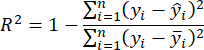
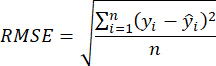
- Use the coefficient of determination R2 and Root Mean Square Error (RMSE)23 to assess the model's accuracy, which is calculated as follows:
NOTE: The K-Nearest Neighbor Regression (KNNR) algorithm is a nonparametric machine learning technique used to solve regression problems. Its fundamental concept is to predict outcomes by determining the closest K neighbors in feature space based on input sample distances. Key benefits of using KNNR include its simplicity and ease of understanding, and it requires no training phase. Additionally, KNNR does not make excessive assumptions about the data's distribution. KNNR can be applied in regression issues to anticipate continuous objective variables and precisely evaluate the biomass of invasive plants. - Employ the aboveground biomass estimation model chosen in step 3.2 and scan through the invasive plant distribution map from step 2.3.4 with horizontal and vertical strides of 280 pixels.
Access restricted. Please log in or start a trial to view this content.
Results
We show representative results of a computer vision-based method for the estimation of invasive plants, which is implemented in a programmatic way on a computer. In this experiment, we evaluated the spatial distribution and estimated the biomass of invasive plants in their natural habitats, using Mikania micrantha as a research subject. We utilized a drone camera system to acquire images of the research site, a portion of which is exhibited in Figure 3. We utilized the ResNet101 con...
Access restricted. Please log in or start a trial to view this content.
Discussion
We present the detailed steps of an experiment on estimating the biomass of invasive plants using UAV remote sensing and computer vision. The main process and steps of this agreement are shown in Figure 7. Proper sample quality is one of the most crucial and challenging aspects of the program. This importance holds true for all invasive plants as well as any other plant biomass estimation experiments24.
To identify the distribution of ...
Access restricted. Please log in or start a trial to view this content.
Disclosures
The authors have nothing to disclose.
Acknowledgements
The author thanks the Chinese Academy of Agricultural Sciences and Guangxi University for supporting this work. The work was supported by the National Key R&D Program of China (2022YFC2601500 & 2022YFC2601504), the National Natural Science Foundation of China (32272633), Shenzhen Science and Technology Program (KCXFZ20230731093259009)
Access restricted. Please log in or start a trial to view this content.
Materials
| Name | Company | Catalog Number | Comments |
|---|---|---|---|
| DSLR camera | Nikon | D850 | Sensor type: CMOS; Maximum number of pixels: 46.89 million; Effective number of pixels: 45.75 million; Maximum resolution 8256 x 5504. |
| GPU - Graphics Processing Unit | NVIDIA | RTX3090 | |
| Hexacopter | DJI | M600PRO | Horizontal flight: 65 km/h (no wind environment); Maximum flight load: 6000 g |
| PyCharm | Python IDE | 2023.1 | |
| Python | Python | 3.8.0 | |
| Pytorch | Pytorch | 1.8.1 |
References
- Lian, J. Y., et al. Influence of obligate parasite Cuscuta campestris on the community of its host Mikania micrantha. Weed Research. 46, 441-443 (2006).
- Yu, X., Bao, Q. Aboveground biomass estimation of potato from UAV multispectral imagery. Remote Sensing. 54 (4), 96-99 (2023).
- Guo, T. C., Wang, Y. H., Feng, W. Research on wheat yield estimation based on multimodal data fusion from unmanned aircraft platforms. Acta Agronomica Sinica. 48 (7), 15(2022).
- Shao, G. M., et al. Estimation of transpiration coefficient and aboveground biomass in maize using time-series UAV multispectral imagery. The Crop Journal. 10 (5), 1376-1385 (2022).
- Jiang, Q., et al. UAV-based biomass estimation for rice-combining spectral, TIN-based structural and meteorological features. Remote Sensing. 11 (7), 890(2019).
- Fei, S. P., et al. UAV-based multi-sensor data fusion and machine learning algorithm for yield prediction in wheat. Precision Agriculture. 24, 187-212 (2023).
- Shu, S., et al. Aboveground biomass estimation of rice based on unmanned aerial vehicle imagery. Fujian Journal of Agricultural Sciences. 37 (7), 9(2022).
- Wu, X., et al. UAV LiDAR-based biomass estimation of individual trees. Fujian Journal of Agricultural Sciences. 22 (34), 15028-15035 (2022).
- Yang, X., Zan, M., Munire, M. Estimation of above ground biomass of Populus euphratica forest using UAV and satellite remote sensing. Transactions of the Chinese Society of Agricultural Engineering. 37 (1), 7(2021).
- Li, B., Liu, K. Forest biomass estimation based on UAV optical remote sensing. Forest Engineering. 5, 38(2022).
- Li, Z., Zan, Q., Yang, Q., Zhu, D., Chen, Y., Yu, S. Remote estimation of mangrove aboveground carbon stock at the species level using a low-cost unmanned aerial vehicle system. Remote Sensing. 11 (9), 1018(2019).
- Luo, S., et al. Fusion of airborne LiDAR data and hyperspectral imagery for aboveground and belowground forest biomass estimation. Ecological Indicators. 73, 378-387 (2017).
- Li, S., et al. Research of grassland aboveground biomass inversion based on UAV and satellite remoting sensing. Remote Sensing Technology and Application. 1, 037(2022).
- Wengert, M., et al. Multisite and multitemporal grassland yield estimation using UAV-borne hyperspectral data. Remote Sensing. 14 (9), 2068(2022).
- Li, Y., et al. The effect of season on Spartina alterniflora identification and monitoring. Frontiers in Environmental Science. 10, 1044839(2022).
- Wang, F., et al. Estimation of above-ground biomass of winter wheat based on consumer-grade multi-spectral UAV. Remote Sensing. 14 (5), 1251(2022).
- Lu, N., et al. Improved estimation of aboveground biomass in wheat from RGB imagery and point cloud data acquired with a low-cost unmanned aerial vehicle system. Plant Methods. 15 (1), 17(2019).
- Chen, H., et al. Mapping forest aboveground biomass with MODIS and Fengyun-3C VIRR imageries in Yunnan Province, Southwest China using linear regression, K-nearest neighbor and random. Remote Sensing. 14 (21), 5456(2022).
- Yan, M., et al. Biomass estimation of subtropical arboreal forest at single tree scale based on feature fusion of airborne LiDAR data and aerial images. Sustainability. 15 (2), 1676(2023).
- Tian, Y. C., et al. Aboveground mangrove biomass estimation in Beibu Gulf using machine learning and UAV remote sensing. Science of the Total Environment. 781, 146816(2021).
- Shrivastava, A., et al. Beyond skip connections: Top-down modulation for object detection. arXiv. , (2016).
- Belkasim, S. O., Shridhar, M., Ahmadi, M. Pattern classification using an efficient KNNR. Pattern Recognition. 25 (10), 1269-1274 (1992).
- Joel, S., Jose Luis, A., Shawn, C. K. Farming and earth observation: Sentinel-2 data to estimate within-field wheat grain yield. International Journal of Applied Earth Observation and Geoinformation. 107, 102697(2022).
- Tian, L., et al. Review of remote sensing-based methods for forest aboveground biomass estimation: Progress, challenges, and prospects. Forests. 14 (6), 1086(2023).
- Wei, X. Biomass estimation: A remote sensing approach. Geography Compass. 4 (11), 1635-1647 (2010).
- Débora, B., et al. New methodology for intertidal seaweed biomass estimation using multispectral data obtained with unoccupied aerial vehicles. Remote Sensing. 15 (13), 3359(2023).
- Zhang, J. Y., et al. Unmanned aerial system-based wheat biomass estimation using multispectral, structural and meteorological data. Agriculture. 13 (8), 1621(2023).
- Shen, H., et al. Influence of the obligate parasite Cuscuta campestris on growth and biomass allocation of its host Mikania micrantha. Journal of Experimental Botany. 56 (415), 1277-1284 (2005).
Access restricted. Please log in or start a trial to view this content.
Reprints and Permissions
