Light Sheet Microscopy Imaging and Mounting Strategies for Early Zebrafish Embryos

Summary

A sample preparation strategy for imaging early zebrafish embryos within an intact chorion using a light-sheet microscope is described. It analyzes the different orientations that embryos acquire within the chorion at the 70% epiboly and bud stages and details imaging strategies for obtaining cellular-scale resolution throughout the embryo using the light-sheet system.

Abstract

Light sheet microscopy has become the methodology of choice for live imaging of zebrafish embryos over long time scales with minimal phototoxicity. In particular, a multiview system, which allows sample rotation, enables imaging of entire embryos from different angles. However, in most imaging sessions with a multiview system, sample mounting is a troublesome process as samples are usually prepared in a polymer tube. To aid in this process, this protocol describes basic mounting strategies for imaging early zebrafish development between the 70% epiboly and early somite stages. Specifically, the study provides statistics on the various positions the embryos default to at the 70% epiboly and bud stages within the chorion. Furthermore, it discusses the optimum number of angles and the interval between angles required for imaging whole zebrafish embryos at the early stages of development so that cellular-scale information can be extracted by fusing the different views. Finally, since the embryo covers the entire field of view of the camera, which is required to obtain a cellular-scale resolution, this protocol details the process of using bead information from above or below the embryo for the registration of the different views.

Introduction

Ensuring minimal phototoxicity is a major requirement for imaging live embryos with high spatiotemporal resolution for long periods. Over the last decade, light sheet microscopy has become the methodology of choice to meet this requirement^{1,2,3,4,5,6,7}. Briefly, in this technique that was first used in 2004 to capture developmental processes⁸, two aligned thin sheets of laser pass through the embryo from opposing ends, illuminating only the plane of interest. A detection objective is placed orthogonally, and then the emitted fluorescent light from all illuminated points in the sample is collected simultaneously. A 3D image is then obtained by sequentially moving the embryo through the static light sheet.

In addition, in a specific form of this methodology, termed multiview light sheet microscopy, the samples can be suspended in a polymer tube that can be rotated using a rotor, enabling imaging of the same embryo from multiple angles^9,10,11. Following imaging, the images from multiple angles are fused based on registration markers, which are typically globular fluorescent markers within the embryo (e.g., nuclei) or in the tube (e.g., fluorescent beads). Multiview imaging and fusion significantly improve the axial resolution, providing isotropic resolution across all three dimensions¹². While this is a big advantage, a major challenge of multiview methodology is sample mounting, where embryos have to be mounted and kept in place in the tubes during the entire time course of imaging.

For performing multiview imaging, to keep the embryos in place and prevent movement while imaging, embryos can be embedded in agarose. However, this often leads to detrimental growth and development, particularly for early-stage zebrafish embryos¹³, the model system that is discussed here. A second mounting strategy is to use a thin tube that is only slightly bigger than the diameter of the embryo, where the embryo can be pulled into the tube along with the embryo medium, followed by closing the bottom of the tube with an agarose plug¹⁴. In this method, because the tube is filled with embryo medium, registration markers such as fluorescent beads cannot be used for the fusion of the different views, and registration is therefore reliant on markers within the embryo. In general, beads act as better registration markers as the signal of the markers within the embryo degrades upon moving deeper into the sample owing to both illumination and detection limitations of any microscope.

Thus, a third approach, which will be detailed here and used previously^{5,13,14,15,16}, is imaging early zebrafish embryos with an intact chorion and filling the tube with a minimal percentage of agarose, which contains beads as registration markers. In this scenario, because manual intervention for positioning embryos within a chorion is not possible, this study provides statistics on the default orientation early zebrafish embryos fall into, particularly focusing on 70% epiboly and bud stages. It then discusses the optimal number of views required for imaging early-stage embryos at cellular-scale resolution and details the process of fusion using BigStitcher, a FIJI-based plugin^10,17,18. Together, this protocol, which uses a 20x/1 NA objective, aims to facilitate zebrafish embryologists in using multiview light sheet systems for imaging embryos with nuclei and membrane markers from gastrulation to early somite stages.

Protocol

The zebrafish maintenance and experimental procedures used in this study were approved by the institutional animal ethics committee, vide Reference TIFR/IAEC/2023-1 and TIFR/IAEC/2023-5. Embryos obtained by crossing heterozygous fish expressing Tg(actb2:GFP-Hsa.UTRN)¹⁹ were injected with H2A-mCherry mRNA (30 pg) at the one-cell stage. H2A-mCherry mRNA was synthesized using the pCS2+ H2A-mCherry plasmid (a gift from the Oates lab, EPFL) by in vitro transcription. Embryos expressing both markers, referred to as Utr-GFP and H2A-mCherry, respectively, in the rest of the protocol, were imaged at the 70% epiboly and bud stages. The details of the reagents and equipment used in the study are listed in the Table of Materials.

1. Sample preparation for multiview imaging

1. Preparation of FEP/PTFE tubes
   1. Clean FEP/PTFE tubes following previously described procedures¹⁴.
   2. After cleaning, cut the tubes into lengths of 2-2.5 cm as per requirement and store them in 2 mL microcentrifuge tubes containing double distilled water. Tubes can be stored in this manner for about a month.
   3. Before sample preparation, heat the tubes at 70-75 °C for approximately 25 min to straighten the tubes. Avoid overcrowding in each microcentrifuge tube to prevent clumping, ensuring sufficient space for effective tube straightening.
      NOTE: Wear gloves during the entire tube handling procedure, as any fingerprint/dust particle left on the tubes may interfere with imaging.
2. Preparation of agarose
   1. Prepare E3 buffer 50x stock solutions as follows:
      1. Stock 1 - 3.252 g of Na₂HPO₄, 0.285 g of KH₂PO₄, 11.933 g of NaCl, 0.477 g of KCl in 1 L of deionized water
      2. Stock 2 - 2.426 g of CaCl₂, 4.067 g of MgSO₄ in 1 L of deionized water.
   2. To make 1x E3 buffer, add 20 mL each of stock 1 and 2 solutions in 960 mL deionized water.
      ​NOTE: Do not add methylene blue in the E3 buffer used for imaging as it causes scattering of light.
   3. Dissolve low-melting point agarose in 1x E3 by heating at 70-75 °C on a heat block with stirring until the solution becomes clear with no clumps or crystals.
   4. For multiview imaging, add commercially available fluorescent beads (see Table of Materials) to the agarose solution, which enables image registration during analysis. Sonicate the beads at room temperature with 40 kHz frequency for 20-30 min in a water bath ultrasonicator to disaggregate the beads.
   5. After sonication, add 1 µL of beads to 10 mL of agarose solution in a 15 mL tube and vortex the tube well to ensure uniform dispersion of the beads.
      NOTE: The volume of bead solution to be added to agarose depends on the stock solution and the manufacturer. Try a range of volumes and choose a concentration where the beads appear well dispersed when imaged in the light sheet system. Too many beads can aggregate despite sonication and vortexing, while too few beads can affect image registration.
   6. Keep the agarose tube with added beads in a closed water bath maintained at 37 °C for at least 30 min before sample preparation. This ensures that the temperature of the agarose comes down from 70 °C to 37 °C.
3. Sample preparation
   1. Set up the fishes in pairs with dividers in the evening before the day of imaging. Remove the dividers for about 15 min and collect embryos using standard procedure²⁰.
   2. Once the embryos reach the stage of interest for sample preparation, pour the entire 10 mL of agarose (with beads) that is kept at 37 °C onto a 6 cm Petri dish.
   3. Wait for about 2-3 min to bring the temperature lower than 33 °C before transferring 10 to 15 embryos to the agarose solution.
      NOTE: This is an important step for preventing any possible heat shock to embryos transferred to the agarose.
   4. Ensure that as little E3 buffer as possible is added to the agarose solution while transferring embryos. Swirl the Petri dish so that the little buffer that would have been transferred gets well dispersed.
   5. Wear gloves for the rest of the sample preparation procedure.
   6. Take a 200 µL micropipette with an appropriate pipette tip and insert a cleaned straight tube taken out of the microcentrifuge tube to the pipette tip as shown in Figure 1A,B.
   7. Aspirate a little agarose into the tube, followed by 2-3 embryos using the micropipette (Figure 1C,D). Ensure that the embryos are close to the bottom of the tube (Figure 1E), which will become important while setting up imaging. Also, ensure that there is a little agarose in between the different embryos (Figure 1E) so that beads in this region can be used as registration markers.
   8. Without releasing the pressure from the pipette, detach the tube from the pipette tip and place it on the lid of the petri dish filled with E3 for the agarose to solidify (Figure 1F).
   9. Repeat steps 1.3.6 to 1.3.8 until all embryos in the Petri dish are transferred to the tubes.
   10. Once the agarose has solidified (which can take 5-10 min and can be confirmed by checking the agarose in the Petri dish), transfer the tubes to a 2 mL microcentrifuge tube filled with E3 (Figure 1G).
   11. Store the tubes with the embryos in a 28 °C or 33 °C incubator, as required, before proceeding to multiview imaging.

2. Multiview imaging

NOTE: This step presents a general procedure for multiview imaging of zebrafish embryos at their early development stages. The method detailed below can be easily adapted to any multiview light sheet microscopy system.

1. Locating the embryo
   NOTE: Fill the sample chamber of the microscope with the embryo medium²⁰ and set the temperature of the sample chamber to the temperature of interest at least 10 min before imaging.
   1. Assemble the sample holder as previously described²¹, however, with one modification. Since imaging will be performed through the tube, insert the tube with embryos directly into a capillary of the right diameter, such that it is held in place without pushing the agarose out and disturbing the embryos at the bottom (Figure 1H).
      NOTE: Since the sample chamber has a defined height, ensuring that the embryos are located towards the bottom of the tube during sample preparation (as mentioned in step 1.3.7) would enable positioning the embryo in the field of view without hitting the floor of the chamber.
   2. Insert the sample holder into the multiview system and use the x- and y- controls to bring the embryo to the center of the field of view.
   3. Use the z control of the specimen navigator to then bring the embryo into focus.
   4. At this point, the orientation of the embryo within the chorion will be clearly visible, and if it is not satisfactory, insert a new tube and choose the embryo with an orientation of interest.
2. Aligning the light sheets
   1. Once the embryo is in position, set up all the experimental settings - lasers, light path, filter, beam splitter, and camera.
   2. While setting up the acquisition parameters, if the software provides an option for pivot scan, select it. A pivot scan will reduce the shadowing effect emerging from the light sheet as it encounters any structures or opaque regions in the sample.
   3. Start live scanning of the sample. Set up the bit size, laser power, and desired zoom, which will determine the thickness of the light sheet and, hence, the axial resolution.
   4. To align the light sheets, first switch to single-sided illumination and change the settings of the two light sheets (left and right) sequentially. Digitally zoom into a region of the sample where clear structures of interest are visible.
      NOTE: In this study, either a nuclear (H2A-mCherry) or a membrane (Utr-GFP) marker was used to align the sheets. Changing the light sheet settings in the software is recommended so that the sharpest contrast of signal is achieved in the region of interest.
   5. Once the two light sheets are individually optimized to achieve the best signal, switch on both light sheets. Perform a second round of alignment and ensure that flickering is minimal, which indicates a fairly good alignment of the two sheets.
   6. Once alignment is done, activate the option of automatically fusing the images generated by the two sheets, if allowed by the software. Alternatively, one can first coarsely align the light sheets by focusing on beads around the sample and then fine-tune the alignment using information from the sample.
      NOTE: While imaging with two fluorophores (such as nuclear and membrane markers), the optimal alignment is usually marginally different for the two structures. In this scenario, choose a setting based on constraints on downstream processing. For example, if cell boundaries are to be segmented, which is relatively more processing intensive, align the light sheets based on the membrane marker.
3. Setting up multiview imaging
   1. After aligning the light sheets, activate the options for performing a z-stack as well as multiview imaging.
   2. Start live scanning and navigate using the specimen navigator to select the first view. In this view, set up the slice interval, followed by the first and last slices of the z-stack. Add this position in the multiview dialogue box, which takes note of the position and z-stack information for this view.
   3. Move to the next view by changing the angle in the specimen navigator. Set up the z-stack for the second view and add the information in the multiview dialogue box.
   4. Repeat the same for additional views.
      NOTE: Ensure that a certain minimum number of slices are imaged in each view so that there is enough overlap between the different views, which will eventually aid in registering the views during processing. The minimum number of slices will depend on the zoom factor as well as on the number of angles chosen for imaging.
   5. After setting all the views, save this information into a text file (named 'embryo-positions', for example), which will contain z-stack information, (x, y, z) coordinates of the tube as well as specifications of the angle for each view. After saving, clear all positions from the multiview dialogue box.
   6. Since imaging is done with an intact chorion, which is relatively large, it is not possible to view the beads in the tube with the same settings. Therefore, bead information has to be acquired from a different position in the tube. To do this, translate to a different 'y' coordinate away from the embryo where beads are visible. Add this position to the multiview dialogue box and save this position in a text file (named 'beads-y', for example).
      NOTE: Image the beads as close to the embryo sample as possible in order to minimize the effects of possible differences in tube curvature at the two positions. Therefore, if multiple embryos are mounted in the tube, it is important to leave a little agarose in between the tubes to image beads (as mentioned in step 1.3.7).
   7. Go to the folder where the text files are saved and duplicate the 'embryo-positions' file to a new file named 'beads-positions'. Replace the y-coordinate for all the views in the 'beads-positions' file with the y-coordinate from the 'beads-y' file. This will ensure that beads are imaged with the same number of views, z-stacks, and x-coordinates but at a different y-position in the tube.
   8. Return to the imaging software and load the 'bead-positions' file in the software. If the time series option is activated, select one cycle and start the experiment. Save bead images as 'beads', which will be used for registering the different views during image processing.
   9. After taking the bead images, clear the positions and load the initial 'embryo-positions' file in the software. Set the desirable number of cycles with a suitable time interval and start the experiment.

3. Multiview image analysis

NOTE: For fusing the multiview images, a FIJI plugin, BigStitcher, which is the latest version of the Multiview Reconstruction plugin, is utilised^10,17,18. The plugin can be installed by adding the BigStitcher plugin in the 'Manage Update Sites' function, which can be accessed in the 'Update' option under the 'Help' menu. Once installed, the plugin will appear under the 'Plugins' menu. The broad steps involved in fusion are as follows: (1) Define .xml/.h5 file pairs for both the beads and the embryos; (2) Register all the views with the beads file; (3) Extract Point Spread Function (PSF) for the beads, which can be used for deconvolution (Figure 2A); (4) Transfer the registration and PSF information from the beads file to the embryo file and begin multiview deconvolution. Most of these steps have been previously described in detail²¹, and here, the steps that are differently processed are described.

1. Defining a .xml dataset
   1. Define a new dataset for both the beads and the embryo as 'beads.xml' and 'embryo.xml', respectively, as previously described²¹.
2. Detection and registration using interest points
   1. Following the successful export of the beads.xml file, select the views that are required for registration in the 'Multiview Explorer' dialogue box (Figure 2B). Right-click and choose Detect Interest Points. Proceed with the steps as described²¹.
   2. After detecting interest points, select all the views, right-click, and choose Register using Interest Points. Follow the protocol as described²¹.
   3. Carefully check if the bead registration has worked successfully. Upon successful registration, overlapping beads from different views get superimposed (Figure 2C). To check for how precisely registration has worked, select two consecutive views, go to the overlapping region, and toggle between the two views to observe if the beads imaged from different angles are superimposed. Repeat this for every consecutive view.
   4. If the overlap is not precise, retry registration by relaxing the required significance for registration and/or the acceptable error of overlap (termed 'RANSAC error' in the 'Registration' dialogue box).
   5. Following successful registration, click on Save in the 'Multiview Explorer' window to save the updated .xml file.
      NOTE: Save the log file as well, as it contains further detailed information on the efficiency of registration. To translate the registration information from the beads to the embryo, follow the steps described below.
   6. Open the bead.xml file in a text editor of choice and copy the entire block under "ViewRegistrations".
   7. Open the embryo.xml and replace the "ViewRegistrations" block with the block copied from the beads file. If there are multiple channels, replace the registration information for each channel as above. The registration information can be transferred either manually or by using the custom-written MATLAB code that can be downloaded here: https://github.com/sundar07/Multiview_analysis
   8. Open the embryo.xml file in "BigStitcher" and carefully check if the registration has worked successfully for the embryo. Repeat the same as done for the beads, by checking the overlap of structures of interest in every two consecutive views.
      NOTE: Occasionally, embryo registration may not be as desirable despite the beads getting registered perfectly. This is possible if there are slight changes in tube curvature from the position where the beads are imaged to the embryo position. In addition, there could be subtle movements of the embryo between views as it is freely floating within the chorion. In this case, perform a second round of registration using a nuclear marker in the embryo.
   9. To do this, open the embryo.xml file in "BigStitcher", right-click on all the views that have the nuclear marker, and choose Detect Interest Points.
   10. Rename the interest points as 'nuclei' and proceed with the steps as performed for beads.
   11. While setting 'Difference of Gaussian' parameters, ensure that most, if not all, of the nuclei are detected and that there is no ectopic nuclear detection. Next, click on Done.
   12. Following this, register these views by choosing Register using Interest points and opt for the Precise descriptor based (translation-invariant) option. Ensure that the 'compare all views and interest points' option is selected and use 'nuclei' as interest points. Use the option for fixing the first view and do not map back.
   13. For registration, use an affine model with rigid regularization and the default parameters in the plugin.
   14. Re-check the success of registration by comparing every two consecutive views.
   15. Following successful registration, click on Save in the 'Multiview Explorer' window to save the updated .xml file.
   16. Open the embryo.xml file in a text editor of choice and copy the registration information from the nuclear markers to the other channels.
3. Point spread function extraction and assignment
   1. To perform multiview deconvolution, extract the PSF of the imaging system from the registered beads dataset and apply it to the embryo file.
   2. To get this information, select all the views in the bead file and then right-click and choose Point Spread Functions and Extract options.
   3. In the dialogue box that appears, ensure that the Use Corresponding Interest points and Remove min intensity projections from PSF are checked, proceed with the default PSF sizes, and click on OK.
      NOTE: If the PSF extraction is successful for all views, the log file will display 'Extracted n/n PSFs'
   4. Following this, resave the .xml file. A ticked checkbox in the PSF column of the 'Multiview Explorer' dialogue box will appear, and a 'psf' folder will be generated in the respective folder with all extracted PSFs.
   5. Open the embryo.xml file and assign the PSF for each view separately. Right-click "a view" → click on Point Spread Functions → choose Assign → select Advanced, followed by Assign new PSF to all selected views. Click on Browse, go to the .xml file path, and open the psf folder.
   6. Choose the matching PSF with the corresponding ID in the selected view and click on OK, following which the PSF checkbox will appear ticked in the 'Multiview Explorer' window.
   7. Repeat the process for all other views.
4. Multiview fusion and deconvolution
   1. After the point spread function has been assigned for all the views, right-click and choose Multiview Deconvolution.
   2. Select the bounding box as currently selected views. For this work, the default OSEM acceleration and number of iterations work well.
   3. Downsample the images as required if faster computation is desired or if CPU memory is limiting.
      NOTE: If the required RAM exceeds the existing memory, a warning error message in red color will pop up at the bottom of the window. Do not start the deconvolution if this warning pops up, as the plugin will stall and stop responding at some point during the processing.
   4. To assess the progress of deconvolution, check the log file, which will display results every 5 iterations.
   5. To increase the computational speed, perform multiview deconvolution in GPU if previously installed.
      NOTE: At the end of this process, a fused image window will pop up, which can be saved as a tiff file.

Results

Orienting the sample in a precise manner is a vital part of efficiently using a microscopy set-up. However, manually orienting samples is often not possible when using a multiview light sheet system, given the requirement for preparing the samples in a tube. Therefore, to check if there are stereotypical positions that embryos take up within the chorion, zebrafish embryos were imaged at 70% epiboly (about 7 h post-fertilization (hpf)), since time-lapse imaging from gastrulation to early somite stages was the focus of this study. When samples were prepared immediately before imaging at 70% epiboly, the embryos showed no specific orientation that is frequently observed across samples. Since this is often not desirable, samples were prepared well before gastrulation and stored in microcentrifuge tubes at the appropriate temperature until the start of imaging. Under these conditions, at 70% epiboly (N = 3; n = 87 embryos), the embryo orientations could be classified into (1) Horizontal, when the animal-vegetal (AV) axis of the embryo was orthogonal to the long axis of the polymer tube, (2) Vertical, when the AV axis was parallel to the long axis of the polymer tube, and, (3) Oblique, when the AV axis was at an acute angle (Figure 3A). The horizontal position was the least represented, while the vertical and oblique positions were equally observed (Figure 4).

When the embryos were left in the tubes, the embryos were stable in these respective positions until 90% epiboly, after which most embryos changed their orientations. Therefore, a second round of documentation of orientations at the bud stage of embryogenesis (about 10 hpf) was required to account for the changed orientations. This was performed for independently prepared samples. For imaging early somite stages, it was previously reported that an embryo with its notochord orthogonal to the long axis of the polymer tube was the ideal orientation as it allows visualization of multiple bilateral somites forming along the axis¹⁵. When samples were prepared before gastrulation (N = 3, n = 93 embryos), about 25% of the embryos exhibited this orientation (Figure 4) and these embryos remained stable in this orientation until at least the 8-somite stage, consistent with previous reports¹⁵. The rest of the embryos exhibited various other orientations at the bud stage (classified in Figure 3B and Figure 4); however, many of them reoriented to the horizontal position during early somite formation. Interestingly, a similar percentage of embryos presented a horizontal orientation at the bud stage irrespective of whether the sample was prepared before gastrulation, at 70% epiboly, or immediately before the bud stage. Thus, sample preparation timing seems less critical for the horizontal orientation of interest for imaging somite stages, unlike what was observed for imaging at 70% epiboly.

The advantage of a multiview system is the ability to view the same sample from multiple angles. However, for zebrafish embryos at the mentioned stages, the number of views required to obtain cellular resolution across the entire embryo is not clear. To characterize this, zebrafish embryos were imaged using a 20x/1 NA objective in the detection arm with a zoom factor of 1, which corresponded to a light sheet thickness of 4.57 µm. Under these settings, the embryo covered the entire field of view of a sCMOS camera with a pixel size of 6.5 µm and an area of 1920 by 1920 pixels. Microinjection of mRNA for a histone-tagged fluorophore (H2A-mCherry) in 1-cell stage embryos obtained from a transgenic line that marked actin filaments (Utr-GFP) allowed visualization of both nuclei and cell membranes in the embryo. To perform the multiview fusion of embryos with different angular intervals, 360° acquisition of the double transgenic embryos as well as beads in the tube was performed at every 30° (n = 3 embryos at 70% epiboly; n = 3 embryos at bud stage) or 45° (n = 3 embryos at 70% epiboly; n = 3 embryos at bud stage) intervals with about 100 slices in each angle and a slice interval of 2 µm. By skipping alternate angles during image processing, the 30° and 45° acquisitions additionally provided the 60° and 90° data sets.

The acquired images were then registered using the bead information, and the registration details were transferred to the embryo data set as described in the protocol section. Successful registration using the BigStitcher plugin was achieved for the different acquisitions except for the 90° data set, which is likely due to less coverage of the sample from each angle. To overcome this, embryos were imaged every 90° with about 400 slices in each angle and a slice interval of 2 µm, at both 70% epiboly and bud stages, which got registered successfully (n = 3 embryos for each stage).

The next step was to perform multiview fusion and deconvolution of the registered data sets. This was done with 4x downsampling to speed up computation. As seen in the representation of nuclei from individual views and a multiview reconstructed embryo (Figure 5), the individual views cover a smaller field of view, which, upon fusion, yielded an image of the entire embryo. For the representation, nuclei were detected using Mastodon (https://github.com/mastodon-sc/mastodon), a FIJI-based plugin, which can be added in the "Manage Update Sites" section of the "Help" menu in FIJI and accessed under the plugins menu once added. For detection, the respective images were first converted to XML/hdf5 format, and then nuclear detection was performed using the 'Detection' plugin of Mastodon with a DoG detector (Diameter 6 µm and Quality Threshold 80).

Among the different fused images, the 90° data set showed a very high background deeper in the sample, rendering it unsuitable for performing any quantification. Thus, unlike smaller samples such as Drosophila embryos, which have frequently been imaged with a 90° interval in other studies^9,22, the same is not recommended for imaging early zebrafish embryos using a 20x/1 NA objective. Between the 30°, 45° and 60° fused data sets, qualitatively, there was no substantial difference in nuclei information (Figure 6B, top row); however, finer structures such as cell boundaries appeared much better resolved with the 30° fused data set compared to the rest (Figure 6C, top row).

To confirm this observation, Mastodon was used to detect nuclei in the fused images obtained from imaging every 30°, 45°, and 60°. Three regions in the fused images, one each at a depth of 20 µm (Figure 6A), 50 µm, and 100 µm from the surface of the embryo, were chosen for the analysis.To compare the efficiency of nuclei detection across images, the detection was performed as described above, with identical parameters across fused images from different angular intervals. In all analyzed regions, every nucleus was detected irrespective of fused images obtained from imaging every 30°, 45°, or 60° (Figure 6B, bottom row). Thus, globular structures such as nuclei can be imaged at any of the above angular intervals with no loss of information.

For analyzing cell boundaries, Tissue Analyzer²³, a FIJI plugin routinely used for segmenting cells^24,25,26, was used. Similar to Mastodon, the Tissue Analyzer plugin can be added in the "Manage Update Sites" section of the "Help" menu in FIJI and accessed under the plugins menu once added. Cell boundaries were segmented using the watershed algorithm with default parameters and a strong blur ranging from 1.5 to 2 depending on tissue depth and a weak blur of 1. These parameters were kept constant across all analyses, facilitating a straightforward comparison. When the segmented images were manually compared to the original input images, errors were observed, where the software either failed to detect a cell boundary or drew non-existent cell boundaries (Figure 6C, bottom row). The number of errors made by the tissue analyzer plugin was normalized to the total number of bonds detected in the region and calculated as 'Boundary segmentation error'. While these errors were present in all analyzed regions, the number of errors drastically increased in fused images obtained from imaging at 45° and 60° angular intervals, compared to 30° (Figure 6D). This indicated that the resolution in the fused images was increasingly worse when the angular interval was increased. Thus, for segmenting finer structures such as cell boundaries, a tighter angular interval enables easier downstream processing.

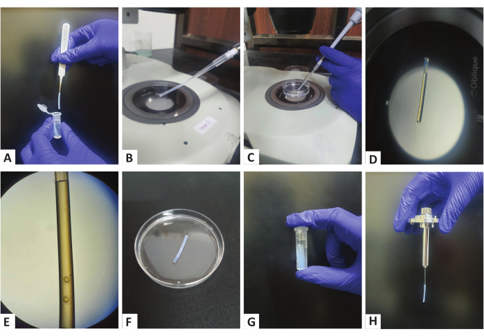
Figure 1: Sample preparation using polymer tubes. (A) A polymer tube from the stored microcentrifuge tubes is taken using forceps. (B) Attaching the tube to the tip of a 200 µL micropipette. (C) Aspirating embryos with the help of a pipette into the tube. (D,E) A polymer tube with bud-stage embryos visible towards the bottom of the tube. (F) The polymer tubes are placed on a Petri dish with E3 to solidify the agarose. (G) Storing the polymer tubes in a microcentrifuge tube filled with E3. (H) Assembled sample holder with the mounted polymer tube. Please click here to view a larger version of this figure.

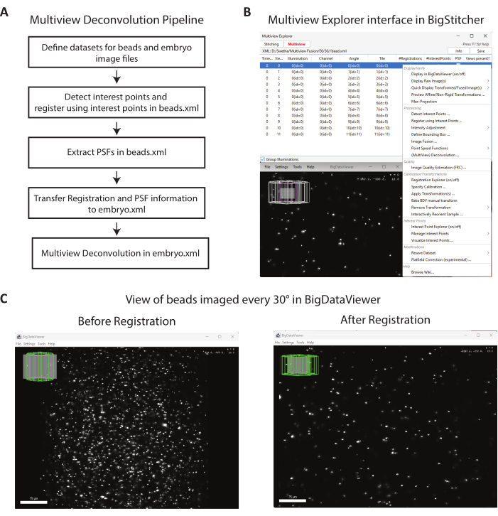
Figure 2: Multiview image analysis workflow and registration using beads. (A) The multiview image analysis pipeline. (B) The image shows the "Multiview Explorer" window in BigStitcher, a FIJI plugin, where each view appears as a single row and contains information about the angle, channel, registration, interest points, and PSF. All commands discussed in the protocol appear when a view is selected and followed by a right click, as depicted in the pop-up menu. The selected views can be visualized in the BigDataViewer window, as shown. (C) A representative bead image before (left) and after registration (right) obtained from imaging at 30° angular intervals. All angular views have been selected and displayed. Scale bars: 75 µm. Please click here to view a larger version of this figure.

Figure 3: Overview of default embryo orientations. Representative images of the orientations the embryos fall into within the chorion at 70% epiboly (A) and bud stages (B). The top row in each panel depicts bright-field images obtained from the light sheet system, and the bottom row depicts representative cartoons. Arrows in (B) indicate the position of the notochord, which was used for identifying the orientation. Ap, animal pole; Vp, vegetal pole; A, anterior; P, posterior. Scale bars: 100 µm. Please click here to view a larger version of this figure.

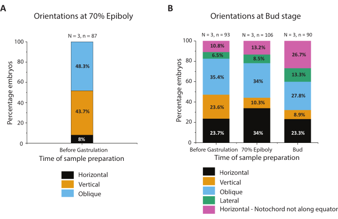
Figure 4: Statistics of different embryo orientations. (A) The stacked column indicates the percentages of embryos that fall into the indicated orientations at 70% epiboly when samples are prepared before gastrulation. (B) The stacked columns indicate the percentages of embryos that fall into the indicated orientations at bud stages when samples are prepared before gastrulation (left), at 70% epiboly (middle), and at bud stages (right). N, the number of independent clutches from which embryos were obtained; n, the total number of embryos. Please click here to view a larger version of this figure.

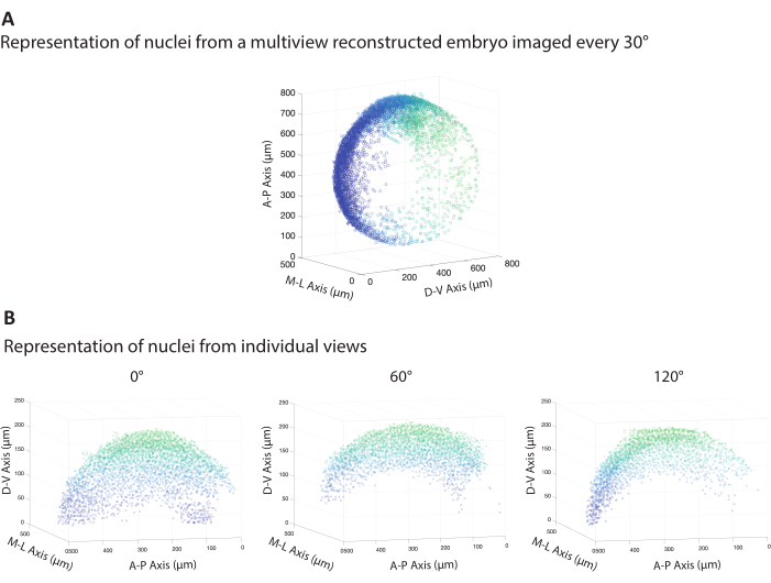
Figure 5: Representation of nuclei from a multiview reconstructed embryo. (A)The 3D scatter plot represents nuclei detected in a multiview-reconstructed embryo imaged at 30̛° angular interval. Each circle represents a nucleus and the centroid of nuclei positions are plotted. The nuclear coordinates were obtained using Mastodon, a FIJI plugin. (B) 3D scatter plots of nuclei from three representative views of the same embryo - the depictions being 60° apart. Colors for each nucleus were randomly assigned. Please click here to view a larger version of this figure.

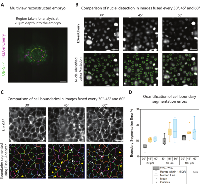
Figure 6: Comparison of cellular-scale information in fused images. (A) The image on the left shows a snapshot from a multiview-reconstructed embryo at a 20 µm depth from the surface. The yellow circle depicts the region used for further analysis. Scale bars: 50 µm (in all panels). (B) Representative raw images of nuclei at 20 µm depth from the surface of the embryo from three data sets imaged every 30°, 45°, and 60° respectively (top). Nuclei detected (in green) in the same images by Mastodon, a FIJI plugin (bottom). (C) Representative raw images at 20 µm depth from the surface of the embryo from three data sets imaged every 30°, 45°, and 60° respectively, using the actin marker, Utr-GFP (top). Boundaries segmented by Tissue Analyzer, a FIJI plugin, are shown for the same images (bottom). Arrows indicate errors made by the Tissue Analyzer in boundary segmentation, with the yellow arrow representing a missing boundary and the white arrow representing wrongly detected boundaries when visually no boundaries appear to exist. (D) The box plot depicts the percentage of errors the Tissue Analyzer made between multiview reconstructed embryos imaged every 30°, 45°, and 60° at different depths. Error bars indicate 1.5 times the interquartile range. Please click here to view a larger version of this figure.

Discussion

Positioning an embryo in the right orientation to image the region of interest is one of the rate-limiting steps that often results in a failed microscopy session for a user. This is more so in a multiview light sheet microscope where manual manipulation of the orientation is difficult as the samples are embedded within a tube. To aid in this process, this study reports the statistics of various positions a zebrafish embryo takes up between 70% epiboly and early somite stages within a chorion when the polymer tube with embryos is kept upright in a microcentrifuge tube.

At 70% epiboly, vertically or horizontally oriented embryos provide complementary information of events across the entire embryo. While the horizontal orientation allows visualization of cellular dynamics in the animal pole as well as the dynamics of cells undergoing epiboly as viewed from the vegetal pole, the vertical orientation allows for visualization of dorsal and ventral sides of the embryo, including cellular dynamics in the dorsal organizer, internalization of cells during gastrulation and convergence-extension flows. This study shows that there is a high probability of obtaining an embryo in the vertical orientation purely by chance if the samples are prepared a few hours prior to imaging; however, the horizontal orientation seems to be much less prevalent at these stages. For stages prior to 70% epiboly, it is recommended that users document similar statistics of embryo orientation within the chorion before proceeding with time-lapse imaging, as having this information beforehand saves time in the long run.

From the bud stage, the best orientation for imaging is a horizontally positioned embryo, as this allows following cellular dynamics along the entire anteroposterior body axis of embryos¹⁵. Getting an embryo in this orientation is relatively straightforward, as about 25% of the embryos fall into this stable position irrespective of when the sample is prepared. In general, for imaging any stage of interest, preparing about 15 tubes with two to three embryos in each tube is recommended, which will ensure a high probability of obtaining embryos in the desired orientation and, hence, a successful microscopy session on any given day. In addition, it is recommended that the tubes be sorted about an hour before the stage of interest to choose an embryo with the right orientation for time-lapse imaging.

After obtaining an embryo in the right orientation, it is important to factor in the number of views and the angle interval between the views for imaging. This depends on the minimum required spatial and temporal resolution. The more angles from which a particular structure or region of the embryo is imaged, the better the spatial resolution (as shown in Figure 6), but this leads to a compromise on the temporal resolution. In this protocol, with a system that has two illumination and one detection arms, imaging two channels over a full 360° with an angular interval of 30° and about 100 z-slices in each angle with a slice spacing of 2 µm, took about 3 min for one-time point. While this is sufficient to track cells in early embryonic stages, if events with faster dynamics are to be captured, a smaller number of angles have to be acquired, ensuring better temporal resolution but with a compromise on spatial resolution, especially if finer structures such as cell boundaries have to be segmented. A second option to consider to improve temporal resolution is to use a multiview system with two detection arms, which will substantially increase the acquisition speed as recently used for tracking cell movements during gastrulation in zebrafish embryos¹⁶. In addition, although only the 20x/1 NA objective was tested in this protocol, depending on the sample being imaged, the required spatial resolution, and the field of view, the right objective needs to be considered. Taken together, based on the required downstream processing and quantification for a particular sample and field of view, the number of views and the angle interval need to be carefully chosen. For imaging entire early zebrafish embryos, particularly with cellular-scale resolution from multiple angles, however, a 20x/1 NA objective seems to be optimal, as an objective with a lower magnification and NA (for e.g., 10x/0.5 NA objective) will have much lower resolution, likely leading to more segmentation errors, while an objective with higher magnification and NA will not be feasible for covering the entire embryo in the field of view of the camera.

In this study, to discuss mounting and imaging strategies, an actin marker, which can be used as a proxy for tracing cell boundaries, and a histone marker, for detecting and tracking nuclei, were used. In fact, most of the previously published studies that have used a multiview light sheet system have preferentially used similar markers^5,7,15,16,27. The main reason for choosing these markers is that multiview light sheet microscopy is majorly used for following cellular-scale dynamics (e.g., cell shape and cell rearrangement) either at tissue scales or across the entire embryo for long time periods spanning several hours to days. On the other hand, if there is a need for obtaining sub-cellular resolution, a different transgenic line marking the region of interest could be used, but in this scenario, a multiview light sheet microscope may not be the best choice of instrument, and rather a confocal, a super-resolution system or even a lattice light sheet microscope^28,29 may better suit the problem being investigated.

The discussed protocol works well from gastrulation to 15-somite stage zebrafish embryos³⁰ (about 17 hpf) without any modifications, and although not tested here, it is likely to work for earlier embryos before the gastrulation stage as well. Beyond the 15-somite stage, spontaneous muscle contractions begin^30,31, which can be suppressed by adding tricaine, an anesthetic, in the tube as well as in the sample chamber. In addition, at about 18 hpf, tail eversion away from the yolk begins³⁰, which moves the embryo away from the field of view. To take care of this, a tracking algorithm that tracks the elongating end needs to be employed to keep the embryo in focus³². Furthermore, for imaging later-stage embryos when they are devoid of a chorion, such as for following neural development, an alternate mounting strategy needs to be employed as recently performed³³.

For imaging zebrafish embryos with an intact chorion, capturing both the beads, which act as registration markers, and the embryo in the same field of view is not possible using a 20x/1 NA objective. This study provides a simple alternative by registering the different views with information from beads that are present above or below the sample, followed by shifting the registration from the beads to the embryo during processing. Once the embryo sample is registered this way, a second round of registration using nuclei as registration markers may be performed, which are present within the sample, for further fine-tuning the initial registration. When performing time-lapse imaging, the nuclei information, in turn, can be used for registration of consecutive time points as has been reported previously²¹. One alternative to this protocol is to forego beads and instead use the nuclei information for the initial registration. But the registration often failed (not shown here) in the BigStitcher plugin, possibly due to a combination of many nuclei not getting detected deeper in the embryo during processing and also because of a relatively smaller number of nuclei that are present in the embryo when viewed from certain angles (for example when viewed ventrally at late epiboly stages).

In this protocol, because bead information from above or below the sample is used for registration and there is no need for imaging beads in the same view as imaging the sample, one can use this protocol for imaging only specific regions of interest but at high magnification from different angles instead of the entire embryo. Furthermore, it is easy to adapt this protocol for imaging multiple samples stacked vertically in the tube by using bead information from between the samples for registration.

Materials

List of materials used in this article

Name	Company	Catalog Number	Comments
Agarose, low gelling temperature	Sigma-Aldrich	A9414
Calcium Chloride dihydrate	Sigma-Aldrich	12022
FIJI			Version: ImageJ 1.54f
Latex beads, carboxylate-modified polystyrene, fluorescent red, 0.5 μm mean particle size, aqueous suspension	Sigma-Aldrich	L3280
Magnesium sulfate heptahydrate	Sigma-Aldrich	M2773
mMESSAGE mMACHINE SP6 Transcription kit	ThermoFischer Scientific	AM1340	For in vitro transccription of H2A-mCherry plasmid
Potassium Chhloride	Sigma-Aldrich	P9541
Potassium phosphate monobasic	Sigma-Aldrich	P0662
PTFE Sleeving AWG 15L - 1.58 mm ID x 0.15 mm Wall +/-0.05	Adtech Innovations in Fluoroplastics	STW15	PTFE tubes
Sodium Chloride	Sigma-Aldrich	S3014
Sodium phosphate dibasic	Sigma-Aldrich	71640
Ultrasonic Cleaner	Labman	LMUC3	Ultrasonicator
Zeiss LightSheet 7 System	Zeiss