Software for Analysis of Heart Rate and Blood Pressure Time-series Data from the Valsalva Maneuver

Summary

The ValsalvaAnalyzer software includes functions to analyze continuous beat-to-beat electrocardiogram and blood pressure (BP) measurements recorded during the Valsalva maneuver (VM). The computed clinical biomarkers and estimated model outputs provide insight into sympathetic and parasympathetic regulation of heart rate and BP during the VM.

Abstract

The Valsalva Maneuver (VM) is a low-risk highly accessible test that measures the baroreflex-induced heart rate (HR) and blood pressure (BP) response to forced breathing against 40 mmHg intrathoracic pressure for 15 s. This study demonstrates the ValsalvaAnalyzer software, which combines modeling and data analysis to extract biomarkers from time-series BP and electrocardiogram (ECG) data. The software, programmed in MATLAB, incorporates a graphic user interface, making data analysis and mathematical modeling predictions accessible to clinicians. The software calibrated for PCs and Macs reads ECG and BP data measured during the VM. It automatically identifies R and S peaks in the ECG signal, with integrated user verification to ensure the accuracy of the captured signals. The RR intervals are used to predict HR, and the QRS complex magnitude changes are used to predict respiration. Systolic and diastolic BP are captured, and the user identifies the onset and VM duration from the SBP. The software automatically detects the four VM phases and the intrathoracic pressure. The latter is obtained by merging the respiratory signal at rest with the 40 mmHg pressure the subject breathes against during the VM. The most commonly reported clinical VM markers computed from the HR and BP data are reported along with estimates of patient-specific parameters obtained using a differential equations model, which predicts sympathetic and parasympathetic dynamics. The final output, over 35 metrics, includes BP and HR, maximum and minimum HR, the Valsalva ratio, and measures of baroreflex sensitivity, all saved to a spreadsheet. The software is intended to analyze the VM data, but the methodology can be extended to other autonomic tests. Its strength lies in combining quantities extracted from raw data with model outputs, augmenting clinical data with a mathematical model providing insight into autonomic immeasurable quantities.

Introduction

The Valsalva Maneuver is a low-risk, non-invasive, inexpensive, and highly accessible test to measure the autonomic nervous system function through forced expiratory exercises^1,2. The maneuver is performed by patients exhaling into a positive end-expiratory pressure (PEP) device connected to a manometer, holding an intrathoracic pressure of 40 mmHg for 15 s, typically in a supine or seated position^2,3. This maneuver simultaneously challenges the autonomic and cardiovascular systems, mimicking the physiological response to stressors like straining while lifting heavy objects or equilibrating pressure when flying⁴. This test is used frequently in clinical settings^2,5, but more tools are needed to analyze data quantifying the underlying physiological mechanisms. Neurological modeling applied to the VM may facilitate the identification of improved diagnostic criteria and causal mechanisms for autonomic dysfunction⁵.

The VM has four phases⁶. It is facilitated by a breath hold, which increases intrathoracic pressure, compressing the cardiac chambers and the thoracic aorta and emptying blood in the systematic circulation, thereby causing a transitory increase in BP. Phase I is characterized by a continuous increase in intrathoracic pressure, reducing the venous blood flow to the heart, the stroke volume, and the mean arterial BP. In response, the high-pressure arterial baroreceptors are activated. The decrease in BP during the early part of Phase II causes a parasympathetic withdrawal, increasing HR. During the late part of Phase II, sympathetic excess mediates vasoconstriction, increasing BP and HR. In healthy patients, BP recovery is the resting value before releasing the breath hold. Phase III is reciprocal to Phase I. This phase is initiated when the patient releases their breath hold, which causes sharp decreases in intrathoracic pressure and arterial BP, usually followed by an HR increase. In Phase IV, increased venous return to the heart and persisting vasoconstriction from late Phase II results in a marked BP increase called an overshoot. Stimulation of high-pressure arterial baroreceptors by the overshoot activates the vagal nerve to reduce HR. The patient is expected to recover to pretest values approximately 10-30 s after the VM onset^2,5.

The VM is used for bedside evaluation of autonomic and cardiovascular function⁷. The most common VM biomarker, the Valsalva ratio (VR)^8,9,10, measures parasympathetic function as the ratio between the longest RR interval after the breath-hold onset and the shortest RR interval. It has previously been established that postural orthostatic tachycardia (POTS) is associated with a high VR and a notable BP overshoot in Phase IV¹¹, also called N-pattern response¹. Another metric is the vagal baroreflex sensitivity. This metric is estimated in the early part of Phases II and IV as the regression slope between RR intervals and characteristic BP changes^{3,10,12,13,14}. Qualitative analysis of BP responses to the VM can identify different heart murmurs⁹, and a distinctive square-wave response is a bedside indicator of impaired ventricular function and heart failure^15,16. The absence of BP overshoot and the presence of bradycardia after breath-hold release is indicative of dysautonomia¹³. The V-pattern response with progressive BP decline in late Phase II and slow recovery in Phase IV is characteristic of neurogenic orthostatic hypotension, indicating alpha-adrenergic baroreflex failure¹. Other studies have demonstrated the efficacy of using the VM to supplement head-up tilt testing in screening for orthostatic disorders^1,17,18.

Numerous studies have examined autonomic function by analyzing HR and BP responses during the VM¹, but no open-source automated systems are available to quantify the baroreflex function. Many studies have analyzed data from the VM^19,20,21,22, and a few software specialize in autonomic function, including VitalScan by Medeia²³ and Kubios²⁴. VitalScan utilizes ECG and BP signals, but Kubios only analyzes ECG signals. The VitalScan website notes that this software assesses autonomic function but lacks a detailed description of calculated quantities. Kubios determines HR variability (HRV) and the VR²⁵. To address these gaps, this study develops a new open-source software that calculates the most common VM indices^1,25.

The software analyzes ECG and BP data measured during a VM maneuver holding an intrathoracic pressure of 40 mmHg for 15 s. We recommend including at least 30 s stable data before and after the VM. After identifying HR and systolic BP, the VM onset and release, a set of clinical markers are extracted. In addition, this software uses the mathematical model by Randall et al.²⁰ to predict sympathetic and parasympathetic signaling along with parameters characterizing the baroreflex sensitivity. Two critical features are the ability to read data from noisy signals, to identify and remove artifacts, and the automatic detection with manual correction of VM markers. The latter is vital for patients with autonomic dysfunction, where purely automatic detection fails. This exposition includes all results for subject 1 and a protocol to extract results for subjects 2-8. Results for subject 1 is included in the code, text, and figures, and results for all subjects are shown in Supplementary Figure 1, Supplementary Figure 2, Supplementary Figure 3, Supplementary Figure 4, Supplementary Figure 5, Supplementary Figure 6, Supplementary Figure 7, and Supplementary Figure 8.

The Valsalva Analyzer software calculates adrenergic and vagal indices characterizing the response to the Valsalva maneuver (VM) from continuous ECG and BP measurements. To demonstrate the software, we provide a brief description of the experimental setup followed by a detailed description of the software. The software reads data extracted from patient records stored in LabChart. The analysis is demonstrated on a healthy control patient, but the software includes data from eight subjects with a range of autonomic responses. Below, we discuss patient examples and describe the protocol to install and run the software. The protocol includes references to figures generated within MATLAB. To distinguish these from figures included in the representative results, these are all referred to as MFigure #.

Protocol

Three example datasets were selected from adult male (age 30-45) blood donors eligible for blood donation according to the Danish legislation²⁶, three from a study examining the effects of preoperative opioids on adult (age 40-61) patients receiving knee and hip replacements²⁷, and one from a patient diagnosed with postural orthostatic tachycardia syndrome (POTS)²⁸. The BD and opioid studies were approved by the local ethics committee in Denmark (H-19069845 and H-20071567, respectively), registered with the Danish data protection agency, and registered at ClinicalTrials.gov (NCT04499664 and NCT04902222, respectively). Frederiksberg and Bispebjerg Hospitals, Denmark ethics committee approved using data to diagnose POTS for research. All data were deidentified before being prepared as examples for this software, and all subjects could speak and understand Danish and gave informed consent to participate in their respective studies.

NOTE: The software provides tools to extract markers from patient measurements of ECG and BP. Users can enter a subject ID number, age, sex, weight, and height. This information is optional. Users are encouraged to cite this manuscript. The software includes example data from measurements of ECG (channel 1), HR derived from ECG (channel 2), and BP (channel 3). Table 1 includes a detailed patient description and patient notes. The eight example deidentified data sets provided with this software were extracted from previously published studies^26,27,28. Data were selected to demonstrate characteristic features observed during the VM. The intention is to demonstrate the software's features, not to conduct a specific clinical study. Exclusion criteria for the blood donor and opioid studies include alcohol and drug abuse, and habitual use of opioids, arrhythmia or heart failure, history of orthostatic hypotension. Exclusion criteria not explicitly listed for each study are listed in^26,27.

Patient	Age (years)	Sex (m/f)	Height (cm)	Weight (kg)	BMI (kg/m2)	Notes
Subject 1	35	m	176	92	29.7 (ob)	Normal response
Subject 2	31	m	180	70	21.6 (nw)	Normal response
Subject 3	30	m	187	93	26.6 (ow)	Large overshoot in phase IV. HR artefacts due to ECG signal noise
Subject 4	42	m	175	76	24.5 (nw)	V-response typical for autonomic dysfunction. Inadequate chronotropic effect in phase II. No BP recovery in late phase II. Missing overshoot in phase IV.  Long PRT
Subject 5	37	f	165	85	31.2 (ob)	No overshoot in phase IV
Subject 6	61	f	170	107	37.0 (ob)	Inadequate BP recovery in late phase II. Maximal BP does not equal end BP in late phase II
Subject 7	42	m	177	84	26.8 (ow)	Missing overshoot in phase IV
Subject 8	58	f	166	77	27.9 (ow)	Negligible BP drop in early phase II. HR artefacts due to ECG signal noise. BP artefacts in phase IV
nw: normal weight BMI (18.5-25), ow: over-weight (BMI (25-30), ob: obese (BMI > 30)26

Table 1. Please click here to download this Table.

1. Experimental setup

1. Collect continuous measurements of BP from a finger blood pressure cuff placed on the index and middle fingers on the non-dominant hand (Figure 1A). Position the hand at the heart's level to eliminate gravity's effects (Figure 1B).
2. Measure ECG using a standard 3-electrode ECG with electrodes placed at equidistance from the heart at the left and right atrium and on the left side lower edge of the rib cage. After instrumentation, perform the Valsalva maneuver by the subject exhaling into a positive end-expiratory pressure (PEP) device connected to a manometer (Figure 1C,D).
3. Ask the subject to breathe normally for 1-5 min until a stable signal is generated. To have sufficient data for analysis, record stable signals for at least 30 s before and after the VM. Perform VM by asking the subject to exhale for 15 s, holding a pressure of 40 mmHg (Figure 1D). During the recording, if possible, turn calibration off to avoid gaps in BP signal.
4. The software analyzes signals exported from LabChart to MATLAB at 1,000 Hz. In the Export as MATLAB menu, include channels with ECG, HR, and BP signals, and intrathoracic pressure if recorded. Note the channel numbers for each signal. In the menu, choose 32-bit floating pint, Upsample to same rate, uncomment Comments and Event markers. Click OK to export .mat file and Cancel to stop the export.

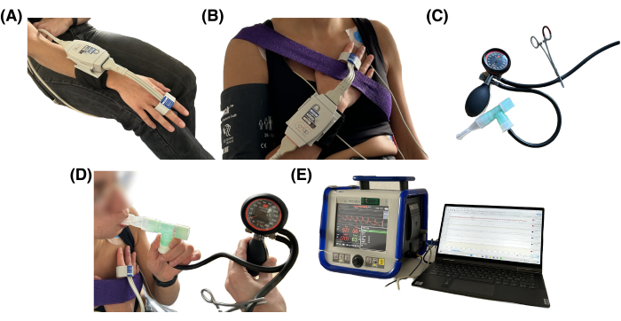
Figure 1: Instrumentation, BP cuff, ECG placement, monitor, VM equipment. (A) Mounting of the BP cuff on the index and middle finger on the non-dominant hand. (B) The finger BP cuffs are fastened at the level of the heart, using a cohesive CoFlex bandage to eliminate the effects of gravity. (C) PEP device attached to a manometer. (D) The seated subject exhales into a positive end-expiratory pressure (PEP) device connected to a manometer, holding an intrathoracic pressure of 40 mmHg for 15 seconds. (E) The CNAP module continuously measures BP and is connected to a computer that processes and saves data using LabChart. Please click here to view a larger version of this figure.

2. Software installation, data upload, and startup

NOTE: This protocol describes how to export signals from LabChart to MATLAB, but the protocol does not depend on recordings stored in this software. We refer to their manuals for signals recorded by other software and note that conversion may be needed to export recordings in the correct format. Data must include continuous time-series measurements of ECG and BP.

1. Download the ValsalvaAnalyzer Software. Clone the GitHub Repository at https://github.com/msolufse/ValsalvaAnalyzer. Click the green Code button. Click Download ZIP.
2. Navigate to the folder ValsalvaAnalyzer. The main script DriverBasic.m should be replaced by the ValsalvaAnalyzer folder, and all other scripts (.m files) should be in the Core folder. The software includes subfolders: Figures, Markers, Optimized, Sensitivities, and WS.
   NOTE: The folder Figures stores generated figures. This folder contains two subfolders (Data and Model_fits): Data stores for figures generated from the data analysis and figures generated by the differential equations model. The Labchart folder includes the exported .mat files but not the original LabChart files. The folder Markers hold the spreadsheets with clinical ratios (one file per subject). The Sensitivities and Optimized folders include .mat files with the sensitivities and estimated parameter values. The folder WS contains .mat files generated when cleaning data. The main folder ValsalvaAnalyzer includes DriverBasic.m, the core script needed to run the program. When the software is downloaded. The folder Labchart includes a .mat files for each of the eight example subjects, while the folders with results (Markers, Sensitivities, Optimized, and WS) only have results for Subject 1. As the example datasets in the folder are analyzed, output files will be stored in these folders. The file Patientinfo.xls (and Table 1) includes patient information (age (years), sex (m/f), height (cm), weight (kg), and BMI (kg/m²)) for each of the eight example datasets. The weight is characterized as normal (nw), overweight (ow) or obese (ob)²⁹, and it is noted if the subject has a normal or pathological VM response.
3. To run the software, go to the folder ValsalvaAnalyzer and open the file DriverBasic.m in MATLAB. In the top panel, click Editor, and then click the Green triangle labeled Run to execute the program.

3. Software platform

NOTE: The software distributed by GitHub has been tested on Windows (Windows 11 Education) and Mac (MacOS Sonoma, version 14.3) and uses MATLAB (version R2023a). Defaults are set to the MacOS environment with suggestions for Windows.

1. From the pop-up menu Select Figure Parameters, select the software platform type, the figure font size, marker size, and linewidth.
2. Click OK to accept and proceed to Step 4 or click Cancel to end the program.

4. Patient selection

NOTE: This step involves the selection and analysis of data. The software will read .mat files from the Labchart folder.

1. Select any number of patients from the list using the mouse. The button Select all marks all patients. Patient labels are determined from the filenames. These are used in all exported files. Click OK to proceed to Step 5 or Cancel to exit the program.

5. Selection of operation

NOTE: The data analysis methods are listed in a menu providing available operations. These include methods for cleaning ECG and BP data, identifying VM phases, and computing VM features. The former is carried out on the raw data using the sampling rate embedded in the measurements (the attached examples are sampled at 1,000 Hz). The identification VM features use cleaned HR and systolic SBP signals subsampled at 10 Hz. The subsampled data are also used to determine sympathetic and parasympathetic signaling obtained from solving the differential equations model by Randall et al.²⁰ Generated figures are saved as .png files and stored in the Figures folder and generated numbers are stored in a spreadsheet (.xlsx) in the Markers folder. The layout of the functions within this software is illustrated in Figure 2.

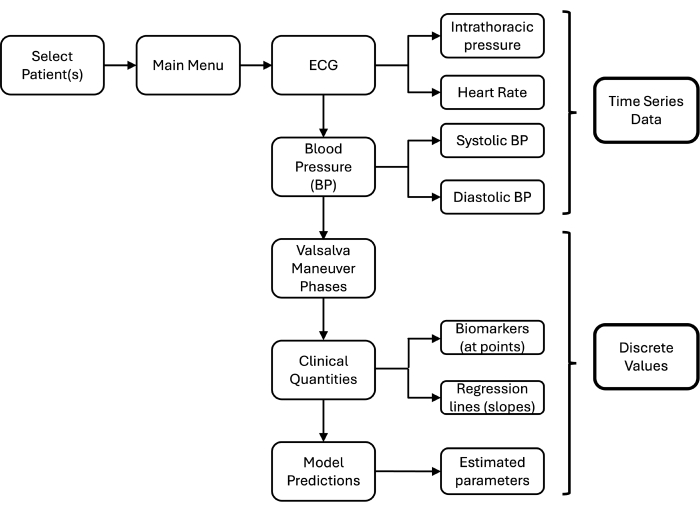
Figure 2: Software operations. After selecting patients, the software provides the option to correct measured signals, including (1) the ECG, from which heart rate and respiration are extracted, (2) the beat-to-beat blood pressure (BP) signal from which systolic and diastolic BP are extracted. After these procedures, the software identifies the Valsalva maneuver phases and extracts clinical biomarkers. Finally, we provide the option of running a computational model predicting baroreflex function. Please click here to view a larger version of this figure.

1. Select operation(s) to be performed in the Subset selection menu. Complete operations in descending order, e.g., patient information should be inputted before the ECG is analyzed. If more than one subject and task is selected from the Operation Selection menu in step 4, the software will complete the first task for all subjects before moving to the next task.
   1. The software includes the following operations: Patient Information (Operation 1, Step 6); Electrocardiogram (ECG; Operation 2, Step 7); Heart Rate (HR; Operation 3, Step 8); Respiration (Operation 4, Step 9); Blood Pressure (BP; Operation 5, Step 10); VM Phases (Operation 6, Step 11); Clinical Ratios (Operation 7, Step 12); Model Prediction (Nominal; Operation 8, Step 13); Sensitivity Analysis (Operation 9, Step 14); Optimization (Operation 10, Step 15); Plot Model Predictions (Operation 11, Step 16); Summary (Operation 12, Step 17).
2. After selecting operations, Click OK to proceed to the operation or click Cancel to return to Step 4.

6. Patient information (Operation 1)

NOTE: The first operation involves inputting patient characteristics (ID, Age, Sex, Height, and Weight) the channel numbers from the exported Labchart  file (ECG, HR, BP, intrathoracic pressure - if available), and identifying the time range for the data analysis.

1. Enter patient ID (integer), Age (integer, years), Sex (m/f, male/female), Height (real number, cm), and Weight (real number, kg). Click OK to proceed or Cancel to return to Step 5. The software will run without selections. Characteristic values for the eight subjects are listed in Table 1. These values are not used in the data analysis but may be helpful for summary statistics.
2. Identify in what channel each signal is stored, default values are: Channel 1 (ECG), channel 2 (HR),  channel 3 (BP), channel 4 (intrathoracic pressure - Pth) is set to 0. The example datasets 1-8 does not include this signal.
3. MFigure 1 (Figure 3) displays the ECG (mV) top, HR (bpm) center, and BP (mmHg) bottom as functions of time (seconds). Select data to analyze. Include approximately 20 s before and after the VM.
4. Positioning the crosshair, click once with the mouse at the start (~20 s before the VM) and a second time at the end (~20 s after the VM). The selected data will appear in red in MFigure 1. Click Save and Exit. MFigure 1, with the selected data, will be saved in the folder Figures/Data under the name [patient name] + _dataAnalyzed.png.

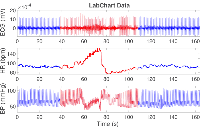
Figure 3: Graphs depict the ECG (mV, top), heart rate (HR bpm, center), and blood pressure (mmHg, bottom) data. The blue trace shows all data extracted from LabChart, and the red trace shows data selected for analysis in this study. The red region containing ECG, HR, and BP starting and ending ~20 sec before and after the VM maneuver. Please click here to view a larger version of this figure.

7. Electrocardiogram (Operation 2)

NOTE: Operation 2 involves identifying R and Q or S peaks in the ECG signal (removing extra and/or adding missing peaks). This operation is performed on the raw data sampled at 1,000 Hz. The magnitude of the QRS complex (the absolute distance between the R and Q or S peaks) is used to create the respiration signal before and after the breath hold.

1. MFigure 1 displays the ECG signal (black line). Automatically detected R peaks are marked with red and Q or S peaks with blue circles. The objective is to correct misplaced peaks. The total number of R and Q or S peaks is printed to the right of the graph. This task can only be completed if the number of R and S peaks are the same. To correct the misplaced peaks, scroll with the hand to the right through the signal and stop when the peaks to be corrected are in the window. An example of an extra wrongly placed S peak and the signal after the peak has been removed is shown in Figure 4.
   NOTE: The R and S peaks are identified using the methodology described by Randall et al.²⁰. This algorithm uses findpeaks.m to find peaks between 25% to 200% of the mean signal. The sampling rate is 1,000 Hz (encoded in the data), and the MinPeakDistance is set to 1.5. R peaks are found from the raw signal, and S (or Q) peaks are found by analyzing the negative of the signal. It should be noted that for some datasets, the algorithm will identify S peaks and for some Q peaks. Examples are shown in Figure 4A. The QRS magnitude is used to determine respiration as described by Randell et al.²⁰.
2. Repeat correction until the number of S and R peaks are the same using the steps described below.
   1. To correct the misplaced peaks, scroll to the right and stop when the peak(s) to be corrected are in the window.
   2. If a peak is missing, placed wrongly, or an extra peak is marked, scroll to the location of the peak. Press Enter on the keyboard, and a crosshair appears. Click on the point to correct. The next menu query is: Add or remove point? Select either Add (step 7.2.3), Remove (step 7.2.4), or Cancel, returning to Step 7.2.1.
   3. Click Add, and the point marked will be added and appear in red (R peak) or blue (Speak). The program will use the exact location of the click and automatically classify the point as R or S.
   4. Click Remove, and the point marked will be removed. Repeat this step if the point does not disappear, returning to task 7.2.2.
3. Repeat step 7.2 until all R and S peaks are identified correctly and the number of R and S (or Q) peaks are the same. Then press Enter on the keyboard. On the prompt asking to correct points, click No. Continue with operation 3 (HR). If the time series has no errors, but the number of R and S (or Q) peaks is not identical. To correct this error, return to Step 7.2. Note that for consistency within a signal, choose either S or Q peaks.
4. If the user clicks No when the number of R and S peaks is not identical, a new menu pops up, noting that the Number of R and S peaks must be equal. Inspect data. Click OK and the code returns to Step 7.2.

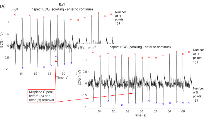
Figure 4: Graphs used to guide ECG (mV) correction. The figure shows the ECG trace (black), R waves (red circles), and S waves (blue circles). (A) The graph has a misplaced S wave. In (B), this S-wave has been removed. A clean ECG signal will have the same number of R and S peaks, as noted on the right side of the graph. Please click here to view a larger version of this figure.

8. HR (Operation 3)

NOTE: This step involves converting the RR intervals to HR. After the ECG signal has been corrected (as described above), for most datasets, the HR signal is smooth. However, if the HR signal has artifacts (example shown in Figure 5A). Operation 3 provides the opportunity to correct the signal (example shown in Figure 5B).

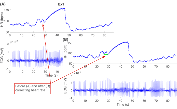
Figure 5: Graphs used to guide heart rate (HR, bpm) correction. (A) Heart rate (blue line) generated from the corrected ECG. The small blue circles mark the times at which the heart beats. (B) Example of a spline connecting two points (green line), removing an artifact from the heart rate signal. Please click here to view a larger version of this figure.

1. MFigure 1 (Figure 5A) displays HR (bpm) in the top panel and ECG (mV) in the bottom panel. The HR (bpm) is computed from the corrected ECG RR peaks. If the HR signal does not have artifacts, click Save and Exit, and continue to Operation 4 (Respiration). If there are errors in the data (compare the two panels in Figure 5), click Correct Heart Rate and proceed to Step 8.2.
2. Scroll along the HR signal and locate artifacts. Press Enter on the keyboard when viewing a region to correct. Proceed to Step 8.3.
3. Click OK on the menu querying Click at points to connect. Align the crosshair over the first point before the artifact and click once with the mouse. Then, align the crosshair over the first point after the artifact and click a second time with the mouse. A linear spline (plotted in green) connects the two points. A menu asks, Accept change? Answers: Yes (proceed to Step 8.3.1), Undo (go to Step 8.3.2), and Add change (go to Step 8.3.3).
   1. Select Yes to accept the linear spline, exit this operation, and return to Step 4. Select Undo to remove the linear spline and return to Step 8.2. Select Add to keep the linear spline and return to Step 8.2 to allow additional corrections.
4. MFigure 1 displays the HR (bpm) and ECG (mV) in the top and bottom panels. The figure is saved in the folder Figures/Data under the name [patient name] + _HeartRateECG.png. To continue, press Save and exit. The signals will be stored at the sample rate (1,000 Hz for the example datasets) embedded in the measurements.

9. Respiration (Operation 4)

NOTE: A respiration signal is extracted from the corrected ECG signal by computing the QRS complex magnitude, fitting a piecewise cubic Hermite interpolating polynomial spline (using interp1.m with the pchip method) through this difference as described in the study by Randall et al.²⁰.

1. MFigure 1 (Figure 6) depicts the respiratory signal extracted from the difference between the corrected R and S peaks. Inspect the graph, click Save and exit, and continue to operation 5 (blood pressure). MFigure 1 will be saved in the folder Figures/Data under the name [patient name] + _RespiratorySignal.png.

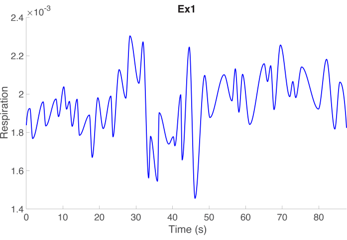
Figure 6: Respiratory signal. Respiratory signal (blue line) generated from the QRS interval amplitude changes, as described by Randall et al.²⁰. Please click here to view a larger version of this figure.

10. Blood Pressure (Operation 5)

NOTE: This step involves extracting systolic and diastolic BP. Two curves are formed by generating a spline through selected data points. For this operation, the user can correct the automatically detected curves. Given the significant change in BP, correction is likely needed immediately following the breath hold release.

1. MFigure 1 (shown in Figure 7A) displays a zoomed window with the BP data. Align the crosshair with a BP peak and click once with the mouse. Then, align the crosshair on the next peak to the right and click again. The distance between the two peaks estimates the cardiac cycle length. This distance is needed to identify systolic and diastolic peaks. MFigure 2 (Figure 7B,C) appears, displaying automatically detected systolic and diastolic signals.
   NOTE: The systolic and diastolic peaks are found using peaks2.m, which inputs the length of the cardiac cycle at rest to set the minimum peak distance. Similar to R. The systolic peaks are found directly from the signal, and diastolic peaks are found by analyzing the negative signal.
2. Systolic BP correction: A menu appears, prompting: Do you want to correct systolic points? Press Yes (Step 10.4) to initiate a protocol for fixing the systolic BP and No (Step 10.3) to proceed to correct the diastolic BP.
3. Diastolic BP correction starts with a menu asking: Do you want to correct diastolic points? Press Yes (Step 10.4) to initiate a protocol for fixing the diastolic BP and No to proceed. Press Save and exit and continue with operation 6 (Valsalva maneuver phases).
   NOTE: The protocol for correcting diastolic BP is identical to the one correcting systolic BP; both are described in Step 10.4.
4. MFigure 2 shows a zoom of the first 40 s data. Inspect the region and keep scrolling until a wrong point appears (corrected trace shown in Figure 7B,C). Press Enter on the keyboard and place the cross-hair on the last correct peak before the misplaced point(s), click on this point, and continue moving the cross-hair, clicking on all points to be corrected, ending with a correct point. Press Enter when finished. A dashed line appears connecting the corrected points (examples shown in Figure 7B,C).
   ​NOTE: Correction can be repeated until no more segments need to be modified. For each section, the corrected points are connected with a red (SBP) and green (DBP) dashed line attached to existing points at each end. The continuous BP signal, plotted in blue, is used as a guide. The system will record peaks clicked even if they do not align with the BP signal. This operation corrects the systolic and diastolic signals. Within each signal, only correct points associated with the signal, i.e., do not try to correct diastolic points when correcting the systolic BP or vice versa.

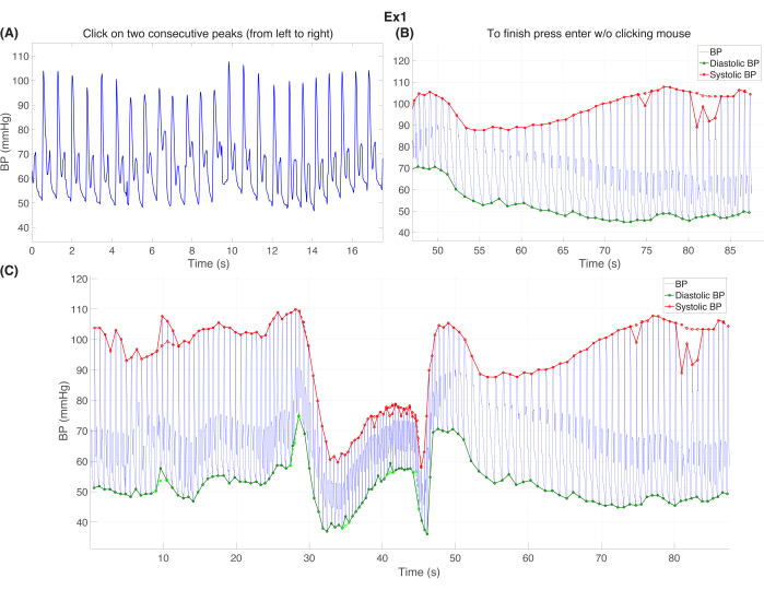
Figure 7: Blood pressure correction. (A) Zoom of the BP signal at rest. The user is asked to click on two consecutive peaks to determine the average length of the cardiac cycle. (B) A zoom of the original and corrected systolic (red) and diastolic (green) pressure. In this panel, the continuous blood pressure measurements (mmHg) are shown in blue. (C) The original and corrected systolic (red) and diastolic (green) blood pressure signals over the time range analyzed. In all panels, the continuous beat-to-beat BP signal is shown with a blue line, the SBP with a red line, and the DBP with a green line. For the SBP and DBP signals, each cardiac cycle is marked by small stars. Please click here to view a larger version of this figure.

11. Valsalva Maneuver (VM) Phases (Operation 6)

NOTE: Operation 6 involves the detection of the VM. This operation uses HR, SBP, DBP, and the intrathoracic pressure (if available) data subsampled to 10 Hz. The user is asked to identify the onset and release of the breath hold. The breath hold starts at the lowest BP value before the first peak and is released at the BP value before the second BP drop. After identifying these points, the software determines the four VM phases from the characteristics of the signals. These can be corrected manually, which is especially important when analyzing data for abnormal hemodynamic responses.

1. MFigure 1 depicts the continuous (thin line) and systolic (SBP, bold line) BP in the top panel (mmHg), HR (bpm) in the 2^nd panel, respiration (Resp, mV) in the 3^rd panel, and ECG (mV) in the bottom panel If intrathoracic pressure is available, this signal will be shown in the 3rd panel (Pth, mmHg), and the respiratory signal  (Resp, mV) in the 4th panel. The Valsalva phases are automatically detected, and the software continues to step 1.3  for datasets without Pth measurements. To mark the VM start, align the crosshair with the breath-hold onset (the SBP minimum immediately before the significant SBP rise and HR decrease) and click once with the mouse.
2. To mark the VM end, align the crosshair with the breath-hold end (the BP value immediately before the 2^nd SBP drop) and click once with the mouse. These points are used to determine the four VM phases in MFigure 2, displaying BP (mmHg) in the top panel, HR (bpm) in the center panel, and respiration (Resp, mV) in the bottom panel. If the intrathoracic pressure (mmHg) is measured it is shown between the heart rate and respiration panels.
3. A menu queries: Accept indices? Select Yes to complete the operation and continue to Operation 7 (clinical ratios). Select No to inspect the automated detection of phases delineated by vertical lines.
4. A menu queries: Index Correction. Select one, multiple, or all phases, then click OK to proceed to Step 10.4 for correction or Cancel to return to Step 11.1.
5. A crosshair appears in MFigure 2. The second line of the title describes the phase being corrected. For the selected phase, click the time, marking the onset of the phase. Repeat this operation until all selected phases have been corrected. The corrected times are shown with red vertical lines. Once all selected phases have been corrected, the menu reappears, querying: Accept indices? Clicking Yes continues to Step 11.5, and No reverts to Step 11.1. Note that the phases must be corrected in sequential order.
6. MFigure 3 (Figure 8) displays the final VM phases. The figure shows BP (mmHg) top panel, HR (bpm) center panel, and thoracic pressure (Pth, mmHg) bottom panel. This signal is obtained by merging the extracted respiratory signal with the measured or computed intrathoracic pressure enforced during the breath-hold. The four phases are shaded in gray. Click Save and exit and continue to operation 7 (Clinical ratios). This figure will be saved in the folder Figures/Data under the name [patient name] + _VMphases.png.

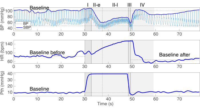
Figure 8: Valsalva Phases I-IV. The top graph shows continuous (light blue) and systolic (thick blue line) blood pressure; the second panel shows heart rate, and the bottom panel shows thoracic pressure. The latter is obtained by merging the respiratory signal with pressure during breath-hold (set to 40 mmHg). The Valsalva Phases I and III are marked with gray panels. Baseline values (mean SBP, HR before and after the VM) are denoted by horizontal dashed lines. Please click here to view a larger version of this figure.

12. Clinical ratios (Operation 7)

NOTE: This step computes clinical ratios characterizing the VM using HR, RR, and SBP, data subsampled to 10 Hz. All factors are listed in Table 2. These include patient characteristics (patient ID, age, sex, height, and weight), duration of the VM phases, minimum and maximum BP, HR, RR intervals within each VM phase^30,31, and pressure recovery time^32,33. The slope and goodness of fit (R² value) of the HR and RR regression lines in early Phase II (cyan line) and IV (brown line), characterizing vagal stimulation and pressure increase in early (cyan line) and late (blue line) Phase II and early Phase IV (brown line). The latter determines sympathetic stimulation. In addition, the software characterizes the change in SBP, vagal^1,32,34,35, and adrenergic (BRS)^1,32,33,36 markers. Again, the automatically detected phases and points can be corrected as needed. For example, the maximum BP and minimum HR in early Phase IV are often misaligned. Figure 9 depicts the clinical ratios before (panel Figure 9A) and after (panel Figure 9B) correction. Figure 9C depicts the ratios adapted from Palamarchuk et al.¹ and Sandroni et al.³¹. Note quantities displayed in this figure are derived from the values extracted from the data described in Steps 12.1-12.4.

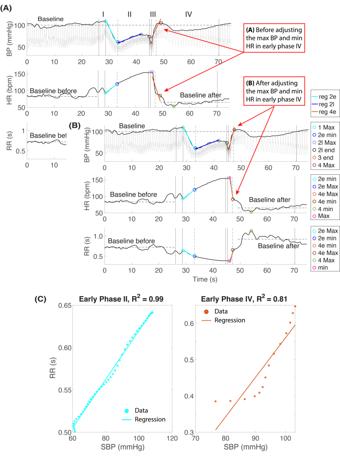
Figure 9: Clinical ratios. (A, B) Ratios and regression lines for blood pressure (BP, mmHg) in the top panel, heart rate (HR, bpm) in the center panel, and RR intervals (s) in the bottom panel. (A) shows the automatically detected ratios and panel (B) the corrected maximum BP and minimum HR in early Phase IV. (C) Regression line through corrected ratios. Please click here to view a larger version of this figure.

1. MFigure 1 (shown in Figure 9) depicts systolic BP (SBP, mmHg) in the top panel, HR (bpm) in the center panel, and the RR interval (s) in the bottom panel. Characteristic SBP, HR, and RR values are annotated with circular markers. A menu appears, querying: Do you want to accept markers? Inspect the markers. Click Yes if all points are correct; this operation is completed, reverting to Step 4. Click No if a point needs to be adjusted.
2. A menu queries: Select points to move. The menu enables the selection of one, multiple, or all points. If indices have been selected, click OK to continue (Step 12.3) or Cancel to proceed without changing any indices, continuing to Step 12.4.
3. For each selected quantity, a pop-up menu lists the points to be corrected. Click OK to continue. Align the crosshair at the desired point and click once with the mouse. When all selected points have been corrected, MFigure 1 displays BP (mmHg) in the top panel, HR (bpm) in the center panel, and RR intervals (s) in the bottom panel. It shows the corrected points and regression lines during early and late Phase II and early Phase IV. Press Save and continue to operation 8 (Run model).
4. MFigure 2 (shown in Figure 9C) displays the regression lines relating the RR interval to the SBP and the goodness of fit (the R² value). Press Save and exit, returning to Step 4. MFigures 1 and 2 will be saved in the folder Figures/Data under the names [patient name] + ratios.png and [patient name] + _ratios_regression.png.

13. Run model (Operation 8)

NOTE: Operation 8 involves solving the baroreflex differential equations model from Randall et al.²⁰, which predicts sympathetic and parasympathetic signaling. This step runs the model with parameter values set using patient information and clinical ratios identified in Operation 7. This operation is needed to test nominal predictions; if nominal fits have significant errors, results from the optimization operation (Step 15) may not be successful for the specific dataset.

1. Solves the differential equations model by Randell et al.²⁰ using nominal patient-specific parameter values extracted from the data and the patient information entered in Step 5. MFigure 1 depicts BP (mmHg) top left panel, HR (bpm) data (blue) and model (magenta) top right panel, thoracic pressure (Pth, mmHg) bottom left panel, and parasympathetic (magenta) and sympathetic (dark purple) predictions bottom right panel. The results are depicted with a time resolution of 10 Hz, which corresponds to the resolution in the subsampled HR and SBP data. Click Save and exit and continue to operation 8 (Run model). This figure will be saved in the folder Figures/Model_fits as [patient name] + _nominal.png.

14. Sensitivity analysis (Operation 9)

NOTE: Sensitivity analysis is not required for data analysis. This analysis generates a graph depicting model parameters' sensitivity (or importance) for accurate HR prediction. Sensitivities are evaluated at a frequency of 10 Hz, corresponding to the subsampled HR and SBP data. The operation uses local sensitivity analysis described in detail by Randall et al.²⁰

1. This operation computes the sensitivity of model parameters to HR. Results (on a log scale) depicting ranked sensitivities are shown in MFigure 1 (Figure 10). Click Save and exit, and continue to operation 10 (Optimization). Note that this computation takes a few minutes. The result shown in MFigure 1 is saved in the folder Figures/Model_fits as [patient name] + _sensitivities.png.

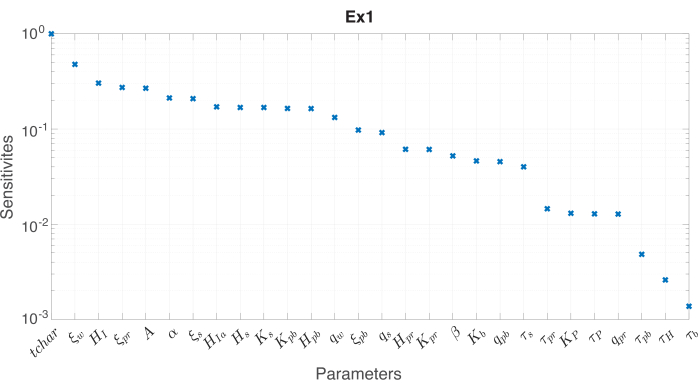
Figure 10: Sensitivity of model parameters to prediction of heart rate. The model and parameters are discussed in detail in the study by Randall et al.²⁰, and the estimated parameters are explained in Table 2. Please click here to view a larger version of this figure.

15. Optimization (Operation 10)

NOTE: This operation estimates a subset of identifiable parameters given the mathematical differential equations model and data availability (HR). The outcome is an HR model calibrated to data subsampled at 10 Hz. In addition to a set of estimated parameters, the optimized model predicts sympathetic and parasympathetic signals. If the simulation does not fit the data well, the predicted sympathetic and parasympathetic signals cannot be interpreted. Optimization is conducted using the Levenberg Marquardt method as described by Randall et al.²⁰.

1. The parameter estimation can take 5-10 min to complete. During computation, the MATLAB command window prints up to 30 lines of five numbers denoting (from left to right) the gradient norm, the least squares cost, the iteration number, and the Jacobian matrix condition number. When the optimization is complete, and continue to Operation 11 (Plot model predictions). The estimated parameter and a vector INDMAP are saved in the folder Optimized.

16. Plot model predictions (Operation 11)

NOTE: The results of model predictions with nominal (Step 13, Operation 8) and estimated (Step 15, Operation 10) parameter values are plotted at a resolution of 10 Hz corresponding to the subsampled data. If the HR prediction shown in the top right panel of MFigure 1 is reasonable, the code predicts sympathetic and parasympathetic signaling (Bottom right panel of MFigure 1).

1. On the menu, Select model predictions to view, click Nominal to plot the model predictions from Step 13 and Optimized to view the optimized model predictions from Step 15. MFigure 1 (Figure 11A nominal parameters, and Figure 11B optimized parameters) depicts BP (mmHg) in the top left corner, HR (bpm) in the top right corner data (blue), and the model (magenta), the thoracic pressure (Pth, mmHg) is at the bottom left corner. The prediction of parasympathetic (magenta) and sympathetic (dark purple) signals are in the bottom right corner. Click Save and exit, and continue to Operation 12 (Summary). This figure will be saved in the folder Figures/Model_fits under the name [patient name] + _[action].pn, where [action=nominal] or [action=optimal] depending on the chosen action.

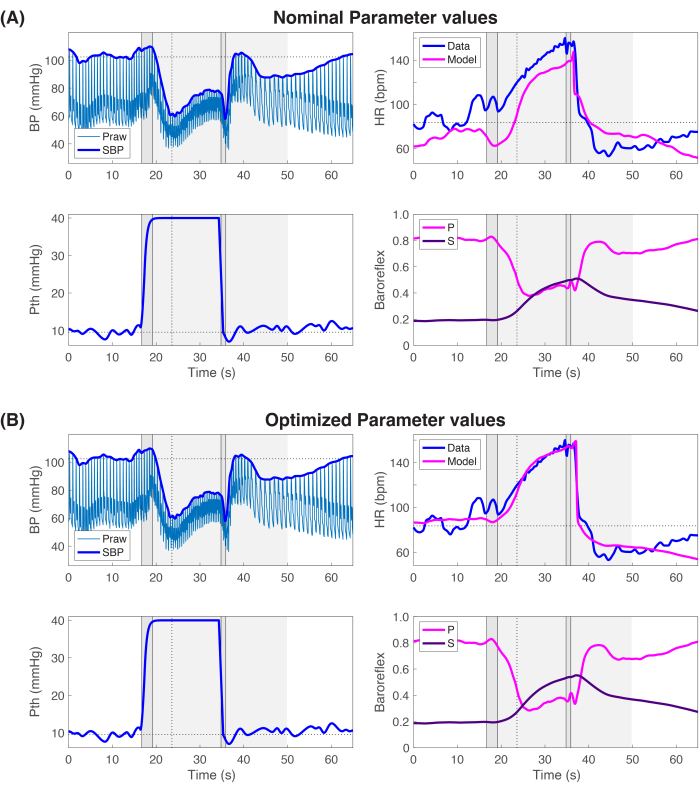
Figure 11: Model prediction. The model was predicted with (A) nominal and (B) optimized parameter values. The figure shows top left: blood pressure (SBP thick blue line and continuous BP light blue line, mmHg); top right: heart rate (HR, bpm), model prediction (pink line) and data (blue line); bottom left: thoracic pressure (Pth, mmHg) dark blue line; and bottom right: predictions of parasympathetic (pink) and sympathetic (purple) activity. Both are non-dimensional. Please click here to view a larger version of this figure.

17. Summary (Operation 12)

1. A summary of findings is stored as an Excel spreadsheet (.xlsx) and as a comma-separated file (.csv). The menu Save Data queries: Enter data summary file name (ex: FileName), enter the preferred name into the textbox. 
2. If the files exist, a menu queries the user: Add or overwrite the existing file. This operation also prints outputs to the MATLAB command line. Click OK to generate the file and Cancel to output only to the command line. The saved file (.xlxs and .cvs) contains patient information (Operation 1, Step 6), Clinical Markers and Regression Lines (Operation 7, Step 12), and Nominal (or Optimized) parameter values (Operation 11, Step 16). For each regression line, the R² value indicates the goodness of fit.
   NOTE: This operation (Step 17) can be completed without running the modeling, sensitivity, and optimization steps (Operations 8-11).

Results

The eight example datasets are selected to represent a diverse range of responses. Figure 3, Figure 4, Figure 5, Figure 6, Figure 7, Figure 8, Figure 9, Figure 10, and Figure 11 present the results from a representative healthy control subject for each ste...

Discussion

The ValsalvaAnalyzer software demonstrated in this study provides functionality to analyze clinical ECG and BP data recorded during the Valsalva maneuver. The software offers the ability to clean noisy signals, making it feasible to get consistent measures across a population. Using the corrected data, the software computes more than 35 markers that the user can interpret. The software aims to include all known quantities reported during the Valsalva maneuver reported in several studies^1,

Materials

List of materials used in this article

Name	Company	Catalog Number	Comments
LabChart	ADInstruments		Software that the data analyzed are exported from
MATLAB	Mathworks		Software used for the ValsalvaAnalyzer program

References

- Palamarchuk, I., Baker, J., Kimpinski, K. The utility of Valsalva maneuver in the diagnoses of orthostatic disorders. Am J Physiol. 310 (3), R243-R252 (2016).
- Pstras, L., Thomaseth, K., Waniewski, K., Balzani, I., Bellavere, F. The Valsalva manoeuvre: physiology and clinical examples. Acta Physiologica. 217 (2), 103-119 (2016).
- Singer, W., OpferGgehrking, T., McPhee, B., Hilz, M., Low, P. Influence of posture on the Valsalva manoeuvre. Clin Sci (London). 100 (4), 433-440 (2001).
- Groth, P., Tjernström, O. Pressure chamber tests for selection of aircrew. ORL J Otorhinolaryngol Relat Spec. 46 (5), 264-269 (1984).
- Gelfman, D. The Valsalva maneuver, set in stone. Am J Med. 134 (6), 823-824 (2021).
- Pstras, L., Thomaseth, K., Waniewski, J., Baizani, I., Bellavere, F. Mathematical modelling of cardiovascular response to the Valsalva manoeuvre. Math Med Biol. 34 (2), 261-292 (2017).
- Barbato, A. Chapter 78 - The History, Physical, and Laboratory Examinations. , Butterworths. (1990).
- Low, P., et al. Effect of age and gender on sudomotor and cardiovagal function and blood pressure response to tilt in normal subjects. Muscle Nerve. 20 (12), 1561-1568 (1997).
- Ewing, D., Martyn, C., Young, R., Clarkea, B. The value of cardiovascular autonomic function tests: 10 years experience in diabetes. Diabetes Care. 8 (5), 491-498 (1985).
- Nagar, A., Dhingra, N. Valsalva retinopathy. Postgrad Med J. 93 (1097), 174(2017).
- Sandroni, P., Novak, V., Opfer-Gehrking, T., Huck, C., Low, P. Mechanisms of blood pressure alterations in response to the Valsalva maneuver in postural tachycardia syndrome. Clin Auton Res. 10 (1), 1-5 (2000).
- El-Khayat, A. Valsalva haemorrhagic retinopathy in pregnancy after yoga. BMJ Case Rep. 2017, bcr2017221099(2017).
- Low, P. Testing the autonomic nervous system. Semin Neurol. 23 (4), 407-421 (2003).
- Won, H., Kim, P., Lee, J. Changes in echogenicity of hepatic hemangiomas during the Valsalva maneuver. J Clin Ultrasound. 45 (6), 328-331 (2017).
- Ricci, S., Moro, L., Minotti, G., Incalzi, R., De Maeseneer, M. Valsalva maneuver in phlebologic practice. Phlebology. 33 (2), 75-83 (2018).
- Felker, G., Cuculich, P., Gheorghiade, M. The Valsalva maneuver: a bedside "biomarker" for heart failure. Am J Med. 119 (2), 117-122 (2006).
- Kim, J., et al. Utility of corrected QT interval in orthostatic intolerance. PLoS One. 9 (9), e106417(2014).
- Kim, H., Yi, H., Hong, J., Lee, H. Detailed relationship between the pattern of blood pressure change during the Valsalva maneuver and the degree of orthostatic hypotension during the head-up tilt test in patients with orthostatic intolerance: a retrospective case-control study. Medicine (Baltimore). 95 (19), e3608(2016).
- Bingger, W., Mitchell, R., Harron, D., McKaigue, J., McAloney, R. Real time analysis of Valsalva maneuver. Comput BIol Med. 19 (5), 319-329 (1989).
- Randall, E., Billeschou, A., Brinth, L., Mehlsen, J., Olufsen, M. A model-based analysis of autonomic nervous function in response to the Valsalva maneuver. J Appl Physiol. 127 (5), 1386-1402 (2019).
- Motamedi, M., Akbarzadeh, M., Safari, S., Shahhoseini, M. Valsalva maneuver using a Handmade Device in Supraventricular Tachycardia Reversion; a quasi experimental study. Emerg (Tehran). 5 (1), e81(2017).
- Abdulhamid, A., et al. Modified Valsalva versus standard Valsalva for cardioversion of supraventricular tachycardia: systematic review and meta-analysis. Int J Arrhythmia. 22, 2(2021).
- VitalScan. The future of health care autonomic nervous system testing. , (2023).
- Heart rate variability (HRV) software. , Kubios. (2023).
- Robertson, D., Biaggioni, I., Burnstock, G., Low, P. A., Paton, J. Primer on the autonomic nervous system. , Elsevier. (2012).
- Hristovska, A., et al. Orthostatic intolerance after acute mild hypovolemia: incidence, pathophysiologic hemodynamics, and heart-rate variability analysis-a prospective observational cohort study. Can J Anaesth. 70 (10), 1587-1599 (2023).
- Hristovska, A., Uldall-Hansen, B., Mehlsen, J., Kehlet, H., Foss, N. Orthostatic intolerance after intravenous administration of morphine: incidence, haemodynamics and heart rate variability analysis. Anesthesia. 78 (4), 526-528 (2022).
- Geddes, J., Ottesen, J., Mehlsen, J., Olufsen, M. Postural orthostatic tachycardia syndrome explained using a baroreflex response model. JR Soc Interface. 19 (193), 20220220(2022).
- Overweight and obesity. , Centers for Disease Control and Prevention. https://www.cdc.gov/obesity/index.html (2022).
- Denq, J., O'Brian, P., Low, P. Normative data on phases of the Valsalva maneuver. J Clini Neurophysiol. 15 (6), 535-540 (1998).
- Sandroni, P., Benarroch, E., Low, P. Pharmacological dissection of components of the Valsalva maneuver in adrenergic failure. J Appl Physiol. 71 (4), 1563-1567 (1985).
- Huang, C., Sandroni, P., Sletten, D., Weigand, S., Low, P. Effect of age on adrenergic and vagal baroreflex sensitivity in normal subjects. Muscle Nerve. 36 (5), 637-642 (2007).
- Novak, P. Assessment of sympathetic index from the Valsalva maneuver. Neurology. 76 (23), 2010-2016 (2011).
- Wada, N., et al. Determination of vagal baroreflex sensitivity in normal subjects. Muscle Nerve. 50 (4), 535-540 (2014).
- Wada, N., et al. Comparison of baroreflex sensitivity with a fall and rise in blood pressure induced by the Valsalva manoeuvre. Clin Sci (London). 127 (5), 307-313 (2014).
- Schrezenmaier, C., et al. Adrenergic and vagal baroreflex sensitivity in autonomic failure. Arch Neurol. 64 (3), 381-386 (2007).
- Trefethen, L. Spectral methods in Matlab. , SIAM. (2000).
- Moštak, I., Višnjić, N., Junaković, A., Skorić, M. Comparison of baroreflex sensitivity indices with standard tests of autonomic system function. J Neurol Sci. 426, 117473(2021).
- García, J., López, A., Stefan, M., Milner, D. Influence of repetitions on the Valsalva maneuver. Neurophysiol Prac. 5, 104-111 (2020).
- Vogel, E., Sandroni, P., Low, P. Blood pressure recovery from Valsalva maneuver in patients with autonomic failure. Neurology. 65 (10), 1533-1537 (2005).
- Kobayashi, H. Normalization of respiratory sinus arrhythmia by factoring in tidal volume. Appl Human Sci. 17 (5), 207-213 (1998).
Access restricted. Please log in or start a trial to view this content.
Reprints and Permissions