Quantification of Adeno-Associated Viral Genomes in Purified Vector Samples by Digital Droplet Polymerase Chain Reaction

Summary

Precise quantification of adeno-associated virus (AAV) vector genome copies is critical, but a standardized protocol has yet to be established. This protocol describes a validated method for preparing purified AAV samples and conducting digital droplet polymerase chain reaction (dd_PCR) to reliably quantify the viral genome titer.

Abstract

Adeno-associated virus (AAV) is a non-pathogenic virus used as a delivery vehicle to transfer therapeutic genes into patients. Accurate quantification of AAV genome copy number in vector preparations is essential for bioprocess optimization and dosage calculation in both preclinical and clinical studies of AAV-based gene therapy products. Currently, a consensus protocol for AAV viral genome titration is lacking. Here, we present a digital droplet PCR (dd_PCR) protocol for the quantification of viral genomes in purified vector samples. Samples are treated with DNase I to eliminate unpackaged contaminant DNA. DNase-treated samples are then mixed with an appropriate primer-probe set (designed according to the target AAV genome) and PCR reagents, and then loaded into a droplet generator. The prepared droplets are transferred into a PCR plate, where PCR amplification is performed and analyzed. The viral genome titer is calculated based on the concentration (copies/µL), accounting for sample dilutions. A successful measurement shows a clear separation of the positive and negative droplet clouds, has at least 10,000 accepted droplets, shows a value between 10 copies/µL and 10,000 copies/µL, and has a coefficient of variation (CV) between repeats lower than 20%. Reliable viral genome titration will aid in the development of safe and effective AAV-based gene therapy products.

Introduction

Gene therapy is a therapeutic modality commonly used to treat genetic disorders. The design of any given gene therapy is specific to the associated pathology of the target indication, but all gene therapies involve the intracellular delivery of genetic material to target cells in order to elicit a therapeutic effect¹. Gene therapy can be further classified into several categories, including gene replacement for loss-of-function mutations, gene silencing for gain-of-function abnormalities, and gene editing techniques. Irrespective of the specific strategy employed, the therapeutic nucleic acid material (referred to as a transgene) must be packaged within a vector in order to achieve targeted intracellular delivery².

Although a variety of viral and non-viral vector systems are available for gene therapy development, adeno-associated viruses (AAVs) are frequently chosen due to the broad viral tropism and low immunogenicity associated with this group of viruses^1,2. To date, seven gene therapies utilizing AAV for therapeutic gene delivery have achieved approval from either the European Medicines Agency (EMA) or the Food and Drug Administration (FDA) targeting diseases ranging from hemophilia (e.g., Roctavian) to spinal muscular atrophy (e.g., Zolgensma)³.

Production of AAV-based gene therapies stems from an understanding of the wild-type AAV itself. AAV is a small DNA virus within the Parvoviridae family comprising 13 main serotypes (AAV1-13)³. The AAV genome comprises a ~4.7 kb, single-stranded DNA molecule containing two main open reading frames (ORFs) that encode the essential viral genes necessary for genome replication, capsid assembly, and packaging (rep, cap). The viral genome is flanked at both the 5' and 3' ends by palindromic nucleotide sequences, referred to as inverted terminal repeats (ITRs). These ITRs form hairpin-like structures that play crucial roles in genome replication and packaging of de novo viral genomes into newly synthesized viral capsids. AAV is a helper-dependent virus and, therefore, requires the expression of ancillary genes from other viruses, such as herpes simplex virus (HSV) or adenovirus (AdV) in order to become replication-competent¹.

In order to produce AAVs, a suitable cell-based expression system is employed to facilitate the expression of the viral capsid proteins and subsequent assembly into de novo viral particles, followed by encapsidation of an ITR-flanked selected transgene (also referred to as a vector genome). This process commonly utilizes a triple plasmid system, comprising (1) a plasmid harboring helper genes derived from a helper virus, (2) a plasmid encoding the essential viral elements (rep/cap), and (3) a plasmid carrying the therapeutic expression cassette (commonly referred to as a transfer plasmid)⁴. The unique presence of inverted terminal repeat (ITR) packaging signals flanking the therapeutic expression cassette in the transfer plasmid ensures specific packaging of the transgene, while mostly excluding the viral genes present on the other plasmids. Co-transfection of this three-plasmid system into a cell-based expression platform (typically HEK293T cells) results in the production of transduction-competent, replication-deficient viral particles suitable for use in gene therapy applications^3,4.

There are a number of critical quality attributes (CQAs) associated with the production of AAV-based gene therapies that must be assessed in order to ensure the potency, purity, and safety of the intended medicinal product⁴. These CQAs include virus titer, capsid content, and aggregation. Virus titer itself is a combination of the number of viral particles (capsid titer) and the number of vector genomes (vector genome titer) present in any given preparation. Ideally, the ratio between these two titers should be 1:1 since each viral particle should contain one vector genome, but inefficiencies in vector genome packaging during biosynthesis result in the co-production of empty or partially filled capsids (those containing partial vector genome sequences and/or non-vector genome sequences)⁵. The presence of such impurities can potentially evoke unwarranted immune responses and compete for vector-binding sites, thereby increasing the risk of immunotoxicity and reducing the rate of transduction of full capsids⁶. Accurate quantification of AAV genomes is therefore essential for establishing virus titer and capsid content. This impacts both basic research as well as the gene therapy industry, which requires accurate dosage in order to maintain both the safety and efficacy of medicinal products.

Digital Droplet polymerase chain reaction (dd_PCR) has become closely associated with the quantification of virus titer since it can be utilized to determine the number of vector genomes present in any given preparation⁷. Digital PCR itself was first introduced in the 1990s^8,9 and dd_PCR is an enhancement to this technology that allows for high-throughput sample processing^10,11. In dd_PCR, a 20 µL real-time PCR reaction is partitioned into approximately 20,000 oil-encased droplets, giving up to 96 such reactions when accommodated on a standard 96-well plate. Compared with conventional quantitative PCR (qPCR), dd_PCR offers several advantages, including enhanced sensitivity, increased precision, and more direct and absolute quantification of target sequences without the need for standard curves. Moreover, the high level of partitioning in dd_PCR reduces the impact of PCR inhibitors and minimizes the potential for bias from preferential amplification of certain templates, making it an attractive option for analytical measurement of vector genome titration.

Protocol

The protocol described here is designed to quantify the viral genome titer of a purified, in-house produced AAV9 vector with green fluorescent protein (GFP) as the transgene¹² with a high level of precision (Table 1). However, this protocol is applicable to any AAV serotype and any vector genome design, provided that the primer/probe sets are designed to target the specific vector genome of interest. Details of the reagents, primers, probes, and equipment used in this study are listed in the Table of Materials.

1. Preparation of stock solutions

NOTE: Prepare all stock solutions required for sample dilution at a PCR workstation to avoid contamination from foreign DNA.

1. Prepare 10x PCR assay buffer, which consists of 500 mM of KCl, 100 mM of Tris-HCl, 15 mM of MgCl_2, and 0.01 % (w/v) BSA. Measure the pH of the solution and adjust it to 8.3.
   NOTE: This solution can be kept at room temperature for up to 1 month.
2. Prepare the AAV dilution buffer, which consists of 1x PCR assay buffer, 0.2 ng/µL salmon sperm sheared (sss) DNA, and 0.1 % pluronic F-68. Make this solution freshly with each assay and keep it at 4 °C.
   NOTE: If pluronic F-68 is not available, an alternative such as Poloxamer 188 non-ionic surfactant could be used.

2. Preparation of samples - DNase I treatment and serial dilution

NOTE: In order to remove DNA contaminants that could lower the accuracy of the vector genome titration, free DNA present within the AAV sample (including remaining plasmid DNA or non-encapsidated viral genomes) can be removed prior to PCR amplification using DNase. This is possible since the vector genomes are encapsidated within the AAV capsids and are therefore not accessible until the denaturing step of the PCR reaction itself (see step 5). Furthermore, since the vector genome number in any given sample is unknown, it is necessary to perform a serial dilution of the samples to ensure measurements remain within the upper and lower detectable limits. Perform all sample manipulations at a PCR workstation. Keep all samples on ice unless specified otherwise.

1. Mix the AAV sample selected for analysis by briefly vortexing and then centrifuging to ensure all liquid remains at the bottom of the tube containing the sample.
2. For DNase treatment, add 45 µL of a solution containing 1x DNase I buffer, 0.1% pluronic F-68, and 0.04 U/µL DNase I in DNase-free water into a 0.2 mL PCR 8-tube strip tube.
3. Transfer 5 µL of sample into the tube containing the DNAse solution. Vortex the samples and briefly centrifuge to ensure all liquid remains at the bottom.
4. In a thermocycler, incubate the samples for 1 h at 37 °C, then cool down to 4 °C. Place on ice as soon as possible after 4 °C is reached.
5. Using a fresh 0.2 mL PCR 8-tube strip, make appropriate dilutions of the DNase-treated sample in AAV dilution buffer. Recommended sample dilutions depend on the expected vg titer (Table 2), but aim for at least 2 different dilutions per sample and run each dilution in duplicate. Ensure to rigorously (2,000-3,000 rpm) vortex the samples for 5 s before taking out any volume.
6. After serial dilution, vortex the samples and centrifuge to ensure all liquid remains at the bottom of the tubes.
7. Include a positive control of which vg titer is known, and a negative control (AAV dilution buffer only) which is also called the no template control (NTC).
   NOTE: The positive control can be an in-house produced AAV or a commercial AAV reference material, which includes the target sequence of the primers/probe.

3. Preparation of dd_PCR master mix

NOTE: Select an appropriate target sequence within the vector genome and design a forward primer, reverse primer, and hydrolysis probes labeled with FAM or HEX reporter fluorophores following published guidelines¹³. Primers that target the transgene are preferred over primers that target the ITRs since the transgene is specific to the vector genome design, and the secondary structure associated with the hairpin formation of the ITRs can hamper efficient primer binding. Moreover, ITR primers might overestimate AAV titers if partially filled capsids that contain truncated vector genome fragments are present and still house either of the ITR sequences¹⁴. Prepare the dd_PCR master mix in a dedicated, separate workstation (pre-PCR room). This room should be separate from the one where the samples are prepared to avoid cross-contamination.

1. Allow the primer, probe, and dd_PCR supermix reagents to reach room temperature (20-25 °C). Afterward, vortex all reagents and briefly centrifuge the tubes to collect all liquid at the bottom of the tube.
2. Prepare a volume of dd_PCR master mix in a separate microcentrifuge tube according to the required number of reactions by combining the forward and reverse primers, probe, dd_PCR supermix, and DNase-free water according to the volumes and concentrations described in Table 3.
   1. Vortex the master mix and then briefly centrifuge the tube to ensure all liquid remains at the bottom of the tube.
      NOTE: Always prepare extra dd_PCR master mix volume than required (n + 1) in order to account for pipetting volume loss.
3. Transfer 19.8 µL of the master mix into each tube on a fresh 0.2 mL PCR 8-tube strip.

4. Droplet generation

NOTE: Samples and dd_PCR master mix are mixed separately prior to loading into a droplet-generating cartridge. Perform all manipulations at a PCR workstation, preferably a different one from where the samples were prepared, to avoid amplicon contamination. Alternatively, clean the PCR workstation thoroughly after preparing the samples.

1. Transfer 2.2 µL of the diluted sample into the 19.8 µL volume of dd_PCR master mix in each tube of the PCR 8-tube strip and mix well. Vortex and briefly centrifuge to ensure all liquid remains at the bottom.
2. Transfer 20 µL of this solution into the wells contained in the middle "sample" row of a droplet-generating cartridge. Avoid bubbles in the droplet-generating cartridge; this can cause the instrument to give errors, and droplets will fail to be generated.
   NOTE: Since the cartridges are in 8-well format, as are the PCR tube strips, it is recommended that an 8-channel pipette be used.
3. Transfer 60 µL of the droplet-generation oil to the wells contained on the lower "oil" row of the droplet-generating cartridge.
   NOTE: Never leave a well of the droplet-generating cartridge empty; fill the empty sample well with dd_PCR buffer control for probes (with the corresponding volume described above).
4. Place a rubber gasket over the droplet-generating cartridge and place it in the droplet generator.
5. After the droplets are generated, use an 8-channel pipette to slowly transfer 42.5 µL solution from the dd_PCR chip to a multi-well PCR plate.
   NOTE: Pipette slowly and at a 45-degree angle to avoid droplet shearing in the liquid while pipetting. Visually inspect the plate so that all wells are filled with the same amount of liquid and droplets are visible as an opaque layer in the well.
6. Seal the plate with an aluminum foil cover in a heat-sealing machine for 5 s at 180 °C.
   NOTE: Visually inspect that all wells are sealed. If not, repeat another 5 s at 180 °C. The sealed plate can be kept for up to 4 h at 4 °C before dd_PCR amplification in a thermal cycler.

5. dd_PCR amplification

NOTE: The thermal cycler should be placed in a separate room from the pre-PCR room to spatially separate pre-PCR activities from PCR amplification and avoid false-positive results due to amplicon contamination.

1. Place the plate in a thermal cycler (with a 96-deep well reaction module) for PCR amplification and close it securely.
2. Configure the thermocycler to run at the conditions described in Table 4 and at a reaction volume of 40 µL. Include a pre-heating step in the program settings and ensure the lid is heated to 99 °C.
3. When the PCR program is over, keep the plate at 4 °C for at least 15 min to ensure that the plate is fully cooled down.
   NOTE: The plate can be kept for 48-72 h at 4 °C before the droplets have to be read.

6. Droplet reading

1. Load the plate into a droplet reader, input the following information in the system software, and continue the reading.
   NOTE: Experiment type = Direct quantification; Supermix = dd_PCR supermix for probes (no dUTP); Assay type = single target per channel; Target info, signal channel 1 = FAM channel or HEX channel according to the used probe.
2. Annotate the samples so that the position of each sample can be determined and identified effectively from the data file.

7. Data analysis

1. Carry out the data analysis using the compatible software provided by the droplet reader manufacturer.
2. Carry out a system suitability test to evaluate the overall performance (and, therefore, reliability) of the assay.
   1. Check the event count (number of droplets) measured for each well on the PCR plate. Ideally, the event count is between 15,000 and 20,000. If the event count is <10,000, then this value must be excluded from the analysis.
   2. Evaluate the 1D or 2D amplitude plot and check for the presence of droplet rain.
   3. Go to the data table tab and export the data to an Excel file.
3. Calculate vg titer following the steps below:
   1. The working range of dd_PCR is 10-10 000 copies/µL. Exclude any value that is <10 copies/µL from the analysis. The recommended range for the dd_PCR equipment used herein is 25-5000 copies/µL.
      NOTE: The data analysis software will provide a vector genome number in accordance with the PCR reaction volume (40 µL), but this does not take into consideration the dilution factors applied during sample preparation.
   2. Calculate the sample vg titer per volume (typically expressed as vg/mL) by factoring in the various dilution factors throughout the sample preparation using the following relation:
      NOTE: Concentration (value obtained from data analysis) x 10 (DNase I pre-treatment dilution) x 10 (PCR master mix dilution) x 1000 (µL to mL) selected sample dilution (in AAV dilution buffer - e.g., Table 2).
   3. Calculate the coefficient of variation (%CV) between the replicates and between the different dilutions of the same sample.
      NOTE: %CV is calculated by dividing the standard deviation by the mean. If the %CV between the different dilutions is >20 %, the value should not be considered accurate.
   4. Check the values of the negative and positive control. The negative control should be less than 5 copies/µL.

Results

Results can be visualized using appropriate software. For each well, the 1D amplitude plot displays all droplets relative to their amplitude. A clear separation between positive and negative droplets is expected. If more than 10% of the total droplets are found between the positive and negative droplet clouds (a phenomenon referred to as droplet rain), it is necessary to re-measure the sample (see Figure 1). Additional information on droplet rain is available in the discussion.

A data table can be created to summarize all recorded information, including the sample name, number of accepted droplets (event counts), and concentration (copies/µL). Ideally, the event count should fall between 15,000 and 20,000 accepted droplets. If the event count for a well is below 10,000, the data point should be excluded from the analysis. An example of the output data is provided in Table 5.

The vg titer can be calculated based on the concentration (copies/µL), with consideration of sample dilutions. The working range of dd_PCR is 10-10,000 copies/µL. Values below 10 copies/µL should be excluded from the analysis. The vg titer for samples, as well as the positive and negative controls, should be calculated. The measured value of the positive control should have a coefficient of variation (%CV) lower than 20% relative to the theoretical value. The negative control should be less than 5 copies/µL. Additionally, the %CV between repeats and different dilutions for each sample should be calculated. If the %CV between different dilutions exceeds 20%, the value may be considered inaccurate, and the sample may need to be re-measured.

A successful measurement is characterized by a clear separation of the positive and negative droplet clouds, at least 10,000 accepted droplets, a value between 10 copies/µL and 10,000 copies/µL, and a %CV between repeats lower than 20%.

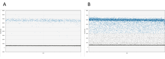
Figure 1: Visualization of dd_PCR droplets. (A) The 1D amplitude plot demonstrates a clear separation of positive and negative droplets, indicating successful droplet partitioning. (B) The plot shows a poor separation of positive and negative droplets, known as droplet rain, which suggests suboptimal partitioning or potential issues with the assay. Please click here to view a larger version of this figure.

Figure 2: Workflow for quantifying viral genomes using digital droplet PCR. (1) Buffers, reagents, and solutions are prepared according to the manufacturer's instructions or step 1 of the protocol (Preparation of stock solutions). (2) 45 µL of the DNase I solution is aliquoted into each tube of an 8-tube PCR strip. After vortexing and briefly centrifuging the samples, 5 µL of the sample is added to one of the tubes. The DNase I and sample-containing eight-tube PCR strip are incubated in a thermocycler for 1 h at 37 °C, followed by serial dilutions of the samples. (3) The PCR mastermix is prepared as described, and 19.8 µL is aliquoted into each tube of an 8-tube PCR strip. Sample serial dilutions from step 2 are added to the mastermix. 20 µL of the mastermix plus
sample solution is loaded into the middle row of the cartridge, and 60 µL of droplet-generation oil is transferred to the lower wells of a droplet-generating cartridge. The cartridge is then placed into the droplet generator and run according to specified conditions. After droplet generation, 42.5 µL from the top row of the cartridge is transferred to a multi-well PCR plate. (4) The PCR plate is loaded into a PCR thermocycler and run according to the provided conditions. The plate is analyzed using a dd_PCR reader. Please click here to view a larger version of this figure.

Table 1: Precision data. This table presents precision data from four sets of quality control (QC) samples, each with five concentrations (QC1-QC5). Each QC was measured five times. The coefficient of variation (%CV) between different runs, representing repeatability (A), and between different sets of samples, representing intermediate precision (B), is shown. Please click here to download this Table.

Table 2: Sample dilutions. The table shows the recommended sample dilutions based on the expected viral genome titer (vg/mL). A total of three dilutions are recommended to ensure at least two values fall within the working range of the assay. Please click here to download this Table.

Table 3: dd_PCR master mix composition. This table outlines the composition of the dd_PCR master mix, which includes a forward and reverse primer (909 nM), probe (227 nM), and dd_PCR supermix for probes (without dUTP, 1x). Please click here to download this Table.

Table 4: Thermocycling conditions. The table details the recommended PCR program, which includes: (1) a 10 min incubation at 95 °C for capsid disruption and enzyme activation, (2) 40 cycles of 30 s at 94 °C for DNA denaturation, and 1 min at 60 °C for annealing and extension, (3) a 10 min incubation at 98 °C for enzyme deactivation, and (4) holding at 4 °C. The annealing temperature may require optimization based on the primer/probe set used. Please click here to download this Table.

Table 5: Example of output data from an actual AAV run. The table provides an example of output data from an actual AAV run, where one sample was measured in two different dilutions, each in duplicate. The viral genome (vg) titer (in vg/mL) is calculated using the following formula: 10 (DNase I pre-treatment) x 10 (dilution in the master mix) x 1,000 (µL to mL) x dilution in AAV dilution buffer. STDEV represents standard deviation, and CV indicates the coefficient of variation. Please click here to download this Table.

Discussion

Accurate quantification of AAV vector genome copies in vector preparations is essential for the development of AAV-based gene therapy products. Several methods exist for determining the vg titer, with quantitative PCR (qPCR) and dd_PCR being the two most widely used and accepted techniques. dd_PCR is often preferred over qPCR due to its independence from amplification efficiency, higher precision, and greater robustness¹⁵. Numerous protocols for vector genome titration by dd_PCR are available in the literature, each with its own sample preparation methods^15,16,17. However, there is a lack of a qualified consensus protocol. This article presents a validated fit-for-purpose dd_PCR protocol for the quantification of AAV vector genomes in purified vector samples (Figure 2).

Close attention to sample handling is critical when performing this protocol. Cross-contamination can pose a significant challenge in accurately assessing vg titers; therefore, samples are best processed under a PCR workstation to avoid contamination with foreign DNA. Additionally, proper execution of DNase incubation is crucial to eliminate unpackaged contaminant DNA without disrupting the capsid and potentially digesting the packaged vector genome. Many protocols include heat inactivation and proteinase K treatment^16,17,18. However, during in-house method development, it was found that excessive heating was detrimental to vg titration, and proteinase K treatment was unnecessary (data not shown).

As dd_PCR becomes increasingly popular for quantifying viral genomes, manufacturers have published detailed application guides with guidelines on designing and optimizing dd_PCR assays¹⁹. Troubleshooting information is also available. In practice, when an assay is correctly designed, the most frequent issues include droplet rain and low droplet count. Droplet rain is often caused by poor accessibility of the primer/probes to the amplicon, but several strategies can address this issue. For instance, a temperature gradient experiment can help establish the optimal annealing temperature. Additionally, diluting samples to lower the DNA amount (recommended to be less than 66 ng) or performing a restriction digest with specific enzymes that cut outside the amplicon region can improve template accessibility. A recommendation of 10 U of restriction enzyme per µg of DNA is typically effective. The issue of low droplet count (fewer than 10,000) is frequently due to poor pipetting of the sample and oil in the cartridges. Slow pipetting with appropriate tips is recommended to avoid shearing of the droplets. While the dd_PCR assay is robust, one limitation is the extended time to result. The process from sample treatment to droplet reading takes several hours, which can be a drawback when results are needed quickly.

Accurate quantification of AAV genome copies in vector preparations is necessary throughout all stages of the AAV gene therapy life cycle. Specifically, it is important for optimizing production and purification processes, conducting preclinical studies, and determining clinical dosages for AAV-based gene therapy products. The dd_PCR protocol presented here is broadly applicable and can be used on purified AAV products with different serotypes and transgenes.

Materials

List of materials used in this article

Name	Company	Catalog Number	Comments
8-channel pipette 10 µL	Eppendorf	3,12,50,00,010
8-channel pipette 200 µL	Eppendorf	3,12,50,00,036
8-channel pipette 300 µL	Eppendorf	3,12,50,00,052
8-well PCR strip	Sarstedt	72.991.002
Bovine Serum Albumin (BSA)	Sigma-Aldrich	A9418
C1000 Touch Thermal Cycler with 96–Deep Well Reaction Module	Bio-Rad	1851197
ddPCR Buffer Control for Probes 9 mL (2 x 4.5 mL)	Bio-Rad	1863052
ddPCR Supermix for Probes (No dUTP) (2 x 1 mL)	Bio-Rad	1863023
ddPCR 96-Well Plates (pkg of 25)	Bio-Rad	12001925
ddPCR Droplet Reader Oil (2 x 1L)	Bio-Rad	1863004
DG8 Cartridge Holder	Bio-Rad	1863051
DG8 Cartridges for QX200/QX100 (pkg of 24)	Bio-Rad	1864008
DG8 Gaskets for QX200/QX100 (pkg of 24)	Bio-Rad	1863009
DNase I (10U/µL) + buffer	Roche	4716728001
Droplet Generation Oil for Probes (10 x 7 mL)	Bio-Rad	1863005
Eppendorf ep Dualfilter T.I.P.S. Filter Tip, 0.1-10 μL, 34 mm, Rack, PCR Clean, STERILE	Eppendorf	30078500
Eppendorf ep Dualfilter T.I.P.S. Filter Tip, 20-300 μL, 55 mm, Rack, PCR Clean, STERILE	Eppendorf	30078560
Eppendorf ep Dualfilter T.I.P.S. Filter Tip, 2-100 μL, 53 mm, Rack, PCR Clean, STERILE	Eppendorf	30078543
Forward lyophilized primers and respective master stocks at 100 mM	IDT		GFP as target sequence. Forward primer: 5'-GAACGGCATCAAGGTGAACT-3'
Lyopohilized probe and master stock at 100 µM	IDT		GFP as target sequence. PrimeTime Eco Probe: /56-FAM/CAAGATCCG/ZEN/CCACAACATCGAGGA/3IABkFQ/
Magnesium Chloride (MgCl2)	Chemlab Analytical	CL00.1381
Nuclease free water	IDT	11-04-02-01
PCR Plate Heat Seal, foil, pierceable (pkg of 100)	Bio-Rad	1814040
Pluronic F-68 non-ionic surfactant (100x)	Thermo Fisher Scientific	24040032
Potassium Chloride (KCl)	Honeywell research chemicals	31248
QX manager software	Bio-Rad		Software to analyse ddPCR data
QX200 Droplet Generator	Bio-Rad	1864002
QX200 Droplet Reader	Bio-Rad	1864003
Reagent reservoir	VWR	613-1181
Reverse lyophilized primers and respective master stocks at 100 mM	IDT		GFP as target sequence. Reverse primer: 5'-TGCTCAGGTAGTGGTTGTCG-3'
SafeSeal reaction tube, 1.5 mL	Sarstedt	72.706.200
Salmon Sperm DNA, sheared (10 mg/mL)	Thermo Fisher Scientific	AM9680
TE buffer	IDT		Accompanied by primers when ordering
Tris hydrochloride (Tris-HCl)	Roche	10812846001

References

- Balakrishnan, B., Jayandharan, G. R. Basic biology of adeno-associated virus (AAV) vectors used in gene therapy. Curr Gene Ther. 14 (2), 86-100 (2014).
- Srivastava, A. In vivo tissue-tropism of adeno-associated viral vectors. Curr Opin Virol. 21, 75-80 (2016).
- Pupo, A., et al. AAV vectors: The Rubik's cube of human gene therapy. Mol Ther. 30 (12), 3515-3541 (2022).
- Gimpel, A. L., et al. Analytical methods for process and product characterization of recombinant adeno-associated virus-based gene therapies. Mol Ther Methods Clin Dev. 20, 740-754 (2021).
- Brimble, M. A., et al. Preventing packaging of translatable P5-associated DNA contaminants in recombinant AAV vector preps. Mol Ther Methods Clin Dev. 24, 280-291 (2022).
- Wright, J. F. Product-related impurities in clinical-grade recombinant AAV vectors: Characterization and risk assessment. Biomedicines. 2 (1), 80-97 (2014).
- Dobnik, D., et al. Accurate quantification and characterization of adeno-associated viral vectors. Front Microbiol. 10, (2019).
- Sidransky, D., et al. Identification of ras oncogene mutations in the stool of patients with curable colorectal tumors. Science. 256 (5053), 102-105 (1992).
- Vogelstein, B., Kinzler, K. W. Digital PCR. Proc Natl Acad Sci USA. 96 (16), 9236-9241 (1999).
- Hindson, B. J., et al. High-throughput droplet digital PCR system for absolute quantitation of DNA copy number. Anal Chem. 83 (22), 8604-8610 (2011).
- Pinheiro, L. B., et al. Evaluation of a droplet digital polymerase chain reaction format for DNA copy number quantification. Anal Chem. 84 (2), 1003-1011 (2012).
- Sanmiguel, J., Gao, G., Vandenberghe, L. H. Quantitative and digital droplet-based AAV genome titration. Methods Mol Biol. 1950, 51-83 (2019).
- Bio-Rad Laboratories Inc. Planning droplet digital PCR experiments. , https://www.bio-rad.com/en-in/life-science/learning-center/introduction-to-digital-pcr/planning-ddpcr-experiments (2024).
- Dorange, F., Le Bec, C. Analytical approaches to characterize AAV vector production & purification: Advances and challenges. Cell Gene Ther Insights. 4 (2), 119-129 (2018).
- Lock, M., et al. Absolute determination of single-stranded and self-complementary adeno-associated viral vector genome titers by droplet digital PCR. Hum Gene Ther Methods. 25 (2), 115-125 (2014).
- Prantner, A., Maar, D. Genome concentration, characterization, and integrity analysis of recombinant adeno-associated viral vectors using droplet digital PCR. PLoS One. 18 (1), e0280242(2023).
- Dobnik, D., et al. Accurate quantification and characterization of adeno-associated viral vectors. Front Microbiol. 10, 1570(2019).
- Suoranta, T., Laham-Karam, N., Yla-Herttuala, S. Optimized protocol for accurate titration of adeno-associated virus vectors. Hum Gene Ther. 32 (19-20), 1270-1279 (2021).
- Bio-Rad. Droplet digital PCR applications guide. Bulletin 6407. , https://www.bio-rad.com/webroot/web/pdf/lsr/literature/Bulletin_6407.pdf (2024).
Reprints and Permissions