Intravital Longitudinal Imaging of Vascular Dynamics in the Calvarial Bone Marrow

Summary

Intravital microscopy allows the study of dynamic biological processes such as tissue regeneration and tumor development. The calvarial bone marrow, a highly dynamic tissue, offers insights into hematopoiesis and vascular function. Using a biocompatible 3D-printed head fixation implant allows for repetitive longitudinal imaging, enhancing our understanding of tissue dynamics and the tumor microenvironment.

Abstract

Intravital longitudinal fluorescence microscopy imaging has emerged as a crucial technique for studying dynamic biological processes, notably in the context of tissue regeneration, tumor development, and therapeutic responses. Particularly, the calvarial bone marrow is a highly dynamic tissue, where the hematopoietic fate is interconnected with the surrounding microenvironment, with specialized vessels responding to normal and pathologic hematopoiesis. Traditional imaging of fixed tissues offers static information, often limiting a comprehensive understanding of these processes.

The integration of transgenic animals expressing cell-specific markers, live cell tracers, advancements in imaging equipment, and the use of specialized chambers has elevated intravital microscopy to a pivotal tool for gaining insights into dynamic biological phenomena. One application of intravital imaging is the investigation of tumor vessel behavior and therapeutic effects. A newly designed 3D-printed titanium head fixation implant can be stably connected to the mouse skull and is suitable for longitudinal imaging during multiple sessions.

The proposed protocol allows for the spatial and temporal examination of vascular dynamics in the calvarial bone marrow, including visualization and quantification of vascular heterogeneity, interaction with stromal and hematopoietic cells, and measurement of vascular functional parameters. Additionally, the technique enables the visualization of established vascular beds and the monitoring of therapeutic effects, stem cell mobilization, and the localization of chemotherapeutic compounds over time using two-photon microscopy. Overall, this intravital longitudinal imaging protocol provides a comprehensive platform for investigating both tumor vessel behavior and hematopoietic cell dynamics, offering valuable insights into the intricate processes governing these biological phenomena.

Introduction

Intravital microscopy imaging of the calvarial bone marrow (BM) serves as a powerful and indispensable technique for investigating the dynamic processes of hematopoiesis, tissue microenvironment regulation, and vascular dynamics within the BM niche. The primary purpose of this methodological approach is to enable real-time visualization and analysis of cellular behaviors, interactions, and spatial organization within the BM microenvironment in vivo. By directly observing the BM calvaria using advanced imaging techniques coupled with fluorescent labeling, researchers can elucidate the complex interplay between hematopoietic stem cells (HSCs), stromal cells, and the surrounding vasculature, thereby providing crucial insights into the regulation of hematopoiesis and immune responses.

The development and utilization of intravital microscopy imaging stem from the limitations of traditional histological and ex vivo imaging methods, which often fail to capture the dynamic nature of cellular behaviors and interactions within a tissue. Unlike static imaging techniques, intravital microscopy enables researchers to observe cellular dynamics in real time, allowing for the study of longitudinal processes such as cell migration, proliferation, and differentiation within their native niche, without sacrificing experimental animals. Furthermore, intravital microscopy provides the unique advantage of studying functional behaviors in vivo, such as vascular functionality (e.g., perfusion, permeability, hypoxia), thereby preserving the physiological relevance and avoiding artifacts associated with tissue fixation and processing. Pioneering studies in the field have demonstrated the tremendous advantages of this approach^1,2, and their findings have been corroborated and expanded by more recently refined approaches^3,4,5 that utilized intravital microscopy to track endogenous HSC localization, migration, and interactions with the vasculature within the BM niche. Moreover, intravital microscopy has been instrumental in elucidating the mechanisms underlying hematopoietic disorders, such as leukemia and BM failure syndromes, offering new insights into leukemic cell motility^6,7, disease-associated vascular implications⁸, and drug response⁹.

There are several advantages of intravital microscopy imaging of the calvarial BM cover alternative bone sites. First, the BM contained within the skull bone provides easy accessibility for intravital imaging compared to deeper bones such as the femur or tibia. This accessibility facilitates the direct observation of the tissue microenvironment, including the bone itself, via second harmonic generation (SHG) visualization¹⁰, without the need for invasive surgical procedures. Second, the skull is relatively thin and translucent, allowing for better visualization of cellular dynamics within the BM niche. This transparency facilitates high-resolution imaging with two-photon microscopy, confocal microscopy, and light-sheet microscopy, without the need for bone thinning or clearing techniques. The calvarial bone offers a stable, flat, and rigid platform for intravital imaging experiments, minimizing tissue motion artifacts and ensuring consistent imaging conditions over prolonged observation periods. This stability is particularly advantageous for longitudinal studies tracking cellular behaviors and responses over time. Reproducibility is another great advantage, given the relatively small and spatially defined structure of the calvarial bone across experimental animals. This uniformity facilitates comparison between different experimental groups and enables robust statistical analysis of imaging data.

Here we describe a method to image the mouse calvarial BM via intravital two-photon microscopy by introducing a newly developed head fixation implant¹¹, 3D-printed using biocompatible Grade 23 titanium alloy (Ti6Al4V), which features a dedicated and easily positioned hard cover made of the same titanium alloy, allowing safe closure of the wound to avoid infections or damage of the surgery site. The implant fixes the mouse head firmly and stably to the microscope stage via an implant holder, minimizing breathing artifacts and allowing longitudinal imaging of the same areas over time. Some examples are provided of multi-color images depicting cells and structures from the BM microenvironment (SHG⁺ bone surface; nestin-GFP⁺ mesenchymal cells; cdh5-DSRED⁺, cdh5-GFP⁺, or pdgfb-GFP⁺ endothelial cells) and the malignant hematopoietic compartment (tdTOMATO⁺ AML cells), as well as fluorescent contrast agents depicting the lumen of the vessels (dextran-TRITC). Vascular parameters measured over hours or days, including vessel length, straightness, and diameter, as well as permeability in different vascular regions, can provide important information on tissue behavior and health.

Protocol

All animal experiments were performed under the ethical agreement APAFIS#27215-2020041513522374 v6, approved by the French "Ministère de l'enseignement supérieur, de la recherche et de l'innovation."

1. Design of a biocompatible titanium head fixation implant for 3D printing

NOTE: We designed a biocompatible head fixation implant using a parametric modeling computer-aided design (CAD) software with built-in Finite Element Analysis (FEA) capabilities (see the Table of Materials). The primary inputs for the design process include a high-resolution anatomical model of the mouse skull, a model of the microscope objective, and a model of the fixation system, which together inform the implant's dimensions and configuration. The final output is a platform-independent mesh file, typically in STL or STEP format, compatible with most 3D printing software. This file format ensures seamless transfer to the 3D printer for accurate implant fabrication.

1. Preparation of the 3D model of the mouse
   1. Position the mouse skull, prepared or in vivo, in the micro-CT scanner.
   2. Set the scanning parameters for optimal resolution of fine anatomical details: open the Control Panel and in the Scan Conditions section, choose a Field of View (FOV). Use LiveView to define the scan volume.
      NOTE: Through the detector resolution the FOV will determine the voxel size based on the detector resolution. In newer micro-CT machines, a 5 mm FOV typically corresponds to 5 µm voxel size, 10 mm FOV to 10 µm voxel size, 25 mm FOV to 21 µm voxel size. The limited FOV at this resolution may require multiple scans to cover the entire skull. Multiple scans require overlap between scans.
   3. Stitch multiple high-resolution scans together in imaging software to create a single, comprehensive model of the skull.
   4. Import micro-CT DICOM files into segmentation software (e.g., 3D Slicer, Amira, Avizo, or Mimics) to isolate the skull.
   5. Perform threshold-based segmentation to separate bone tissue from surrounding structures and make manual adjustments to refine complex or noisy regions.
      1. In 3D Slicer, first import DICOM files and load the dataset and observe the CT slices in the axial, sagittal, and coronal slice views.
      2. Open the Segment Editor, click Add to create a new segmentation | Add to create a new segment, which is to be thresholded.
      3. In the Segment Editor panel, click on the Threshold effect. Adjust the Lower and Upper threshold sliders (or type in numeric values) so that the region to be segmented is highlighted in red in the slice views. A thresholded 3D segment is ready.
   6. To export the segmented skull as an STL file, change to the Segmentation Module. Make sure the thresholded segment is selected. In the Export/Import Models and Labelmaps section, set Export type to Models. and File Format: STL. Click the Export button.
      NOTE: STL files use a triangular mesh format, representing the skull's surface with thousands of triangles, capturing the anatomical shape in fine detail.
      1. If necessary, do stitching in MeshLab as follows:
         1. Import meshes by clicking on File | Import Mesh and select one as a reference scan.
         2. Align other scans using the Align tool (Filters | Registration | Align) by marking corresponding points and using Process.
         3. Merge the aligned scans by clicking on Filters | Mesh Layer | Flatten Visible Layers with the Merge Only Visible Layers option.
   7. Clean and repair the mesh, eliminating duplicated vertices and triangles as follow, to ensure removal of noise-induced triangles and filling of any unintended holes, to obtain a smooth and continuous surface:
      1. Click on Filters | Cleaning and Repairing | Remove Duplicated Vertices.
      2. Click on Filters | Cleaning and Repairing | Remove Duplicated Faces.
      3. Click on Filters | Cleaning and Repairing | Remove Isolated Pieces (by Face Number). Specify a threshold for the minimum number of faces to retain (e.g., set this threshold low to remove small clusters or noise).
      4. Click on Filters | Remeshing, Simplification, and Reconstruction | Close Holes.
   8. Perform mesh simplification to ~10,000-30,000 triangles as initial STL files from micro-CT contain very high triangle counts that are not compatible with the CAD software. In high-detail areas, retain smaller triangles on the top of the skull to ensure accurate implant fit. In coarser regions, simplify less critical regions with larger triangles to reduce the file size and optimize processing efficiency.
      NOTE: Mesh simplification is made by areas and detailed in 1.1.8.1-1.1.8.3.
      1. Use Select Connected Components in a Region selection tool to select areas for simplification.
      2. Use Quadratic Edge Collapse Decimation on the selected areas with parameters. Click on Filters | Remeshing, Simplification and Reconstruction | Simplification: Quadric Edge Collapse Decimation. Set Quality Threshold to 0.8, Preserve Boundary of the mesh to YES, Preserve topology to YES, Target Number of faces: set a target number corresponding to the resolution needed.
      3. Iterate as necessary until the total number of triangles is reduced to the desired level. Then, save the simplified model to an STL file.
2. Preparation of the skull model in the CAD model
   1. Import the simplified skull model in STL format into the CAD software as a new part or model. Ensure the imported file is properly converted to a solid or surface body if necessary, depending on the software's capabilities. Save the model in the native CAD file format to enable further modifications and ensure compatibility with subsequent design steps.
   2. Place reference points on Bregma and Lambda and create the Bregma-Lambda axis in this model.
   3. Create the Median plane including the Bregma-Lambda axis.
   4. in the Median plane, create an axis tangential to the calvaria, then save the prepared skull (Supplemental Figure S1).
   5. Create a new assembly and insert the prepared skull in a way that Bregma coincides with the origin, Median plane with the right plane, and the calvarial axis is horizontal.
   6. The head fixation implant will be designed directly within the assembly to ensure a perfect fit with the prepared skull model. To achieve this, create the implant as a new part within the assembly. Start by navigating to Insert | Component | New Part in the CAD software. When prompted, select the calvaria surface or the assembly's top plane as the reference to position and anchor the new part.
      1. Create a set of equally spaced planes (2 mm spacing) across the skull. On each plane, create a sketch, and on each sketch, draw a 0.2 mm offset projected curve in the form of a symmetrical spline with nine points, following the section of the top surface of the skull 0.2 mm above the skull (Supplemental Figure S2).
      2. Create a swept surface using these splines-the Skull Limit Surface-ensuring this surface is smooth without any defect, to be used for the construction of the implant features.
3. Definition of the Observable Surface on the Skull
   NOTE: Based on the 3D model, the flattest region of the calvaria bone ideal for 3D observation is identified. This region is carefully chosen to ensure optimal access for the two-photon microscope's objective while considering the biological and structural integrity of the skull. The definition may use stereotaxic coordinates where the Bregma point serves as the origin of the coordinate system.
   1. Create a sketch in the calvarial plane and create a pear-shaped spline from AP +6.5 to -2, 6 mm width at AP 0.0. This will be the Observable Surface Contour (Supplemental Figure S3).
      NOTE: The microscope objective is virtually positioned relative to the previously defined observable surface on the skull. This step involves determining the spatial constraints imposed by the objective's size and shape, ensuring that the implant design accommodates the microscope's requirements.
   2. Insert the microscope objective model into the assembly vertically. Constrain its focus point on a plane parallel to the calvarial plane ion the calvarial bone and define the Bounding Volume of the Microscope Objective.
   3. Create a volume by sweeping the objective following the Observable Surface Contour.
   4. Create an observation window around the defined observable surface, ensuring unobstructed access for the microscope objective.
      NOTE: The observation window is a ring-like structure having secondary functions such as immersion liquid retention and solid structure for the correct closing of the protecting cover.
   5. Create a sketch in the calvarial plane and copy the observable surface contour.
   6. Create a parallel contour of 0.5 mm thickness. Extrude this double contour upward 0.9 mm and downward to the surface Skull Limit Surface with a 4° draft angle.
4. Defining the cementing, tail, and dovetail structures.
   1. Create a sketch in the calvarial plane and draw a 0.5 mm-thick C shape connecting to the Observation Window and extrude 2 mm high and downward to the surface Skull Limit Surface with a 4° draft angle (Supplemental Figure S4).
   2. Create a sketch in the calvarial plane and fill this space with 0.4-mm-thick rectangles radially placed with 1 mm space between them.
   3. Extrude similarly to the Observation Window.
   4. Create the Tail of the implant relying on the skull to the fixation by respecting the available volume.
      1. Create a transversal plane tangentially to the cementing structure and another 12.5 mm backward.
      2. Sketch rectangles on these planes. Sweep a pyramidal body between, setting the angles approximately 20° and 37° from horizontal.
      3. Add a threaded M1.6 hole into the tail near the cementing structure.
      4. Create a sketch on the end of the Tail and draw the dovetail profile.
      5. Extrude this profile by 8 mm.
5. Verification of non-interference with the objective.
   1. Examine the entire implant design, including the observation window and the dovetail, to ensure that there is no mechanical interference with the microscope objective. Check for interferences with the volume created in step 1.3.3.
      NOTE: This verification step is critical for ensuring that the objective can be positioned and moved as required without obstruction.
6. Remove unnecessary material from the implant's tail to minimize weight and reduce potential discomfort for the animal.
   1. Create a sketch in the median plane and draw triangular cutouts on it to form a truss structure when extracted by extrusion from the Tail body.
   2. Repeat in the perpendicular plane.
7. Verify maximal displacement by Finite Element Method (FEM) simulation to analyze the mechanical properties of the implant under various conditions.
   NOTE: This simulation helps in predicting the maximal displacement and stresses within the implant during use, ensuring its reliability.
   1. Enable the CAD software simulation add-in.
   2. In the Simulation toolbar, create a new static study. Navigate to the Simulation tab (if visible) or go to Simulation | Study. In the Study dialog box, choose Static as the study type. Click OK to create the new study (Supplemental Figure S5).
      NOTE: This study type is suitable for analyzing deformation and stress under static loads, as expected in the implant's usage.
   3. Choose a material for the implant that matches the actual implant composition (Ti6Al4V).
   4. Define fixed constraints to simulate the implant's attachment points where it would contact the dovetail fixation. Define the dovetail's top surface as fixed.
   5. Define the vertical load on the bottom surface of the implant. Set 1 N vertical force.
   6. Generate a mesh. Refine the mesh in areas where high stress or deformation is expected (Supplemental Figure S6). To do so, right-click on the mesh element of the study tree and select Create Mesh… In the Mesh dialog box, adjust Mesh Density either with the slider or by activating the Mesh Control box to set the maximum and minimum element sizes independently. Click OK to generate the mesh.
      NOTE: The software automatically generates an initial mesh for the study but for more accurate results, the mesh may be refined to select a finer mesh, particularly in regions that are critical for implant stability (such as the observation window). Finer meshing in these regions improves the accuracy of the simulation by capturing local stress concentrations.
   7. Start the static analysis to calculate displacement, stress, and strain distributions across the implant.
   8. Analyze the results. Examine the displacement plot to identify areas of maximal deformation. This plot shows how much the implant would deform under the applied loads, highlighting any areas at risk of excessive movement. Ensure that the deformation inside the Observation Window does not exceed 3 microns.
8. Finally, design a protective cover to protect the observation window, when not in use. This lid protects the exposed bone from environmental contaminants and physical damage.

2. Mouse treatments, anesthesia, and surgical implantation of the head implant

NOTE: Here, either male or female, 7- to 12-week-old C57BL/6 or transgenic mice can be used, as depicted. To induce leukemia colonization of the BM, leukemic cells generated, as described by Horton et al.¹², are administered intravenously 2-3 weeks before imaging. To guarantee the health of the wound, sterile techniques must be used.

1. Under the hood, assemble sterile surgery tools (blunt scissors and tweezers), trimmer, and the consumables, including eye gel, saline, disinfectant, dental cement, absorbent swabs, and cleaning tissue. Turn on the bead sterilizer.
2. Place the mouse in the anesthetic induction chamber and fill it with 3-4% isoflurane and atmospheric oxygen. When the animal is fully anesthetized (check for a loss of righting reflex and deeper and slower breathing pattern), switch the isoflurane flow to the nose cone of the anesthetic mask and lower the isoflurane concentration to 1.5-2%. Administer pain medication subcutaneously (Buprenorphine, 0.01 mg/kg) 30 min before the surgery.
3. Place the mouse on a 37 °C heating pad and visually monitor the respiratory rate. Optional: For mice with a pathologic phenotype, add a survival blanket to preserve the correct temperature throughout the anesthesia.
4. Administer pain medication subcutaneously (Buprecare, 0.01 mg/kg) 30 min before the surgery.
5. Shave the mouse head with an electric razor.
6. Add a drop of ophthalmic gel on the eyes of the mouse to prevent dryness while under anesthetic, making sure the gel does not drip onto the scalp.
7. Clean the mouse to remove any residual hairs from the surgical area. Swab the top of the scalp with disinfectant on a cotton tissue. Be sure to remove all hair to avoid imaging artifacts as well as risk of wound infection.
8. Use forceps and scissors sterilized previously via autoclave. For re-use during the procedure, put them into a bead sterilizer for at least 30 s before use. Make a small incision in the central portion of the scalp to expose the central bone suture. Follow it to define the correct length and width imaging area. Carefully remove the piece of the scalp, lift the skin between the ears using forceps, and make a small incision at the back of the head. Holding the skin up, pass the scissors under the skin and carefully cut outside the imaging area.
9. Remove the connective tissue between the skull and the scalp. Wipe the exposed bone with sterile PBS on a cotton swab. Rapidly proceed to the attachment of the head implant to the skull of the mouse to avoid prolonged exposure of the skull bone (<10 min).
10. Make a paste with enough dental cement in a Petri dish following the manufacturer's instructions and quickly apply it to the bottom of the head fixation implant.
11. Without getting any dental cement inside the imaging area, place the head holder onto the exposed skull of the mouse, then wait for it to set.
12. Once set (normally within 3-5 min), add a few drops of 37 °C PBS in the imaging chamber to keep the skull hydrated.

3. Imaging using a two-photon microscope

1. Before starting surgery, switch on the laser and allow it to warm up to stabilize. Switch on the microscope and start the acquisition software. Select the appropriate objective (25x/0.95 WATER immersion for this experiment).
2. Use a fix-stage upright microscope stand that has enough space to place a veterinary breadboard with a heatpad, all to be moved integrally with the xy stage. Use a solid aluminum optical breadboard as a platform to fasten the head implant and the stereotaxic mask. Link flexible hoses and their connectors associated with isoflurane injection and extraction to the mask in the microscope cage.
3. Configure the acquisition settings to scan fast: format 512 x 512 pixels; speed 600 Hz; and zoom factor 1.
4. Tune the laser line at 880 nm to be able to detect the SHG, GFP, and tdTOMATO with the same excitation wavelength.
5. Switch off the light in the room and close the box around the microscope stand properly before activating the NDD detectors and define the spectral detection gates: PMT1, to detect SHG [388 - 431 nm]; HyD2, for GFP [485 - 548 nm] and HyD3 for tdTOMATO [551 - 645 nm]. Leave the offset at 0.
6. Create a new project dataset and rename it according to the specific experiment.
7. Once the head fixation implant is attached to the mouse skull (confirmed via the cement hardening), switch on the isoflurane toward the stereotaxic mask of the microscope.
8. Bring the mouse rapidly to the microscope. Carefully insert the mouse teeth into the mask to allow isoflurane penetration through the mouse nose by lifting its nose with one hand.
9. While holding the mouse with one hand, gently slip the dovetail of the head fixation implant into the fixation holder with the other hand and secure it with a half turn of the screw knob.
10. Introduce a rectal probe preembedded with a water-based gel for temperature monitoring and add ophthalmic drops to the mouse eyes.
11. Fill the head imaging chamber with a large amount of water-based gel or PBS and lower the water immersion objective to immerse it completely to obtain optimal excitation and detection of the signals generated by two-photon excitation.
12. Move the x-y stage and the z drive to focus on the central bone into the scaffold scar.
    NOTE: It is convenient to use the microscope's eyepieces and a metal halide type lamp as a light source, filtered by a tri-band excitation emission filter. The lack of optical sectioning makes it impossible to obtain a clear image; but with practice, the central area of the skull is easily recognizable.
13. After identifying the tissue, marked by a bone surface and central vein, switch off the metal halide lamp and close the microscope cage windows to protect the HyD detectors and allow the Infrared (IR) laser to pass.
14. Set the PMT/SHG gain to 850 V (its linear operating range) and set the HyD gains at 100%. Increase the IR laser power until an image with a dynamic range of 200 gray levels (with 8 bit detectors dynamic) is obtained on the lowest of the three channels. Reduce the gains of the other detectors if the emission differences are too important or if there is saturation by using the "under lower" look up table (LUT) mode.
    NOTE: In our case, a laser power of 30% was enough to obtain contrast in all channels.
15. On the acquisition software, search for a region made of BM pockets (GFP⁺, tdTOMATO⁺) encased within the bone surfaces (SHG).
16. To find different ROIs, activate LAS NAVIGATOR and create an overview of the whole region using the spiral mode. Stop the acquisition when the acquired surface is large enough. Save the overview, merge it and rename it: this will be the reference image in case of longitudinal imaging.
    NOTE: Be careful not to generate too large a spiral as this could cause the device holder to come into contact with the objective.
17. Record some ROI positions by clicking on the single image icon and rename each position in the task list. Take a screen capture to have the relative position of the various ROIs superimposed on the previously saved overview.
    NOTE: This screen capture will be essential for replacing the ROIs in longitudinal imaging, as the acquisition software does not allow this group of positions to be recalled in the version used for this experiment.
18. To acquire a z-stack volume, select z-stack mode, define step size at 3 µm, and deselect the same stack size for all regions option. Select the first position, define the top and bottom positions, check the z-step size, and click on redefine stack. A cube icon appears next to the name of the position in the position list. Repeat this step for all the positions of the different ROIs.
19. Press acquire and save the images (three channels z-stacks with ~50 plans) in the appropriate folder. This step marks T_ctrl of the experiment; check that the acquisition parameters are correct (obtain correct dynamic range in the three channels, avoid signal saturation as far as possible, and check the acquisition time for a complete cycle).
20. To measure a dynamic feature (vascular permeability in this case), acquire a timelapse.
    1. In this setup, the three detectors allow simultaneous imaging of three channels; if a fourth channel is required for the experiment (Dextran monitoring in this case), activate sequential mode and add a second acquisition sequence. Tune the IR laser line at 820 nm to be able to excite the Dextran Cy5 fluorophore. Change the Hyd2 detection range to [650 - 744 nm] and deactivate the other detectors. Select between stacks acquisition mode.
       NOTE: By default, the second acquisition sequence has the same parameters as sequence 1.
    2. Before starting the timelapse, launch the acquisition of all positions to ensure the recording time does not exceed 3 min (taking into account the addition of the sequential mode), the minimum time required to detect the dextran leakage.
    3. Before the Dextran injection, change the acquisition mode to xyzt. In the t module, adjust the time interval to 3 min and duration to 1 h.
21. Inject 100 µL of Dextran 70 KDa-TRITC (or 500 KDa-Cy5) at 3 mg/mouse intravenously and start acquisition.
22. After acquisition, save the dataset in the appropriate folder.
    NOTE: During these numerous steps, monitor the mouse's breathing frequency and temperature frequently and adjust the isoflurane flow if necessary. Ideally, temperature, ECG, and breathing rate could be recorded and included as metadata of the experiment.

4. Mouse recovery

1. Once the imaging session is complete, deactivate the HyDs detector within the acquisition software and switch on the mouse heating box (37 °C). Open the microscope cage, lift the objective, and remove the rectal probe from the mouse. Next, gently slip the dovetail of the head fixation implant out of the fixation holder and move the mouse from the stereotaxic mask of the microscope to the surgery mask on the heat pad.
2. Switch off the isoflurane unit under the microscope and switch off the heat pad.
3. Gently remove the water-based gel or PBS from the skull of the mouse with a sterile swab.
4. Add intrasite gel to maintain the skull moisture between imaging sessions, as previously described¹³.
5. Close the imaging area of the head implant with the specific cover and carefully secure it with the screw.
6. Put the mouse in the heating box at 37 °C and wait until it awakes. Bring the mouse to the animal facility and house it in a clean cage with hydrogel and enrichment. Monitor the animals each day to spot any signs of pain or infection, in which case administer Buprecare daily. To preserve calvarial humidity, change the intrasite gel 2x a week.
   NOTE: Choose a high cage with cardboard shelters and nesting material and make sure to put mice in individual cages.

5. Longitudinal acquisitions

NOTE: The mouse can be imaged again during the following days. However, make sure not to repeat more than three imaging sessions per week to avoid undesirable effects of repeated anesthesia, such as eye dryness or excessive fatigue, as well as respiratory distress and hypothermia.

1. To re-image a mouse with a head holder already installed, follow step 2.2 and place a small drop of ophthalmic gel on the eyes of the mouse to prevent dryness during the procedure.
2. Follow section 3 until step 3.16 to obtain the overview image.
   NOTE: Using the head titanium implant without having to change the height or angle of the holder position makes it very easy to find the overall area of interest.
3. If needed, realign the previous and new images using the open image and align module.
4. Open the screen capture image from step 3.17 to mark positions in their original place.
   NOTE: Using SHG contrast is very useful especially when expecting a remodeling of the blood vessels and associated cells expressing GFP.
5. Acquire z-stacks and timelapses in the same way described in steps 3.18-3.22.

6. Vascular parameter quantification

1. Vascular parameters
   1. To open the images generated with the software (.lif files) in IMARIS, first convert them to ".ims" format with the File Converter. Open the ".ims" file with IMARIS, check the metadata (X, Y, Z scales), and select the Filament module. Select skip automatic creation, edit manually.
   2. For a better visualization during filament generation, navigate to Settings (leaf symbol), select Line in Style, and leave the number of pixels at the default value (1). Tick the boxes Show dendrites, including Beginning Point, Branch points, and Terminal points. Untick Show Spine.
   3. Under draw (brush symbol), select Method AutoPath; 5 µm as diameter, and the channel source associated with the vessel (TRITC-Dextran in this case). Finally, tick automatic center and automatic diameter.
   4. Start drawing the filaments by using shift + right mouse click to pick a starting point of branch and shift + left click to pick an end point of a branch.
      NOTE: The starting point is in light blue, branching points are in red or dark blue, and terminal points are in green.
   5. To set the right diameter of the filament while drawing, use the mouse scroll button.
   6. To join two filaments with distinct terminal points, create a new starting point between them and connect it at each end point.
      NOTE: Thus, green terminal points appear in branching points.
   7. Once the vascular tree is created, go back to settings and ensure the numbers of starting, branching, and terminal points are correct. Select cone to visualize the diameters and verify their appearance.
   8. If a filament diameter (or connection) seems incorrect, navigate to Edit (pencil symbol), select the filament to be removed with a right click, and click Delete. Re-draw the filament by adjusting the diameter on the filament with the mouse scroll button.
   9. To extract all the generated statistics data and save them, click on the Statistic icon | export all statistics to file-(multiple floppy disks icon at the bottom of the screen).
      NOTE: To avoid any potentially aberrant filaments not corresponding to vessels, only filaments longer than 20 µm were included in the statistical analysis.
2. Leakiness quantification
   NOTE: To open the images generated with the software (.lif file) in IMARIS, first convert them to ".ims" format with the File Converter.
   1. To merge images taken before and after dextran injection in the same time series, go to the Surpass mode, click on both the first image (T_ctrl , before dextran injection) and the timelapse image (time 1, 60 min) to open them, and combine them by clicking Edit and add Time Points.
      NOTE: To correct eventual 3D drift, go through steps 6.2.2-6.2.7 using the bridge function between Fiji and IMARIS. Install the following plugins in Fiji: "IMARIS_Bridge96.jar" and "IMARISBridgeUtils.jar". The 3D drift Registration is performed by using "StackReg Pluging" (already available in Fiji). If it is not necessary, go to step 6.2.8
   2. To do 3D drift correction, open Fiji to bridge images from IMARIS by clicking on Plugins | IMARIS | Image from IMARIS.
   3. In Fiji, select Plugins | Registration | Correct 3D drift.
   4. In the new windows that appear, choose the appropriate channel for registration.
      NOTE: It was Nestin-GFP in this case, but it could be any channel highlighting immobile objects and high signal-to-background ratio.
   5. To enhance the detection of small drifts, select Multi time scale computation, Sub pixel drift correction, and Edge enhance images, and leave the other settings as default.
   6. To bridge the corrected image to IMARIS, select it and click on Plugins | IMARIS | Image to IMARIS.
   7. Save it in the appropriate folder by clicking File | Save as.
   8. To visualize all the acquired channels, click on Edit | Show display adjustment. Select the dextran channel and time 1 (frame 2 at the bottom of the screen).
   9. Create a new surface defining the vascular lumen at time point 1 by ticking the add new surface check box (blue object)
   10. In Surface 1, go to Properties and untick all parameters in Algorithm Settings. Click on next step (blue arrow)
   11. Select the vascular channel (dextran in this case) under source channel and tick Smooth and background subtraction. Leave all the other parameters at default values. Click on next step (blue arrow).
   12. Adjust the Threshold value according to the surface appearance in terms of thickness and coverage of all the positive areas. Click on next step (blue arrow).
   13. Exclude nonspecific surfaces (mostly small dots) using the filter by default Number of Voxels. Click on final step (green arrow).
   14. If necessary, continue adjusting the surface manually by clicking on edit (pencil icon) in Setting parameters. To select an object to be removed, left-click on it and delete by selecting delete. If the object to be deleted is collated to another one, disconnect the two separated portions of the surface by clicking shift + click left between the two and selecting Cut Surface. Repeat this step as many times as necessary.
   15. Finally, combine all the segments by using selection mode (target icon on the right) and press control + scroll to recover all objects. When all are selected, left-click and click unify.
   16. To generate the reference surface, copy this surface to the other time points. Select the global surface and duplicate it by clicking Duplicate and rename it as Intravascular.
   17. Select the surface Intravascular and click Duplicate to all Timepoints.
   18. Split the dextran signal to distinguish intra (IN) and extravascular (OUT) areas. To create an IN channeI for all time points, click on the surface Intravascular | Edit (pencil button) | Mask All.
   19. In Channel Selection, select the appropriate channel and tick duplicate channel before applying mask. In Mask Settings, tick only Constant inside/outside with set voxels outside surface to 0. Finally, tick also Apply to all the time points.
   20. In Display Adjustment, a new channel is created by default with the name masked. Rename it IN.
   21. To create channel OUT for all time points, repeat steps 6.2.18-6.2.20, but select Set voxels inside surface to 0. Rename this new channel OUT.
   22. To extract statistical data, click on the Statistic icon | Export All Statistics to File (multiple Floppy disks icon at the bottom of the screen)
   23. To analyze leakiness, divide intensity sum channel outside by intensity sum channel inside for each time point.

Results

In Figure 1 and Figure 2, the CAD model is shown of a titanium head fixation implant positioned on a scanned mouse skull, which is designed to follow the anatomical structure of the skull and provide a lightweight and biocompatible device able to hold firmly to the microscope stage ensuring cellular level stability. By following this step-by-step protocol, the implant is stably attached to the mouse skull and can be firmly secured to the microscope holder by its dovetail, allowing a flat imaging area for liquid retention and intravital observation over time. It can be closed with a cover to minimize any damage or infection of the wound, allowing repeated imaging of the same tissue area over weeks. Once awake, the mouse wearing a head implant can freely walk around, feed, and have a regular routine.

Figure 3 shows a tile scan view of the calvarial BM vasculature made of heterogeneous capillaries, including arterioles, transition capillaries, and sinusoids. Vessels are embedded into a complex tissue microenvironment in close contact with the bone surface and perivascular mesenchymal cells. During leukemia development, single isolated leukemic cells can be detected within the BM microenvironment in close proximity with vessels, and their engraftment increases over time, filling up the calvaria at late stages of the disease.

Figure 4 shows how images obtained with this protocol can provide quantitative data, which can be analyzed with statistical methods. We show how to segment vessels with the IMARIS filament tool and measure the length and diameter of vascular fragments, as well as their straightness. Correlation of these parameters can also be evaluated.

Figure 5 shows longitudinal imaging acquisition of two different positions of the calvarial BM during AML progression at days 4, 7, and 10, with day 10 being associated with a ~50% engraftment of the BM with leukemic cells, as measured via flow cytometry (not shown). We can observe an important remodeling of the size of preexisting vessels, as well as formation of new vessels in specific areas associated with local bone loss.

Finally, in Figure 6, we show how vascular permeability can be measured as a dynamic parameter with time lapse imaging showing the ability of different vascular barriers to retain a fluorescent dye over time.

Figure 1: Design and production of a titanium-based biocompatible head holder. (A) Parts of the implant in situ: 1 observation ring, 2 cementing feature, 3 stabilizing anchor, 4 tail, 5 dovetail, 6 threaded hole, 7 Bregma. (B) Connection of the head implant to the holder: 8 fixation body, 9 clamp, 10 eccentric lever, 11 structure, 12 microscope objective. (C) Deformation of implant against load by FEM simulation where maximum displacement is 0.23 µm against 0.04 N force. (D) Protecting cover and its screw. Please click here to view a larger version of this figure.

Figure 2: Preparation of the mouse for intravital imaging. (A) View of the head implant and the imaging area surgically exposed before imaging. (B) Head implant firmly attached to the mouse skull. (C) Mouse awake in the recovery cage with the closed cover on the head implant. Please click here to view a larger version of this figure.

Figure 3: Intravital imaging of calvaria vasculature. (A) z-projection of tile scan view of the calvaria vasculature labeled by cdh5-DSRED. (B) Zoom into depicted areas to describe different types of vessels depicted by arrows, arterioles by red arrows, transition capillaries by orange arrows, sinusoids by yellow arrows. (i) and (ii) z-projections of X µm tissue; (iii) single slice. (C) Single slices of several fields of view of BM vessels, showing the bone surface (SHG), the perivascular cells (nes-GFP⁺) and the vascular lumen (dextran-TRITC). (D) Vascular niche associated with AML progression. Representative slices of early (top) and late (bottom) time points of AML development. MLL-AF9 leukemia is labeled with tdTOMATO (red arrows), while vessels are labeled with pdgfb-GFP (green arrows), bone surface with SHG, and macrophages in yellow (autofluorescence, yellow asterisk). Scale bars = 200 µm (A), 40 µm (B,D-lower panel), 50 µm (C). Abbreviations: BM = bone marrow; GFP = green fluorescent protein; AML = acute myeloid leukemia; EC= Endothelial cells. Please click here to view a larger version of this figure.

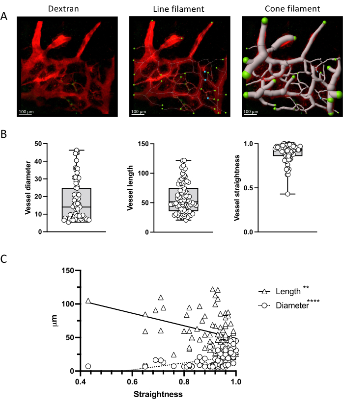
Figure 4: Vascular parameter quantification. (A) Measurement of vascular parameters via IMARIS filament tool in a representative z-projection of bone marrow vessels labeled with TRITC-dextran. Line and cone representations are shown. (B) Quantification of vessel parameters in the image shown in A. (C) Correlation between vascular parameters showing an opposite correlation between vessel straightness and length (negative, Spearman r = -3523; p < 0.0001; R² = 0.2102) vs diameter (positive; Spearman r = 0.4110; p < 0.0001; R² = 0.1299). Scale bars = 100 µm. Please click here to view a larger version of this figure.

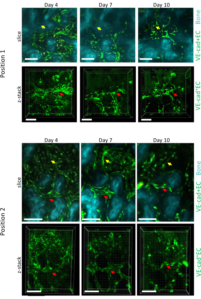
Figure 5: Longitudinal imaging of two different positions of the calvaria BM over AML development. Endothelial cells lining vessels are labeled with cdh5-GFP, bone surface with SHG, and macrophages in yellow (autofluorescence). Remodeling of preexisting vessels (red arrows) and formation of new vessels (yellow arrows) are shown. Scale bars = 100 µm. Please click here to view a larger version of this figure.

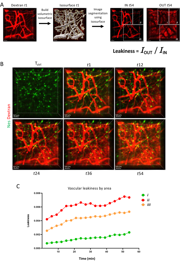
Figure 6: Vascular permeability. (A) Schematics of vascular permeability measurement via IMARIS surface tool. (B) Z-projection of the same area imaged longitudinally over 1 h. (C) Quantification of vascular permeability within areas as depicted in A. Please click here to view a larger version of this figure.

Supplemental Figure S1: Prepared skull. In the median plane, create an axis tangential to the calvaria, then save the prepared skull. Please click here to download this File.

Supplemental Figure S2: Plans 2 mm spaced. How to create a set of equally spaced planes (2 mm spacing) across the skull. Please click here to download this File.

Supplemental Figure S3: Observable surface contour. Create a sketch in the calvarial plane and create a pear-shaped spline from AP +6.5 to -2, 6 mm width at AP 0.0. Please click here to download this File.

Supplemental Figure S4: Observation vindow. Create a sketch in the calvarial plane and draw a 0.5 mm-thick C shape connecting to the Observation window. Please click here to download this File.

Supplemental Figure S5: Click new study. Navigate to the Simulation tab (if visible) or go to Simulation | Study. In the Study dialog box, choose Static as the study type. Click OK to create the new study. Please click here to download this File.

Supplemental Figure S6: Right click to create mesh. Refine the mesh in areas where high stress or deformation is expected. Please click here to download this File.

Discussion

The primary strength of intravital microscopy is its ability to capture dynamic cellular processes in real-time within their native environment, overcoming the limitations of traditional histological and ex vivo imaging methods. By directly observing the calvarial BM using the advanced imaging techniques coupled with fluorescent labeling as described in this protocol, researchers can study not only vascular functional parameters^8,14, but also longitudinal processes such as leukemic cell engraftment and migration^6,15, proliferation, and metabolic activity^16,17 preserving physiological relevance and avoiding artifacts associated with tissue fixation and processing.

The advantages of the BM calvaria intravital imaging over alternative bone sites include easy accessibility, transparency of the skull bone allowing for better visualization without bone damage, stability of the calvarium bone minimizing tissue motion artifacts, and reproducibility across experimental animals facilitating comparison between different experimental groups. The possibility to recover the animals and perform longitudinal imaging allows as well to reduce the number of animals used in a study. It is worth mentioning that because strain-specific differences in skull vessel growth patterns and consequent osteogenesis have been observed¹⁸, it is important to take this into account when designing the specific imaging implant for the desired mouse strain to allow perfect anatomical compatibility and access to the desired imaging site.

Another important point to mention is the potential differences in vascular and hematopoietic properties within the calvarial BM compared to other bones, a poorly explored question until recent years. Novel studies suggest localized functions for different bones, with the calvarial BM differing from other bones in terms of hematopoiesis, bone and vascular structure and function^{19,20,21,22,23}, as well as response to neurological pathologies²⁴. These differences need to be further explored and taken into account before generalizing specific calvaria findings.

The design and construction of an imaging implant is a key step for this experimental setup, starting from the choice of the material. Biocompatible implants play a pivotal role in biomedical research, facilitating a wide array of applications ranging from tissue engineering and regenerative medicine to drug delivery systems and in vivo monitoring devices. The choice of material for a head implant adapted for intravital imaging is critical. Ideally, the material should exhibit excellent biocompatibility, mechanical properties suitable for ensuring minimal flexibility and overall stability, and finally, the ability to integrate within the skull without inducing inflammation. Titanium is ideal for its good tolerability within the animal body, without induction of adverse reactions in contact with biological tissues, as well as for its resistance to corrosion, ensuring long-term stability even if exposed to body fluids or experimental solutions. Moreover, its mechanical strength makes it resistant to deformation and fracture. Despite its strength, titanium has a relatively low density, resulting in lightweight intravital imaging devices that minimize the burden on experimental animals and researchers. Finally, its versatility in fabrication allows for the customization of intravital imaging devices to suit specific experimental requirements, such as size, shape, and functionality.

Here, we designed a biocompatible head fixation implant using parametric modeling CAD software with built-in Finite Element Analysis (FEA) capabilities, specifically SolidWorks. This approach enables precise, iterative adjustments to the implant's structural and spatial requirements, ensuring both anatomical compatibility and mechanical resilience. Free alternatives, such as FreeCAD, offer similar modeling and simulation functionalities. The primary inputs for the design process include a high-resolution anatomical model of the mouse skull, a model of the microscope objective, and a model of the fixation system, which together inform the implant's dimensions and configuration. The final output is a platform-independent mesh file, typically in STL or STEP format, compatible with most 3D printing software.

The initial step involves capturing detailed anatomical features of the mouse's head using high-resolution imaging techniques, such as in vivo micro-CT scanning. This approach provides the highest anatomical detail and accuracy, capturing the skull's microstructures. 3D Scanning of a Prepared, Naked Skull could be also an option. This method, using laser or structured light scanners, is commonly employed on a prepared skull and provides accurate surface contours, though with less internal detail compared to micro-CT. Otherwise, anatomy models can be downloaded from open source publications and databases²⁵ or DigiMorph {https://www.digimorph.org/specimens/Mus_musculus/}. While convenient, these models may lack specimen-specific details, so adjustments are often needed for the specific animal in the study such as scaling to actual Bregma-Lambda distance. The acquired data are then used to create a precise 3D model of the mouse's skull, serving as the foundational template for the implant design.

To secure the implant onto the skull, a cementing structure is designed to cover the remaining skull surface not occupied by the observation window. This structure must provide robust attachment points while avoiding critical anatomical features. The cementing structure has multiple openings to ensure optimal polymerization of the cement under the implant through diffusion. Additionally, the walls of the cementing structure have a small draft angle, which allows the cement to anchor securely against these angled walls. The tail of the implant, which extends from the main body to the fixation system, is designed. This component is crucial for aligning and stabilizing the implant during observation, and its design must consider the available space and the anatomical constraints of the mouse's head. Finally, a dovetail mechanism is integrated into the implant design for easy attachment and detachment of the implant from the fixation system. This feature enhances the practicality and usability of the implant during repeated observations. The dovetail mechanism provides repeatable fixation for easy retrieval of observed tissues for repeated imaging sessions.

Readers considering the adoption of intravital microscopy imaging of the calvarial BM should carefully evaluate their research goals and experimental requirements to determine whether this method is appropriate for their studies. While intravital microscopy offers unparalleled insights into hematopoiesis, tissue microenvironment regulation, and vascular dynamics in vivo, it also presents certain technical challenges and limitations. Researchers should be prepared to address these challenges through careful experimental design, optimization of imaging parameters, and utilization of appropriate controls. Additionally, researchers should consider the availability of specialized imaging equipment, expertise in fluorescent labeling techniques, and computational resources for image analysis. Overall, intravital microscopy imaging of the calvarial BM holds tremendous potential for advancing our understanding of hematopoiesis and vascular biology, offering a unique window into the dynamic processes occurring within the BM microenvironment.

Materials

List of materials used in this article

Name	Company	Catalog Number	Comments
Amira	Thermo ScientificTM
Anesthesia			Isoflurane 2% to 3%
Anesthesic mask (animal detection)	Minerve
Anesthesic unit	Minerve
B6.Cg-Gt(ROSA)26Sortm9(CAG-tdTomato)Hze	Jackson laboratories	MGI:3809523
CalvariaVue	Ymetry	https://ymetry.com/site/head-fixation-implants/44-mouse-head-fixation-implant-for-calvaria.html
Dental cement	Kemdent	SUN527
Dextran 500 kDa-Cy5	Tebu-bio	DX500-S5-1	3 mg/mouse
Dextran 70 kDa-TRITC	Sigma	T1162	3 mg/mouse
Disinfectant	MP-Labo	Dermidine-60ml
Electric razor	Aescular	Isis
Eye gel	Ocry-gel	10g
Fiji	https://imagej.net/software/fiji/downloads	v 17 May 30
Fiji plugings to bridge with Imaris	https://imagej.net/software/fiji/downloads	Imaris_Bridge96.jar ; ImarisBridgeUtils.jar
Heating box	Datesand	Thermacage
Heating pad for surgery	Minerve
Imaging heating pad & rectal probe	F. Haer
Imaris v9.6.0	Oxford instruments
Intrasite gel	Chinoxia	2390766
LAS AF Software	Leica	LAS X 3.5.7.23225
Medication			Buprecare, 0.01 mg/kg
Objective HCX IRAPO L 25x/0.95 WATER	Leica	506374
Saline buffer (PBS 1x)	Sigma	P4417	Sterilize by autoclave
SP8 DIVE FALCON Multiphoton Microscope	Leica
Stereotoxic mask	Minerve	1201261
Sterilizator beads	Sigma	Z742555
Surgery tools	Moria	4877A; 2183
Survival blanket	SECURIMED	11006
Swabs / Tissues			Sterilize by autoclave
Syringe 1 mL 26 G	BD Plastipak	305501
Temperature controller	F. Haer	40-90-5D-02
Tg(Nes-EGFP)33Enik mice	Jackson laboratories	MGI:5523870
Tg(Pdgfb-icre/ERT2)1Frut mice	Jackson laboratories	MGI:3793852
Tg(Cdh5-cre/ERT2)1Rha mice	Jackson laboratories	MGI:3848982
Ultrasound gel	Parker laboratories	Aquasonic 100

References

- Lo Celso, C., et al. Live-animal tracking of individual haematopoietic stem/progenitor cells in their niche. Nature. 457 (7225), 92-96 (2009).
- Pittet, M. J., Weissleder, R. Intravital imaging. Cell. 147 (5), 983-991 (2011).
- Itkin, T., et al. Distinct bone marrow blood vessels differentially regulate haematopoiesis. Nature. 532 (7599), 323-328 (2016).
- Christodoulou, C., et al. Live-animal imaging of native haematopoietic stem and progenitor cells. Nature. 578 (7794), 278-283 (2020).
- Upadhaya, S., et al. Intravital imaging reveals motility of adult hematopoietic stem cells in the bone marrow niche. Cell Stem Cell. 27 (2), 336-345.e4 (2020).
- Hawkins, E. D., et al. T-cell acute leukaemia exhibits dynamic interactions with bone marrow microenvironments. Nature. 538 (7626), 518-522 (2016).
- Duarte, D., et al. Defining the in vivo characteristics of acute myeloid leukemia cells behavior by intravital imaging. Immunol Cell Biol. 97 (2), 229-235 (2019).
- Passaro, D., et al. Increased vascular permeability in the bone marrow microenvironment contributes to disease progression and drug response in acute myeloid leukemia. Cancer Cell. 32 (3), 324-341.e6 (2017).
- Jia, Y., et al. FLT3 inhibitors upregulate CXCR4 and E-selectin ligands via ERK suppression in AML cells and CXCR4/E-selectin inhibition enhances anti-leukemia efficacy of FLT3-targeted therapy in AML. Leukemia. 37 (6), 1379-1383 (2023).
- Pendleton, E. G., Tehrani, K. F., Barrow, R. P., Mortensen, L. J. Second harmonic generation characterization of collagen in whole bone. Biomed Opt Express. 11 (8), 4379-4396 (2020).
- Dispositif de liaison d'un animal de laboratoire à au moins un système d'expérimentation, et procédé de fixation d'un tel dispositif. France patent. , WO/2021/123449 (2021).
- Horton, S. J., et al. Acute myeloid leukemia induced by MLL-ENL is cured by oncogene ablation despite acquisition of complex genetic abnormalities. Blood. 113 (20), 4922-4929 (2009).
- Scott, M. K., Akinduro, O., Lo Celso, C. In vivo 4-dimensional tracking of hematopoietic stem and progenitor cells in adult mouse calvarial bone marrow. J Vis Exp. (91), e51683(2014).
- Jung, Y., et al. Intravital imaging of mouse bone marrow: Hemodynamics and vascular permeability. Methods Mol Biol. 1763, 11-22 (2018).
- Le, V. H., et al. In vivo longitudinal visualization of bone marrow engraftment process in mouse calvaria using two-photon microscopy. Sci Rep. 7, 44097(2017).
- Spencer, J. A., et al. Direct measurement of local oxygen concentration in the bone marrow of live animals. Nature. 508 (7495), 269-273 (2014).
- Yang, M., Mahanty, A., Jin, C., Wong, A. N. N., Yoo, J. S. Label-free metabolic imaging for sensitive and robust monitoring of anti-CD47 immunotherapy response in triple-negative breast cancer. J Immunother Cancer. 10 (9), e005199(2022).
- Li, W., et al. Tracking strain-specific morphogenesis and angiogenesis of murine calvaria with large-scale optoacoustic and Ultrasound Microscopy. J Bone Miner Res. 37 (5), 1032-1043 (2022).
- Lassailly, F., Foster, K., Lopez-Onieva, L., Currie, E., Bonnet, D. Multimodal imaging reveals structural and functional heterogeneity in different bone marrow compartments: functional implications on hematopoietic stem cells. Blood. 122 (10), 1730-1740 (2013).
- Rindone, A. N., et al. Quantitative 3D imaging of the cranial microvascular environment at single-cell resolution. Nat Commun. 12 (1), 6219(2021).
- Mills, W. A. 3rd, Coburn, M. A., Eyo, U. B. The emergence of the calvarial hematopoietic niche in health and disease. Immunol Rev. 311 (1), 26-38 (2022).
- Bixel, M. G., et al. Angiogenesis is uncoupled from osteogenesis during calvarial bone regeneration. Nat Commun. 15 (1), 4575(2024).
- Koh, B. I., et al. Adult skull bone marrow is an expanding and resilient haematopoietic reservoir. Nature. 636 (8041), 172-181 (2024).
- Kolabas, Z. I., et al. Distinct molecular profiles of skull bone marrow in health and neurological disorders. Cell. 186 (17), 3706-3725.e9 (2023).
- Rosenhain, S., et al. A preclinical micro-computed tomography database including 3D whole body organ segmentations. Sci Data. 5, 180294(2018).
Reprints and Permissions