Mechanical Mapping of Spheroids Using Brillouin Spectroscopy

Summary

This article describes a protocol for mechanical characterisation of living spheroids within a 3D matrix using Brillouin micro-spectroscopy. This all-optical method enables spheroid visualisation with microscale resolution and quantitative mechanical properties. This approach has implications for mechanical phenotyping; for instance, determining pathological states of tumor spheroids within a 3D microenvironment.

Abstract

Brillouin spectroscopy, an emerging technique gaining significant interest in biomedical science, allows researchers to gather information related to mechanics and structure by interrogating the viscoelastic and architectural properties of specimens in a non-destructive, contact-free manner. This approach evaluates the mechanical properties of 3D samples by measuring the interaction of visible light with thermally induced acoustic waves/phonons. The information that Brillouin spectroscopy provides has potential for in vivo assessment of biophysics and potential diagnosis of disease pathologies. A significant advantage of Brillouin spectroscopy is the capability to assess microscale mechanics inside a biological sample; other conventional techniques that can achieve this resolution, such as atomic force microscopy, can only probe samples in 2D since they require direct contact. This work describes the application of Brillouin micro-spectroscopy to investigate the biomechanics of living spheroids embedded within a 3D hydrogel matrix. Encapsulation of cellular spheroids within a 3D microenvironment establishes a spheroid system that closely recapitulates the interface between cells and the extracellular matrix in vivo. In our protocol, we describe spheroid sample preparation and measurements of Brillouin spectra with sequential fluorescence imaging. Additionally, we discuss procedures for spectral data analysis and technical details about the optical system.

Introduction

Culturing cells in 3D models is advantageous compared to the typical 2D cell culture methods, as it better recapitulates tissue structures and cell-cell interactions found in vivo. Spheroids are 3D cell aggregates that facilitate complex cell-cell interactions; these interactions are compromised in cells grown as a monolayer on tissue culture plastic. Spheroids can be grown within a scaffold that mimics the microenvironment where the cell originated from. For example, hydrogels are a popular biomaterial used to culture cells/spheroids in as they allow precise control of parameters such as stiffness, degradability, pore size, and the incorporation of growth factors¹ (Figure 1A). Mechanical cues often precede biochemical changes in disease pathologies such as cancer and fibrosis^2,3, therefore, acquiring the biomechanical signature in clinically relevant 3D models of disease is instrumental for developing diagnostic interventions to inform therapeutic practice and understanding the underlying pathophysiology⁴.

Brillouin Microscopy (BM) is an imaging technique that allows the mechanical properties of biological materials to be measured in 2D planes^5,6,7. BM has some key advantages over other more commonly used methods, such as atomic force microscopy (AFM) and elastography. It is well-documented that AFM can achieve high spatiotemporal mechanical resolution and that elastography can probe mechanics inside samples^8,9 . BM does not require direct contact with the material under investigation, making it an ideal technique over AFM for samples/cells that are difficult to access, such as spheroids within hydrogels. Another key advantage of BM is that it does not require labelling of samples and can provide microscale resolution inside biological samples, which commonly used elastography methods cannot achieve⁷; more advanced optical elastography techniques can operate at microscale resolution¹⁰. It should be noted that the precise effective resolution in Brillouin imaging of heterogeneous biological samples is not trivial to define. Firstly, for a given illumination wavelength, it depends on the optical properties describing the focal spot size (numerical aperture, NA, of the objective lens and sample opacity). Additionally, the accuracy with which the mechanical properties of the sample can be probed, as well as the shape of the Brillouin spectrum, is influenced by the acoustic characteristics of the material (phonon wavelength and propagation length)^11,12. The underlying phenomenon behind Brillouin spectroscopy is Brillouin scattering, where the incident monochromatic laser light interacts with spontaneous, thermally induced acoustic phonons within the biological medium. This results in inelastic scattering of light and (Brillouin frequency shift, BFS) in Figure 1B and is typically in the order of several GHz and depending on whether the photon loses, or gains energy, Brillouin Stokes and anti-Stokes peaks are detected in the spectrum of the scattered light, respectively. Through its dependence on the local sound velocity in the medium, the BFS is related to the elastic longitudinal modulus, which is in turn empirically correlated to the Young's modulus^7,13; however, care must be taken when making comparisons between these moduli as (i) they are not directly related to each other, (ii) Young's modulus is usually in the Pa-kPa range for biological samples and soft matter whereas the longitudinal modulus obtained from Brillouin is in GPa range, and (iii) parameters such as refractive index changes and material density must be taken into account⁷. The Brillouin linewidth (in Figure 1B) is another measure obtained from BM. It is related to the longitudinal loss modulus, giving insights into the viscosity of the sample; these properties can be correlated with viscoelasticity¹⁴. Thus, BM allows for the assessment of the viscoelastic properties, where a larger BFS implies a stiffer material, and a larger linewidth implies a more viscous material (Figure 1B). It should be noted that elastic (Rayleigh) scattering, where the photons do not undergo a frequency shift, has a significantly larger likelihood of occurring compared to Brillouin scattering. Therefore, Brillouin spectrometers must be equipped to suppress the Rayleigh signal.

BM has been used to characterize the mechanical properties of various tissues, biomaterials, and 3D cell culture models. For example, BM was utilized to differentiate between melanoma and the surrounding healthy tissue, showing that the non-cancerous tissue was significantly softer than the melanoma¹⁵. Rad et al. showed that increasing the polymer concentration of hydrogels resulted in increased BFS and linewidth. At the lowest polymer concentrations, hydrogels with cells showed larger decreases in Brillouin frequency shifts over seven days compared to empty hydrogels, which was proposed to be due to cellular remodeling of the hydrogel. This was not observed at 10% polymer concentration, which underscored a possible lack of cell viability found in these hydrogels¹⁶.

Of most relevance to the present study, BM has been used to investigate the mechanical properties of spheroids^17,18,19,20. In particular, the effect of the local microenvironment on spheroid mechanics can be detected using BM²⁰. Compared to tumor spheroids cultured in compliant hydrogels, spheroids grown in stiff hydrogels exhibited a higher BFS, which is indicative of an increased elastic modulus²⁰. Spatial variation of mechanical properties within a spheroid can also be characterized with BM. For example, the BFS of tumor spheroids has been found to increase towards the spheroid core^20,21. Furthermore, a decrease in BFS correlates with increased invasiveness of tumor spheroids²⁰. BM has been used to investigate the mechanical changes of tumor spheroids in response to osmotic shock²². In the study, spheroid growth was monitored over 5 days, finding that the initial mechanical differences between cancer and healthy spheroids observed with BM were lost with time. Another study found an increase in BFS of the spheroid after 7 days which was attributed to increasing spheroid size and number of cells¹⁶.

Furthermore, multimodal investigations, employing Brillouin microscopy alongside AFM and rheology, have been carried out to probe the mechanical properties of cells and hydrogels^16,23,24. Rad et al. used rheology to contextualize the trends measured with BM, establishing a strong positive correlation between the longitudinal modulus and storage shear modulus with respect to the polymer concentration of hydrogels¹⁶. Brillouin microscopy and optical tweezer micro-rheology were used to measure the mechanics of cancer cells cultured in 3D hydrogels²³. In this study, decreased mechanical heterogeneity was found among cells in spheroids compared to single cells grown suspended in hydrogels.

In this work, a protocol to investigate the mechanical properties of live spheroids embedded in hydrogels with a commercial Brillouin microscope is detailed (Figure 1). Berghaus et al. described a protocol detailing the steps to build a high-resolution Brillouin spectrometer and a method to calibrate it with reference materials²⁵. Further, a protocol by Shi et al. describes the use of Brillouin microscopy to monitor the changes in the mechanical properties of embryonic tissue²⁶. We use mesenchymal stem cell (MSCs) spheroids in poly(ethylene) glycol (PEG)-maleimide hydrogels to mimic the bone marrow niche and investigate the mechanical properties of this environment. This 3D model has the potential to uncover the mechanical signature of bone marrow diseases, including leukemia, multiple myeloma, and secondary bone cancer. The protocol is therefore directly transferable to 3D models of other diseases where disrupted mechanobiology may have an important role in the pathology. The spheroid and hydrogel preparation, fluorescence imaging, and Brillouin microscopy techniques are detailed. The recommended procedures, possible drawbacks, and potential improvements of the technique are discussed. The detailed experimental setup description is presented in Figure S1 and within the Supplementary Materials and methods section related to the experimental setup.

Protocol

1. 2D cell culture

NOTE: Where possible, ensure that all cell culture work is performed in a sterile environment using a tissue culture standard laminar flow hood to avoid contamination. MSCs were used in the present protocol, but other cell types can be utilized to create spheroids, depending on the specific aims of the study.

1. Culture MSCs in Dulbecco's Modified Eagle Medium (DMEM) cell culture medium, with sufficient volume to cover the cells, containing 4.5 g/L D-Glucose, + L-Glutamine supplemented with 10% fetal bovine serum (FBS), 100 µM sodium pyruvate, 1% non-essential amino acids (NEAA), 1% penicillin and streptomycin. Incubate cells at 37 °C and 5% CO₂.
2. Passage cells at 70-80% confluency, by incubating with 0.05% trypsin ethylenediaminetetraacetic acid (EDTA) (the volume of trypsin added should be 1/3 of the DMEM volume) for 3 min at 37 °C and 5% CO₂ to detach cells from the plate. To stop the reaction, add culture media containing FBS (at least matching the volume of added trypsin). Count cells using a haemocytometer.

2. Spheroids preparation

NOTE: Where possible, ensure that all cell culture work is performed in a sterile environment using a tissue culture standard laminar flow hood to avoid contamination. In this study, microwell plates were used to create MSC spheroids. These plates are comprised of 24 wells, and each well contains 1200 microwells, 400 µm in diameter. This allows the preparation of a large number of spheroids (Figure 2).

1. To prepare the microwell plate, pre-treat the wells by adding 500 µL of anti-adherence rinsing solution to each well. Centrifuge plate at 1,300 g for 5 min at room temperature. Under a microscope at 20x magnification, check whether there are any air bubbles present. If there are, repeat the centrifugation step. Remove the anti-adherence rinsing solution.
2. To wash the plate, add 1 mL of phosphate-buffered saline (PBS) and aspirate. Do this twice to ensure the rinsing solution has been completely removed.
3. Determine the number of cells per spheroid and the number of spheroids per gel. This will depend on individual research questions. For example, we used 100 cells per spheroid and 100 spheroids per gel. Therefore, for this protocol, only one well of the microwell plate was required, as this creates 1200 spheroids in total. To calculate the number of cells required for one well, we did the following calculation: 1200 x 100 = 1.2 x 10⁵. Calculate the volume of cell suspension containing 1.2 x 10⁵ cells. Centrifuge the cell suspension at 300 g for 5 min at room temperature and remove supernatant.
4. Resuspend the cells in 1 mL of DMEM (+4.5 g/L D-Glucose, + L-Glutamine) supplemented with 100 µM sodium pyruvate, 1% NEAA, 1% penicillin and streptomycin. Add 1 mL of cell suspension to one well of the microwell plate and gently pipette up and down to disperse cells evenly throughout the well. Be careful not to introduce air bubbles. Centrifuge the plate at 100 g for 3 min at room temperature.
   NOTE: At this stage, we do not add FBS to the media. This is to prevent the cells from attaching to the tissue culture plastic.
5. Observe the plate under the microscope to ensure the cells are evenly distributed and have sunk to the bottom of the microwells. Incubate cells at 37 °C and 5% CO₂. Observe spheroid formation 24 h later.
   NOTE: Spheroids can be left in the plate for up to 48 h, depending on the cell type and desired compactness of the spheroid.
6. To harvest the spheroids from the plate, first slowly and gently remove the culture media, aiming not to disturb the spheroids. To prevent spheroids from sticking to plasticware, coat pipette tips and tubes using PBS with 1% FBS. To avoid the spheroids getting stuck in the pipette tips, cut the tip to widen the opening. Maximum recovery tips can be used during these steps as an extra measure to prevent the loss of spheroids. Add 500 µL of PBS to each well of the microwell plate and pipette up and down to dislodge spheroids. Collect the PBS with suspended spheroids in a tube (Figure 2).
7. View the plate under the microscope at 20x magnification and repeat this step until most of the spheroids have been successfully removed.
8. To count the number of spheroids in the suspension, transfer 50 µL from the suspension into a well of a 96-well plate. Count the number of spheroids in the 50 µL. To aid counting, a cross can be drawn on the bottom of the well using a permanent marker. Calculate the number of spheroids using equation (1):
   

3. Preparation of PEG hydrogels

NOTE: Where possible, ensure that all cell culture work is performed in a sterile environment using a tissue culture standard laminar flow hood to avoid contamination. In this study, PEG-maleimide hydrogels were used, but other types can also be utilized. PEG-maleimide hydrogels were formed using the thiol-Michael addition reaction²⁷. The crosslinkers used were a mixture of PEG-dithiol and protease-degradable peptide, flanked by two cysteine residues (VPM peptide, GCRDVPMSMRGGDRCG). The gels in the present study used 70% PEG-dithiol and 30% degradable VPM peptide.

1. Make a 200 mg/mL stock solution of VPM peptide and add 2.4 µL of peptide per gel. Make a 200 mg/mL stock solution of PEG-dithiol and add 5.6 µL per gel.
2. Resuspend the spheroids in PBS before mixing with the crosslinkers (Figure 2). Mix the spheroid suspension with the PEG-dithiol (5.6 µL per gel) and VPM (2.4 µL per gel). This solution is termed Solution B.
   NOTE: In this protocol, 100 spheroids were added per gel.
3. Make a 250 mg/mL PEG-Maleimide stock solution. Add 50 µg of fibronectin per gel. Mix the PEG-Maleimide and fibronectin solution; this is termed Solution A. Pipette Solution A (40.3 µL for 100 µL gels) onto the bottom of a 12-well tissue culture plate. Add Solution B (59.7 µL for 100 µL gels) at a molar ratio 1:1 maleimide:thiol to ensure full crosslinking; ensure that gelation occurs instantaneously. The final volume of the hydrogels is 100 µL.
4. Incubate gels for 30 min at 37 °C and 5% CO₂ to allow gelation. Add complete culture media (DMEM supplemented with 10% FBS, 100 µM sodium pyruvate, 1% NEAA, and 1% penicillin and streptomycin) to the well, ensuring the gel is fully submerged (Figure 2). Incubate the gel at 37 °C and 5% CO₂ until ready to take measurements under the Brillouin microscope.
   NOTE: The duration of spheroid culture within the hydrogels prior to Brillouin measurements will be dependent on the cell type and the research question. For example, in this study, the spheroids are typically cultured within hydrogels for up to 7 days, during which the spheroids are monitored by Brillouin microscopy. Viscoelastic properties of the hydrogels with/without spheroid encapsulation were characterized and show no significant impact of spheroids on gel mechanics (Figure S2).

4. Fluorescence staining and imaging of spheroids in hydrogels

NOTE: In this study, cell nuclei and actin filaments comprising the cytoskeleton were fluorescently stained and imaged prior to Brillouin measurements.

1. To stain actin, add live actin stain to culture media at 1 in 500 dilution 3 h before imaging. Keep the sample out of light by wrapping in foil. Incubate the gel at 37 °C and 5% CO₂.
2. To stain the nuclei, add 2 drops/mL of live nuclear stain to the culture media surrounding the gel 40 min before imaging. Return the samples to the incubator.
3. Acquire fluorescence images as soon as possible after the staining incubation time is complete. Verify that the appropriate optical path (exposing the microscope camera) and the correct filter wheel position are selected. Dim the lights in the room and capture the background. Switch on the light-emitting diode (LED) light source and choose the wavelength depending on the staining protocol (here, 385 nm was used for nuclei and 621 nm for actin imaging). Acquire fluorescent images of spheroids at 20x magnification with preferred software. Turn off the LED source when finished.

5. Brillouin microscopy of spheroids

1. Switching on the devices and laser emission
   1. Switch on the devices: the computer, spectrometer, microscope cameras, the microscope, the laser cooling fan, and laser emission by turning on the key on the controller. Ensure that this is done 15 min prior to spectrometer optimization to ensure the laser has thermalized. Verify that the emitted laser power is as expected with a power meter (100 mW in our experiment).
2. Turn on the temperature-control application (see Table of Materials) and verify that the etalon temperature is optimized by measuring the beam power after the etalon. If it is significantly lower than expected (after accounting for the optical density (OD) filter used), change the target temperature by 1 °C and observe if there is an increase in power with time. If there is a decrease, reverse the direction of change. Once the power is close to expected, tune by small increments (0.1 °C) until the maximum is reached.
3. Setting the objective lens focal spot inside the acrylic cube
   NOTE: Suppression of elastic scattering and coupling from the "pump killer" to the spectrometer is optimized with a sample of stiff, homogenous reference material prior to each experiment. In this study, an acrylic cube is used.
4. Open SpectraLok software and wait until all devices are detected. On the left side of the main window (Figure 3), select the spectrometer camera.
   1. Install the acrylic cube on the microscope sample holder with the clear side facing the objective lens. Lower the objective lens as much as possible and center the cube under it. Ensure that the optical path in the microscope is chosen so that the spectrometer camera is exposed (set the rotary port selector to L).
      NOTE: In our setup, the L port is connected to the confocal circulator, while R is connected to the microscope camera port.
   2. In the SpectraLok Camera window, set the sensor exposure time to 500 ms and the software gain to 100. The software gain setting only enhances the contrast for visualization purposes.
5. Unblock the laser shutter.
   NOTE: As the laser emission is on, take care to never put head/eyes in the laser beam path.
   1. Press capture, and move the objective lens upwards. There will be a significant increase in signal intensity, and a saturated pattern (Figure 4A) will appear. This is caused by a strong reflection of laser light at the air-acrylic cube interface. Moving the lens further up, the signal intensity will decrease, and Brillouin peaks will become apparent. Continue repositioning the objective lens until the intensity of the Brillouin peaks is constant (Figure 4B). This corresponds to the focal spot located entirely within the acrylic cube.
6. Optimizing the etalon pressure to minimize residual elastically scattered light
   NOTE: The purpose of the following steps is to suppress the elastically scattered Rayleigh signal so that only the frequency-shifted Brillouin light reaches the spectrometer camera.
7. In SpectraLok software, open the Pump Killer (PK) control window (Figure 5).
8. Zoom in on one of the brightest Brillouin orders and adjust the pressure actuator position in increments of 100 µm by clicking move rel to minimize the Rayleigh peak intensity. If the Rayleigh signal is increasing, reverse the direction of change by clicking reverse. Subsequently, fine-tune the etalon pressure in increments of 10 µm.
   NOTE: In the acrylic cube, the Rayleigh light can be completely suppressed; this may not be the case in a heterogeneous biological sample.
9. Optimizing the stripe overlay to "unwrap" spectral data
   NOTE: The following procedure ensures that the (x, y) pixel coordinates of the camera sensor are appropriately mapped to wavelength via application of the look up table LUT.
10. In the camera window, zoom in on one of the Brillouin orders.
11. Press s to visualize stripes across which the LUT is applied on the camera image (Figure 6A). Open the Settings window and press quick calibrate to recalculate the optimal horizontal offset of the stripes. If the sensor is saturated, reduce the exposure time before this step.
    1. In the camera window, verify that the purple stripes are well overlaid with the central region of Brillouin peaks (Figure 6B).
12. Optimizing the PK-spectrometer coupling
13. Adjustment of the collimator lens axes allows maximizing the efficiency of the coupling of light from the PK to the spectrometer.
14. Open the spectrum window and click unwrap to retrieve the spectrum (Figure 7).
15. Open the PK control window. With increments of 0.0005°, iteratively adjust the collimator axes 1 and 2 to maximize the Brillouin signal. If needed, the etalon pressure control can be further optimized. In a homogenous acrylic cube, the Rayleigh signal can be completely suppressed (Figure 7A). While accurate Brillouin measurements with some residual Rayleigh signal are feasible (Figure 7B), in cases of poor suppression (Figure 7C), elastically scattered light obscures the Brillouin signal.
16. Verify that the achieved Brillouin signal is comparable to reference amplitude. For example, in our system, at exposure of 500 ms and with OD 0.3 the Brillouin peak intensity amplitude is approximately 3000 counts. To save changes of the PK parameters to the configuration file, in the PK window, click refresh all and save all. Furthermore, in the main window, press save in the File I/O section.
17. Switching to scanning software and verifying that the parameters are still optimized
18. Close SpectraLok and open the scanning software. In the present protocol, LabVIEW-based software was used and is described in more detail in Figure S3. To set the scan geometry, this proprietary user interface (UI) is used to control the Prior XY-Z translation stage; however, other methods can be employed.
    1. Install the glass-bottom petri dish with the hydrogel-spheroid sample instead of the acrylic cube (Figure 8). To prevent dehydration of the gel, the incubator is set at 37 °C and 95% relative humidity. Remove the petri dish lid and add media to submerge the gel. Add a coverslip to the top of the gel to prevent movement of the gel.
    2. Locate the spheroid. With the laser beam blocked, switch the microscope optical path to the eyepiece. Turn on the white light illumination. Using the joystick, manually control the sample stage, locate and focus on the spheroid.
    3. Acquire a brightfield image of the spheroid. Adjust the illumination brightness by rotating the control wheel. Set the optical path to R, thus exposing the microscope camera. Exposure time can be adjusted as needed to obtain a high contrast image (i.e., 50 ms).
    4. Verify that the spectrometer and unwrapping parameters are still optimized. Set the microscope port to L and capture the background with the laser blocked. Unblock the laser by turning the wheel to firing. Based on the desired signal-to-noise ratio, select the exposure time. Exposure time typical to these measurements is 200-500 ms.
    5. If some time has passed (i.e., several hours) since initial calibration or there has been a mechanical disturbance of the system, the etalon pressure setting or the PK-spectrometer coupling may no longer be optimal. Repeat steps 5.3-5.5 to re-optimize the aforementioned, if necessary.
    6. From the unwrapped spectrum, select the Brillouin peak fitting range. Adjust the threshold value to about half the intensity of the Brillouin peaks. Disregard the Brillouin peaks with amplitude below this threshold. Correct the laser wavelength according to all of the identified Brillouin peak pairs.
19. Setting the multi-dimensional scan geometry
20. Choose the raster scan geometry by adjusting the width of the scan region and the step size.
    NOTE: For spheroids of size approximately 70 µm, for a low-resolution scan, we typically use a scan area of 150 µm × 150 µm and a step size of 10 µm. This yields a low-resolution 2D map in approximately 3.4 min.
    1. Start the scan.
21. Switching off the Brillouin system
    1. Close the software and turn off the computer. Turn off the laser emission using the key on the controller. Leave the shutter wheel at the blocked position. Switch off the laser fan cooling. Turn off the microscope and spectrometer cameras. Finally, turn off the microscope.

Results

Files obtained after a scan include spectra, scan fitting parameters (.csv), scan parameters and analysis, BFS and linewidth maps, brightfield image with the scan region of interest identified, and a screenshot of the UI window. For each point of the multi-dimensional Brillouin scan a BFS value is acquired. In Figure 9, an example high-resolution scan is displayed alongside the brightfield image, and fluorescence images showing actin filaments and nuclei. Note that in our system, the fluorescence is used to guide the imaging and interpretation of the Brillouin maps, rather than for precise quantification, as the microscope is equipped with epi-fluorescence rather than a confocal imaging module. Here, the out-of-focus fluorescence of the sample impacts the effective resolution. Using the 2D Brillouin scan data and the brightfield image, as shown in Figure 9, the spheroid can be segmented, and an average BFS for the spheroid can be obtained. This can be compared to the average BFS of the gel. Segmentation can be facilitated with tools such as Fiji (ImageJ)²⁸ or Napari Python plug-in²⁹.

The spheroid is segmented with a simple Python software to batch process the data generated by the microscope's UI. The brightfield image is cropped to match the Brillouin scan region. The spheroid boundary is manually traced by the user, as shown in Figure 10B, to identify the spheroid area. This area is then down-sampled (Figure 10B, top right) to match the size of the corresponding low-resolution Brillouin shift map (Figure 10A). Due to the down-sampling, pixel values that are not 0 or 1, are said to be ambiguous (undetermined whether they belong to the spheroid or to the gel) and are conservatively excluded from further analysis (Figure 10B, bottom right). Binary masks for the spheroid and gel are then created and applied to retrieve BFS values for the gel (Figure 10C) and spheroid (Figure 10D). It should be noted that the softer outermost values of the spheroid map may correspond to the boundary and appear softer (green in Figure 10D). While the edges of the spheroid have been shown to be softer than the core²⁰, the lower BFS value can also be the result of the contribution of both the spheroid and the gel within the scattering volume to the Brillouin spectrum³⁰. To select the values that confidently fall within the spheroid and are free from potential gel contribution, means clustering was applied to the data in Figure 10D (the top right image shows the two regions detected). Optionally, it is checked whether these values are also from the outermost radial coordinate. If both conditions are satisfied, the identified boundary values are excluded from the calculation of the mean BFS for the spheroid (Figure 10E). In irregularly shaped spheroids, some values may not be correctly attributed to the boundary (if, for example, some part of the spheroid was outside the focal plane).

Note that in our typical experiments, we are interested in measuring the bulk BFS value of individual spheroids rather than cell-to-cell or region-to-region variation within the model. Coarse sampling helps to increase the experimental throughput and reduce scan duration. Furthermore, it is representative of the bulk properties of the spheroid, as the mean BFS value from the segmented high-resolution scan agrees with the value extracted from coarser measurements (Figure 11).

Validation of system sensitivity and measurement was carried out using a distilled water reference sample. Specifically, with ~15 mW average power at the focal plane and spectrometer camera exposure times of 50, 100, 250, 500, and 1000 ms, the standard deviations of the BFS distribution were 21, 14, 8, 6, and 5 MHz, respectively, as shown in Figure S4. The data were obtained from 441 repeated consecutive measurements at that exposure time.

In the context of the technique we have described in this protocol, these representative results highlight the robustness of the technique to acquire clearly resolved spheroid mechanics from living cells in parallel with live fluorescent staining of cell features. The segmentation approach in our representative analysis allows the user to accurately dissect the spheroid mechanics from the surrounding 3D hydrogel microenvironment. Collectively, this approach can couple biochemical and mechanical information to inform the user about comprehensive changes in cell phenotype and their surrounding environment between different experimental conditions; one could imagine, for instance, potential applications of this approach to comprehensively characterize patient-derived cells to determine their pathological state and inform clinical practice.

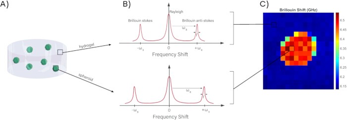
Figure 1: Fundamentals of Brillouin micro-spectroscopy. (A) Hydrogel with embedded spheroids. (B) The spectra of scattered light from the sample in (A) and denote BFS (ωB) and linewidth (Γ), respectively. Hydrogel yields a smaller BFS (top) than the spheroid (bottom). (C) Acquisition of multiple spectra to form a 2-dimensional BFS map. Please click here to view a larger version of this figure.

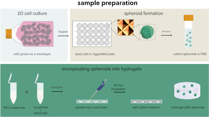
Figure 2: Schematic of sample preparation. Cells are grown as a monolayer prior to adding trypsin and culturing in microwell plates to create spheroids. After 24 h, the spheroids are collected in PBS. The spheroids are incorporated into PEG-maleimide hydrogels in the wells of a tissue culture plate. After 30 min, culture medium is added. Please click here to view a larger version of this figure.

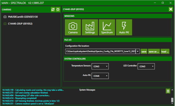
Figure 3: Main window of SpectraLok software. Please click here to view a larger version of this figure.

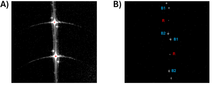
Figure 4: Spectrometer camera images. (A) Saturated signal at the air-acrylic interface and (B) Diffracted Brillouin orders from within the acrylic cube. B1, B2 are Brillouin peaks, R is residual elastically scattered Rayleigh light. Please click here to view a larger version of this figure.

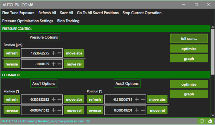
Figure 5: PK control window. Please click here to view a larger version of this figure.

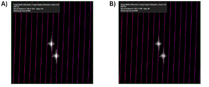
Figure 6: Stripe alignment in spectral data unwrapping. (A) Misaligned stripes in the camera window, and (B) optimal spectral data unwrapping is achieved when the LUT stripe overlay is centered across the Brillouin peaks. Please click here to view a larger version of this figure.

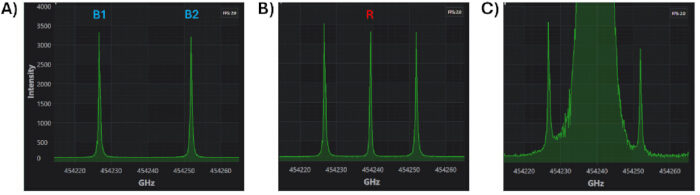
Figure 7: Unwrapped spectrum displaying the Brillouin peaks. (A) Rayleigh peak (R) completely and (B) partially suppressed. (C) The Rayleigh signal interferes with the measurement of the Brillouin spectrum (B1 and B2). Please click here to view a larger version of this figure.

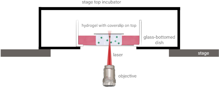
Figure 8: Sample setup for Brillouin microscopy. The hydrogel is placed in a glass-bottomed dish with the lid off and a coverslip placed on top so to prevent movement of the gel. The dish is placed in a stage top incubator which is positioned onto the microscope translation stage. Please click here to view a larger version of this figure.

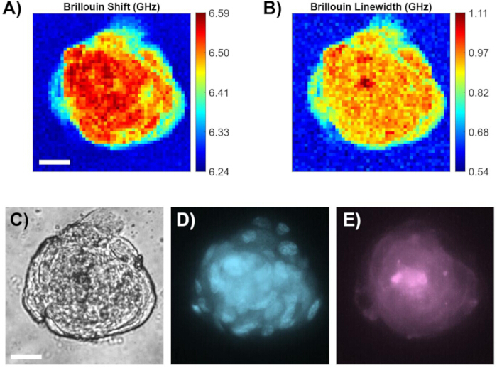
Figure 9: Representative images of a spheroid obtained in Brillouin, brightfield, and epifluorescence modalities. High resolution (A) BFS and (B) Brillouin Linewidth maps of an MSC spheroid in a hydrogel. (C) Brightfield and (D) epifluorescence images of nuclei and (E) actin filaments of the spheroid in the hydrogel. Scale bar (white) is 20 µm. Please click here to view a larger version of this figure.

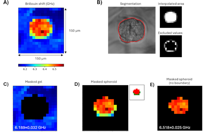
Figure 10: Example segmentation method. The low-resolution BFS map (A) is segmented into gel and spheroid regions. Tracing the spheroid contour in the brightfield image by the user (B) allows generating a down-sampled mask of the spheroid area, which is applied on the low-resolution BFS map. (C) The gel and (D) the masked spheroid are identified, with the latter further separated into boundary and central region, with means clustering (D, top right) and by checking the radial coordinate of the pixel. The values that confidently fall within (E) the central spheroid and (C) gel are used to calculate the mean BFS values. Please click here to view a larger version of this figure.

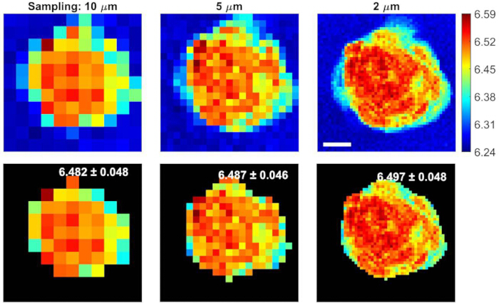
Figure 11: Comparison of BFS values obtained from maps with high and low spatial sampling. Coarse sampling is representative of the bulk mechanical properties of the spheroid. The difference in the mean Brillouin Shift value (top right corner of each image in the bottom row) of the segmented spheroid is negligible with 10, 5, and 2 µm sampling. The color bar denotes the Brillouin Shift values. Scale bar (white) is 20 µm. Please click here to view a larger version of this figure.

Supplementary File: Supplementary materials and methods. Please click here to download this File.

Discussion

We have established a protocol to use Brillouin microscopy for biomechanically imaging spheroids embedded in hydrogels with microscale resolution. The hydrogel can be distinguished from the live spheroid by differences in the BFS values obtained. In the representative results, we used MSC spheroids and PEG-maleimide hydrogels; however, this protocol is broadly applicable to other cell types (e.g., cancer cell lines). The cells in this study were imaged live and within a relevant 3D microenvironment, which demonstrates the feasibility of this platform in conjunction with biologically relevant models. Brillouin shift values for various ex vivo tissues such as the brain, muscle, skin, and cartilage from non-human species have been measured⁴. Brillouin microscopy has previously been effective at measuring in vivo tissue mechanics, for instance, the human lens and cornea³¹. The 3D microenvironments used in this protocol may contribute to the development of predictive tools for clinical applications, which will reduce the need for developing complex, expensive in vivo models going forward. The limitations of this protocol include spectral data analysis and interpretation, and ensuring cell viability with laser exposure.

Fluorescence imaging of live spheroids, showing the nuclei and actin filaments, highlights the ability to acquire molecular information to complement and contextualize the mechanical data. Actin is a key component of the cell cytoskeleton; these filaments are dynamic and able to respond to mechanical stress; therefore, it is of interest to visualize actin distribution alongside the viscoelastic properties of the cell³². Cell mechanical response to Latrunculin-A, a drug that inhibits the assembly of actin filaments, has been measured using Brillouin microscopy³³. The present protocol may be adapted to apply a stimulus or drug treatment to the sample to determine the corresponding effects on the organization of actin within the cells of the spheroid.

In this protocol, static measurements were made; however, measurements can be made over time in response to a variety of stimuli. In a recent study, the response of cells to a short-duration electrical impulse was measured in real-time using Brillouin microscopy, and subcellular changes in biomechanical properties were imaged³⁴. Although the bone marrow niche is the focus of the present study, the protocol can be adapted to investigate other diseases, such as cancer²⁰. Brillouin microscopy has been used to monitor drug efficacy in spheroids created with colorectal cancer cell lines, where differential changes in biomechanics of the spheroid rim to the spheroid core were found²¹. Although culturing cells as spheroids better replicates in vivo tissue architecture than conventional 2D cell culture, more intricate samples can be studied, like multicellular spheroids, organoids, and tissues^4,35. For example, live imaging by Brillouin microscopy of zebrafish larvae, mouse mammary gland organoids, and adult Caenorhabditis elegans was performed recently³⁵.

This protocol is a highly efficient approach to extract mechanical information from living cells in 3D. Commonly used approaches to derive cell mechanics, such as AFM, are limited to 2D samples and therefore incapable of accessing spheroids embedded within a 3D environment, which is much more physiologically relevant. Even at lower resolution scans, which can be completed on faster timescales, measurements are sufficient to distinguish cell mechanics from their surrounding environment. Additional coupling of fluorescence microscopy allows biochemical information to be simultaneously extracted from living specimens, which stand-alone Brillouin systems cannot achieve. Simple segmentation analysis, described in our method, allows a user-friendly approach to isolate spheroid mechanics from the overall mechanical map to gain specific insights into the cellular mechanics without interference from the surrounding environment.

It is essential to tune the temperature of the etalon (step 5.1.2) in the light source (Figure 1) to allow for maximum transmission of the central laser wavelength before each experiment. In day-to-day operation, as the laser is switched on, the wavelength may change slightly, decreasing the transmission available power output from 100 mW to a few mW. It should be noted that the optimum PK pressure setting to suppress elastically scattered light (Section 5.3) will also change; therefore, tuning the pressure before each experiment is also important. Note that if the discrepancy was significant, a full scan of the etalon pressure range can be facilitated to identify the suppression window (Figure 6, "full scan" and "graph").

Linear absorption of continuous-wave laser light may incur damage or changes to sample morphology and mechanical properties. This is particularly relevant in Brillouin micro-spectroscopy, where a low inelastic scattering cross-section implies a necessity for large excitation powers. Furthermore, during long high-resolution 2D Brillouin scans with higher NA objective lenses, the power density at the focal volume can impact the biochemical processes within the preparation³⁶. Ensure that the excitation beam is attenuated with optical density filters so long as a sufficient signal-to-noise ratio is achieved. Furthermore, the exposure time can be reduced. While long high-resolution Brillouin scans are more informative with respect to sample morphology, to determine the average BFS and linewidth of the spheroid versus the hydrogel, it is sufficient to take lower resolution scans of several minutes in duration. Alternatively, acquiring a high-resolution line profile (and the resulting BFS and linewidth) over the hydrogel-spheroid boundary can mitigate the scan time needed. This strategy has been used to determine cell thickness³⁰.

While not observed in low-resolution scans of several minutes, during long scans, the spheroid position may drift. Wrapping the sample petri dish in Parafilm or otherwise maintaining the relative humidity to prevent the dehydration of the hydrogel is recommended. Adhesive coatings to fix the hydrogel to the dish to ensure it remains stable during imaging have been used; for example, glass-bottom dishes can be treated with glutaraldehyde to allow for cell immobilization or material adhesion²³.

As described in steps 5.11-5.12, the spectral data and the corresponding Lorentzian fit results are retrieved from the LabVIEW-based UI. If needed, the acquired spectra can be de-noised in a custom user-implemented data analysis pipeline with, e.g., Savitzky-Golay filter, based on local least-squares polynomial fitting³⁷.

It should be noted that in virtually-imaged phase array (VIPA) spectrometers, the measured Brillouin peak linewidth is a convolution that includes the contribution of both the true experimental linewidth of the biological material and the inherent instrumental broadening of the spectrometer response (IRF). IRF can be measured from the full-width-at-half-maximum of the unbroadened Rayleigh peak (with the PK pressure setting reasonably off-suppression) and subtracted from the Brillouin linewidth, under the assumption that both the Brillouin peaks and the IRF are Lorentzians and their deconvolution is linear³⁸. Nevertheless, this can be assumed to be consistent with each measurement; thus, real biological trends in linewidth are not obscured if this subtraction is not carried out.

Another significant experimental parameter is the NA of the objective lens. As the axial extent of the optical point spread function scales with 1/NA³, higher NA allows imaging smaller structures. If the 6.5 µm focal spot spans two media, especially at their interface, the resulting Brillouin spectrum will include a contribution from both materials. This was utilized in Passeri et al.³⁰; however, ideally, the user may wish to avoid that or unmix the different components. Here, established approaches from fluorescence lifetime imaging (spectral phasor analysis³⁹) or Raman spectroscopy (principal component analysis⁴⁰) have been applied. These could potentially be applied to the spectra originating at the spheroid-hydrogel boundary. Importantly, as higher NA implies a wider light collection angle, a larger range of scattering wavevectors is collected. This leads to further broadening of the Brillouin peaks. Nevertheless, in back-scattering geometry (as in the present study), NA under 0.7 has been shown to have negligible effects. Furthermore, the minimal effect is systematic and consistent when the same objective lens is used⁴¹.

Materials

List of materials used in this article

Name	Company	Catalog Number	Comments
4-arm PEG-Maleimide (20 kDa)	Creative PEGWorks	PSB-455	https://creativepegworks.com/product/4-arm-peg-mal-mw-20k
AggreWell 400 plates	STEMCELL Technologies	34411	http://stemcell.com/products/aggrewell400.html
Air-spaced etalon	LightMachinery	HF-16074-660	https://lightmachinery.com/spectrometers/brillouin-spectroscopy-excitation-laser-optimization/
Anti-adherence rinsing solution	STEMCELL Technologies	7010	https://www.stemcell.com/products/aggrewell-rinsing-solution.html
Bold Line Top Stage Incubator	Okolab	H301-NIKON-NZ100/200/500-N	https://www.oko-lab.com/live-cell-imaging/stage-top-digital-gas/chamber/nikon/h301-nikon-nz100-200-500-n
Cobolt Flamenco-100 660 nm laser	Huebner	0660-05-01-0100-700	https://hubner-photonics.com/products/lasers/single-frequency-lasers/05-01-series/
Confocal circulator	LightMachinery	HF-13311	N/A
D-LEDi Fluorescence illumination system	Nikon	MBF83000	https://www.microscope.healthcare.nikon.com/en_EU/products/light-sources/d-ledi
EPI-FL module	Nikon	Ti2-LA-FL-3	https://www.microscope.healthcare.nikon.com/en_EU/products/accessories/intermediate-modules
Fibronectin (human)	YoProteins	663	https://www.yoproteins.com/fibronectin-human-5-mg-663.html
Gibco Dulbecco’s Modified Eagle Medium (DMEM)	ThermoFisher	11965092	https://www.thermofisher.com/order/catalog/product/11965092
HyperFine Brillouin spectrometer	LightMachinery	HF-8999-PK-660	https://lightmachinery.com/spectrometers/brillouin-hyperfine-spectrometer/
LED-DA/FI/TR/Cy5-B Quadruple band filter cube	Nikon	MXR00753	https://www.microscope.healthcare.nikon.com/en_EU/products/accessories/fluorescent-filter-cubes
Mesenchymal stem cells (MSCs)	PromoCell	C-12974	https://promocell.com/us_en/human-mesenchymal-stem-cells-hmsc.html
Motorized translation stage	Prior Scientific	H117E2NN	https://www.prior.com/imaging-components/motorized-stages?filter=MicroscopeBrand-33
NucBlue™ Live ReadyProbes™ reagent (Hoechst 33342)	ThermoFisher	R37605	https://www.thermofisher.com/order/catalog/product/R37605
Objective, S Plan Fluor 20X NA 0.45, air	Nikon	MRH08230	https://www.microscope.healthcare.nikon.com/products/optics/selector/comparison/-1708
ORCA-Fusion CMOS camera	Hamamatsu	C14440-20UP	https://www.hamamatsu.com/eu/en/product/cameras/cmos-cameras/C14440-20UP.html
PEG-dithiol, 2 kDa	Creative PEGWorks	PLS-613	https://creativepegworks.com/product/hs-peg-sh-mw-2k-10g
sCMOS camera	Teledyne Vision Solutions	01-IRIS-15-USB-M-16-C	https://www.teledynevisionsolutions.com/en-gb/products/iris/?model=01-IRIS-15-USB-M-16-C&vertical=tvs-photometrics&segment=tvs
SPY555-actin	Spirochrome	CY-SC202	https://spirochrome.com/product/spy555-actin/
TemperatureApp			Temperature control software
VPM peptide, GCRDVPMSMRGGDRCG	GenScript	N/A	N/A
Eclipse Ti-2A microscope	Nikon	Eclipse Ti-2A	https://www.microscope.healthcare.nikon.com/en_EU/products/inverted-microscopes/eclipse-ti2-series

References

- Caleb, J., Yong, T. Is it time to start transitioning from 2D to 3D cell culture. Front Mol Biosci. 7, 33(2020).
- Walker, M., Gourdon, D., Cantini, M. Beyond static models: mechanically dynamic matrices reveal new insights into cancer and fibrosis progression. Curr Opin Biomed Eng. 33, 100570(2025).
- Walker, M., Morton, J. P. Hydrogel models of pancreatic adenocarcinoma to study cell mechanosensing. Biophys Rev. 16 (6), 851-870 (2024).
- Ryu, S., Martino, N., Kwok, S. J. J., Bernstein, L., Yun, S. H. Label-free histological imaging of tissues using Brillouin light scattering contrast. Biomed Opt Express. 12 (3), 1437-1448 (2021).
- Zhang, J., Scarcelli, G. Mapping mechanical properties of biological materials via an add-on Brillouin module to confocal microscopes. Nat Protoc. 16 (2), 1251-1275 (2021).
- Kabakova, I., et al. Brillouin microscopy. Nat Rev Methods Primers. 4, 8(2024).
- Prevedel, R., Diz-Muñoz, A., Ruocco, G., Antonacci, G. Brillouin microscopy: an emerging tool for mechanobiology. Nat Methods. 16 (10), 969-977 (2019).
- Czajkowsky, D. M., Iwamoto, H., Shao, Z. Atomic force microscopy in structural biology: from the subcellular to the submolecular. J Electron Microsc. 49 (3), 395-406 (2000).
- Glaser, K. J., Manduca, A., Ehman, R. L. Review of MR elastography applications and recent developments. J Magn Reson Imaging. 36 (4), 757-774 (2012).
- Jordan, J., et al. Rapid stiffness mapping in soft biologic tissues with micrometer resolution using optical multifrequency time-harmonic elastography. Adv Sci. 12 (8), e2410473(2025).
- Mattarelli, M., Vassalli, M., Caponi, S. Relevant length scales in Brillouin imaging of biomaterials: the interplay between phonons propagation and light focalization. ACS Photonics. 7 (9), 2319-2328 (2020).
- Caponi, S., Fioretto, D., Mattarelli, M. On the actual spatial resolution of Brillouin imaging. Opt Lett. 45 (5), 1063-1066 (2020).
- Wu, P. H., et al. A comparison of methods to assess cell mechanical properties. Nat Methods. 15 (7), 491-498 (2018).
- Rodríguez-López, R., et al. Network viscoelasticity from Brillouin spectroscopy. Biomacromolecules. 25 (2), 955-963 (2024).
- Troyanova-Wood, M., Meng, Z., Yakovlev, V. V. Differentiating melanoma and healthy tissues based on elasticity-specific Brillouin microspectroscopy. Biomed Opt Express. 10 (4), 1774-1781 (2019).
- Rad, M. A., et al. Micromechanical characterisation of 3D bioprinted neural cell models using Brillouin microspectroscopy. Bioprinting. 25, e00179(2022).
- Conrad, C., Gray, K. M., Stroka, K. M., Rizvi, I., Scarcelli, G. Mechanical characterization of 3D ovarian cancer nodules using Brillouin confocal microscopy. Cell Mol Bioeng. 12 (3), 215-226 (2019).
- Yan, G., Monnier, S., Mouelhi, M., Dehoux, T. Probing molecular crowding in compressed tissues with Brillouin light scattering. Proc Natl Acad Sci U S A. 119 (4), e2113614119(2022).
- Hilai, K., et al. Mechanical evolution of metastatic cancer cells in 3D microenvironment. Small. 21, 2403242(2025).
- Mahajan, V., et al. Mapping tumor spheroid mechanics in dependence of 3D microenvironment stiffness and degradability by Brillouin microscopy. Cancers. 13 (21), 5549(2021).
- Margueritat, J., et al. High-frequency mechanical properties of tumors measured by Brillouin light scattering. Phys Rev Lett. 122 (1), 018101(2019).
- Zhang, J., Nikolic, M., Tanner, K., Scarcelli, G. Rapid biomechanical imaging at low irradiation level via dual line-scanning Brillouin microscopy. Nat Methods. 20 (5), 677-681 (2023).
- Nikolić, M., Scarcelli, G., Tanner, K. Multimodal microscale mechanical mapping of cancer cells in complex microenvironments. Biophys J. 121 (19), 3586-3599 (2022).
- Scarcelli, G., et al. Noncontact three-dimensional mapping of intracellular hydromechanical properties by Brillouin microscopy. Nat Methods. 12 (12), 1132-1134 (2015).
- Berghaus, K. V., Yun, S. H., Scarcelli, G. High speed sub-GHz spectrometer for Brillouin scattering analysis. J Vis Exp. (106), e53468(2015).
- Shi, C., et al. Monitoring the mechanical evolution of tissue during neural tube closure of chick embryo. J Vis Exp. (201), e66117(2023).
- Trujillo, S., et al. Engineered 3D hydrogels with full-length fibronectin that sequester and present growth factors. Biomaterials. 252, 120104(2020).
- Schindelin, J., et al. Fiji: an open-source platform for biological-image analysis. Nat Methods. 9 (7), 676-682 (2012).
- Chiu, C. L., Clack, N. Napari: a Python multi-dimensional image viewer platform for the research community. Microsc Microanal. 28 (S1), 1576-1577 (2022).
- Passeri, A. A., et al. Brillouin spectroscopy for accurate assessment of morphological and mechanical characteristics in micro-structured samples. J Phys Photonics. 6 (3), 035016(2024).
- Scarcelli, G., Yun, S. H. In vivo Brillouin optical microscopy of the human eye. Opt Express. 20 (8), 9197(2012).
- Pollard, T. D., Cooper, J. A. Actin, a central player in cell shape and movement. Science. 326, 1208-1212 (2009).
- Antonacci, G., Braakman, S. Biomechanics of subcellular structures by non-invasive Brillouin microscopy. Sci Rep. 6 (1), 37217(2016).
- Coker, Z. N., et al. Brillouin microscopy monitors rapid responses in subcellular compartments. PhotoniX. 5 (1), 9(2024).
- Yang, F., et al. Pulsed stimulated Brillouin microscopy enables high-sensitivity mechanical imaging of live and fragile biological specimens. Nat Methods. 20 (12), 1971-1979 (2023).
- Antonacci, G., et al. Recent progress and current opinions in Brillouin microscopy for life science applications. Biophys Rev. 12 (3), 615-624 (2020).
- Savitzky, A., Golay, M. Smoothing and differentiation of data by simplified least squares procedures. Anal Chem. 36, 1627-1639 (1964).
- Yan, G., et al. Evaluation of commercial virtually imaged phase array and Fabry-Pérot based Brillouin spectrometers for applications to biology. Biomed Opt Express. 11 (12), 6933-6944 (2020).
- Elsayad, K. Spectral phasor analysis for Brillouin microspectroscopy. Front Phys. 7 (62), 1-8 (2019).
- Mahmodi, H., et al. Principal component analysis in application to Brillouin microscopy data. J Phys Photonics. 6 (2), 025009(2024).
- Antonacci, G., Foreman, M. R., Paterson, C., Török, P. Spectral broadening in Brillouin imaging. Appl Phys Lett. 103 (22), 221105(2013).
Reprints and Permissions