High-Throughput Automated Multiplex Immunofluorescence Assays for Translational Research

Summary

This report describes an automated protocol for multiplex immunofluorescence (mIF) assays on an automated slide stainer. It demonstrates the high reproducibility of spatial proteomics on standard high-throughput tissue autostainers and whole-slide fluorescence imagers, which is ideal for custom mIF assays across a large number of tissue slides in translational research.

Abstract

Multiplex immunofluorescence (mIF) is an advanced technique that allows for detailed, spatially resolved analysis of tissue samples by visualizing multiple protein biomarkers within a single section. However, most mIF technologies face significant tradeoffs between sensitivity and throughput when multiplexing, posing a critical limitation for robustly detecting low-abundance biomarkers across multiple tissue sections. A new approach for mIF uses unique DNA barcodes linked to antibodies, which are amplified through a parallel single-molecule amplification mechanism. This method achieves staining quality highly comparable to clinical-grade immunohistochemistry (IHC) while providing high multiplexing capabilities and high-throughput whole-slide imaging. This assay involves amplifying a cocktail of DNA-barcoded antibodies on the tissue, followed by sequential rounds of detection steps to visualize four fluorescent-labeled oligonucleotides per cycle. This process thus enables the detection of eight or more biomarkers per tissue sample. Key steps in this method include automated tissue preparation, application of primary antibodies conjugated with DNA barcodes, signal amplification, and iterative cycles of detection, imaging, and signal removal. Image acquisition is followed by image registration and single-cell analysis using an AI-enhanced spatial image data science platform. For this study, the protocol was applied to formalin-fixed, paraffin-embedded (FFPE) multi-tissue micro-arrays (TMAs), including tonsil, melanoma, colon, and lymph node cores in triplicate. Advanced mIF technologies provide more insights into the tumor response, the tumor microenvironment, and the immune landscape. By overcoming the inherent tradeoffs between sensitivity, multiplexing capabilities, and imaging throughput, researchers can now aim to understand the heterogeneity of challenging molecular signatures and biomarkers of therapeutic responses.

Introduction

Highly multiplexed immunofluorescence (mIF) is an advanced technique that is revolutionizing the field of tissue analysis by enabling the simultaneous visualization of multiple protein biomarkers within a single tissue section^1,2. This capability provides an unparalleled level of detail and spatial resolution, which is often crucial for understanding the interactions among cell types with complex morphologies within the tissue microenvironment across multiple spatial scales³. The technique is particularly valuable in oncology research, where it can be used to co-localize tumor biomarkers, protein drug targets, the local immune and checkpoint status, the interactions between different cell types, and even the subcellular colocalization patterns related to the drug metabolism within the tissue^4,5,6.

Despite its potential, most mIF technologies still face significant challenges, particularly in balancing sensitivity and throughput with multiplexing capabilities. This limitation is especially critical for the detection of clinical biomarkers that can show very low expression such as HER2 and PD-L1^7,8,9. To see why this is, it is essential to understand other modalities of mIF. These traditional methods have paved the way for more sophisticated mIF platforms, but they come with their own sets of advantages and limitations.

Direct immunofluorescence (DIF) uses antibodies directly conjugated to fluorophores, or to an oligonucleotide capable of recruiting fluorophores¹⁰. This method is straightforward to multiplex but suffers from lower sensitivity and difficulty resolving signal from tissue background or staining artifacts.

Indirect immunofluorescence (IIF) uses a secondary antibody that binds to the primary antibody. This has increased signal compared to primary-based DIF. When combined with improved flow cell designs, sequential IIF can detect up to 40 biomarkers in one assay^2,11. However, these still suffer from a relative lack of sensitivity compared to enzyme-based strategies for signal amplification, such as those found in immunohistochemistry (IHC) techniques.

Enzyme catalysis-based immunofluorescence is most frequently seen in IHC methods utilizing horseradish peroxidase (HRP) for chromogenic (DAB) or fluorescent dye deposition (e.g., tyramide signal amplification (TSA)). As these assays are based on the same catalytic enzyme, their detection sensitivity is similar, making multi-spectral TSA-based mIF assays suitable for clinical applications^2,12. The advantage of DNA-based signal amplification is the high degree of multiplexing possible while retaining excellent signal amplification and modularity. In contrast, HRP-based methods are less modular and difficult to optimize, requiring additional panel development and testing cycles.

DNA barcoded antibody immunofluorescence
The mIF assay demonstrated here uses a DNA polymerase to simultaneously amplify DNA-barcoded antibodies, followed by cycles of reporter probe staining and destaining using four fluorescent oligonucleotides per imaging round (Figure 1).

Figure 1: Graphical illustration of multiplex immunofluorescence assay protocol. Barcode-conjugated antibodies are added in a single step, and the barcodes are amplified simultaneously. Groups of four fluorescent probes are added in each cycle, allowing four markers to be visualized at once. Please click here to view a larger version of this figure.

This single-round antibody addition and single-step amplification greatly simplifies the assay protocol. The process is facilitated by automated high-throughput staining and scanning systems, which ensure reproducible results from slide-to-slide and batch-to-batch across a large number of samples utilized in clinical studies¹³.

One of the primary advantages of this technology is its ability to maintain high sensitivity while allowing for extensive multiplexing². The workflow also ensures that the imaging throughput remains high, thereby addressing one of the major limitations of highly multiplexed mIF technologies (e.g., > 8 biomarkers) for clinical studies. This is particularly important in clinical research, where subtle variations in the low-abundance drug targets (e.g., low HER2) across patients can provide critical insights into therapeutic response.

In addition to these key attributes, this assay also delivers panel configurability, high-throughput whole-slide imaging capabilities, and optical resolution necessary to investigate subcellular processes and compartments, as well as cellular protrusions associated with macrophages and dendritic cells. The ability to investigate complex cellular phenotypes across multiple spatial scales is a critical advantage of optical imaging versus imaging mass cytometry (IMC)-based methods².

In this work, a protocol for an 8-plex mIF assay is presented using an autostainer and whole-slide scanner. This assay includes a panel of eight primary antibodies: CD3, CD4, CD8, CD68, FOXP3, PD-1, PD-L1, and pan-Cytokeratin¹⁴. This panel of markers will allow immunoprofiling of tumor tissue and identification of cells found in the tumor or stroma environment. This protocol uses an automated slide stainer for initial staining and probe exchange rounds, and staining and imaging can be completed within 2 days. Methods of validating an mIF assay and conducting analysis of the resulting images are also shown.

Protocol

All experiments must follow institutional human research ethics committee guidelines. All tissue sections employed in this protocol were obtained from an external tissue provider.

1. Tissue sample preparation

1. Select FFPE tissue block to be stained using the mIF assay. If using FFPE tissue slides, ensure the samples are between 3-5 µm thick, mounted on positively charged glass slides, and are free of wrinkles or other tears that could negatively impact end results.
   NOTE: For best results, avoid staining tissue samples that have been sectioned more than 2 months prior. Additionally, avoid blocks that have been stored for more than 10 years or that appear to be visually dry.
2. If working with FFPE tissue blocks, use a microtome to cut the required number of tissue slides at a thickness of 4 µm, mounting the slides on a positively charged glass slide. To achieve the most consistent results, mount all slides in the same orientation. Ensure the tissue is free of wrinkles and tears.
3. If samples are not to be stained immediately, store them in a slide box under nitrogen for up to 2 months.

2. Registration of ancillary reagents and primary antibody for initial set up

1. Within the autostainer software, navigate to the Reagent Set Up Tab at the top of the screen. Click Add to add new reagents.
2. The staining and exchange assays will utilize nine reagent containers, following the information found in Table 1. To use them, for instance, for the first reagent named Wash Buffer, with the abbreviated name ISPWsh1, follow the steps. Select the type as Ancillary, and check that both *BWash and DI are listed under Compatible Bulks. Check the Preferred box before saving.
3. Repeat this process for the remaining ancillary reagents, using the names and abbreviated names found in Table 1.
   1. The Amplification Solution reagent (ULTAmp1) is not compatible with Bond Wash. In the reagent setup window for this, please select *BWash and click the << button to move this reagent out of the Compatible reagents list and into the available reagent section. Failure to remove Bond Wash as a compatible reagent for the amplification solution reagent may result in significantly reduced staining performance of the assay.
4. Once all reagent containers are registered, create a Research Detection Kit prior to starting the initial run. The detection kit will need one 30 mL titration container.
5. Add the 30 mL titration container to the detection kit. To prevent the two from being separated, tape the titration container to the wand.
6. Scan the barcode on the left side of the detection kit. In the subsequent pop-up window, name the detection kit (e.g., InSituPlex Kit). Set the expiration date to 10 years from the date of registration.
   NOTE: The expiration date set here is not the date listed on the reagent but is the expiration date of the reagent in the titration container. Setting the expiration date far in the future ensures the kit will not unnecessarily expire.
7. For the kit's first reagent position, select Wash Buffer as the reagent from the drop-down menu.
8. Click on the Barcode Field for this reagent position and scan the barcode of the taped 30 mL titration container to register this container as Wash Buffer and link the reagent container to the detection wand.
9. Once the titration container is linked to the kit, click the Add button to save and close out of the pop-up window.
10. Fill the titration container with 30 mL of 1x Bond Wash and store refrigerated at 4 °C between staining runs.

Table 1: Ancillary reagents for the setup. Please click here to download this Table.

3. Initial protocol set-up

1. Following successful registration of all reagent containers, navigate to the Protocol Set up Tab at the top of the autostainer software screen.
2. Confirm what software version is currently running by clicking the Logo at the top right of the screen. The resulting pop-up will display the Software version currently installed under the Software information heading.
3. If the software is Version 7.0 or later, there will be a pre-installed template of the staining protocol. At the bottom of the screen, check that the Preferred Status selection is set to All. Name the template protocol *ISP Staining Assay. For earlier versions of software, the protocol can be found in Table 2.
4. Right-click on the *ISP Staining Assay and copy the protocol. In the resulting pop-up window, rename the protocol Staining Assay 1 with the abbreviated name (ISP_IHC1)
5. Under the preferred Detection system, select the one that was created during the initial reagent setup in step 2.6.

Table 2: Protocol for multiplex immunofluorescence staining protocol. *MARKER corresponds to the antibody solution, and Wash Buffer corresponds to the BOND Wash solution. All other ancillary reagents have correspondingly named kit components. This protocol is compatible with software version 7.0 and above, BXD 39 and above. Please click here to download this Table.

4. Reagent set up

1. Thaw all the kit reagents except for the antibody conjugates, amplification enzyme, exchange initiator, and exchange neutralizer at room temperature. Store the rest of the kit components at -20 °C until use.
2. If not already done, register a new titration container for each of the reagents defined in step 2.3. Place a new titration insert into each.
3. Take the Research Detection System registered in step 2.6 and ensure the associated wash buffer container is filled to 30 mL with 1x Bond wash solution. Place the titration containers for each reagent into the system.
4. Prepare the Ab Diluent in the corresponding container. The required volume is 350 + (150 µL x number of slides) and is comprised of the antibody diluent as provided. Vortex the buffer to mix after thawing.
5. Prepare the antibody staining solution in the antibody staining solution 1 container. Add all antibodies at a 1:100 dilution in the provided antibody diluent. The required volume is 350 + (150 µL x number of slides). Do not vortex the antibody stocks or the complete antibody staining solution, mix by pipetting only.
6. Prepare the pre-amplification mix in the pre-amplification mix container. The required volume is 350 + (150 µL x number of slides) and is comprised of pre-amplification mix as provided. Vortex this solution after thawing.
7. Prepare the amplification solution in the amplification solution container. The required volume is 350 + (150 µL x number of slides), and it is comprised of amplification enzyme diluted 1:10 in amplification buffer. Do not vortex the amplification enzyme or completed amplification solution, mix by pipetting only.
8. Prepare the nuclear counterstain in a nuclear counterstain container. The required volume is 350 + (300 µL x number of slides) and is comprised of the provided nuclear counterstain solution diluted 1:100 in ultrapure water. Mix by vortexing.
9. Prepare the fluorescent probes mix corresponding to the first round of imaging in the fluorescent probe container. The required volume is 350 + (450 µL x number of slides), consisting of the fluorescent probes 1 solution diluted 1:20 within probe buffer. Vortex the components after thawing as well as the final complete mixture.
10. Once all reagents are prepared and placed in their corresponding containers, place the full reagent wand into the software to allow for the reagent volume to be measured.

5. Run setup

1. Once all reagents are prepared, navigate to the Slide setup tab at the top of the software and select the New Study button. Add Study ID, study name, and study comments as desired. Refer to Figure 2 as an example.
2. Under dispense volume, select 150 µL and *Dewax 4 steps as the preparation protocol. If *Dewax 4 steps do not appear in the dropdown menu, locate this protocol in the Protocol Setup menu and check the Preferred box. Press Okay.
3. Once the study has been created, select the Add Slide button on the right-hand side of the slide set-up screen. Under Slide Comments, uniquely name the slide.
4. For the additional fields in this screen, set Tissue Type to Test Tissue and set dispense volume to 150 µL with the Staining mode being Single in the left drop-down and Routine in the right-hand drop-down. Under process, select IHC, with the marker being Antibody Staining Solution.
5. Within the protocol section of the Add slide window, select Staining Assay 1 for staining, * Dewax 4 steps as the preparation, and *HIER 20 min with ER2 as the HIER. The Enzyme protocol will remain *----. Once this is complete, click Add Slide. Refer to Figure 2 as an example.
6. Repeat this process as needed for the number of slides to be run in the study, ensuring that the Slide Comments field is updated for each slide added so they can be uniquely identified later. After all slides are added, close the Add Slide window and print all labels, affixing them to their corresponding tissue sections.
7. Load each slide onto the tray and place cover tiles on top of each section before loading the tray onto the software. Once reagents and slides are added, select the Corresponding autostainer on the right side of the software. Once this is selected, all three slide trays and information for all reagents on the software will be visible, including bulk reagents and those added during reagent preparation.
8. Ensure that the bulk reagent containers are filled, and the waste containers have enough volume remaining to complete the run, then press the Play button to begin the run.
9. Each run takes approximately 5 h and 15 min to complete. Make note of the stop time and ensure the slides are removed from the autostainer promptly once the protocol is done.

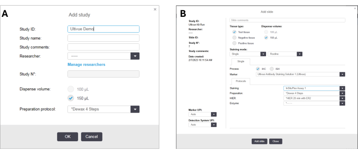
Figure 2: Prompts for the software. (A) New study prompt on Autostainer software, showing correct settings for multiplexed immunofluorescence (mIF) staining protocol. (B) Add Slide prompt on the software, showing the correct settings for mIF staining protocol. Please click here to view a larger version of this figure.

6. Imaging

1. After the staining protocol is complete, remove stained slides and coverslip in the mounting medium. Allow the mounting medium to cure in the dark until the coverslip is firmly affixed in place (typically 1 h or more, pause point).
2. Image slides on a fluorescence microscope or whole-slide scanner with appropriate filters for the assay. The dyes used in this assay are typically compatible with filters for DAPI, FITC, TRITC, Cy5, and Cy7.
3. Images will appear similar to those in Figure 3A. Visually ensure that all areas of the tissue are properly in focus and that signals appear at an appropriate intensity level (not over/underexposed). If necessary, re-image slides with different exposure settings.
4. After imaging, if an additional round of imaging is necessary, soak the slides in 1x PBS until the coverslips fall off by themselves. (pause point)

7. Exchange protocol initial set up

1. If the software is version 7.0 or later, there will be a pre-installed template of the autostainer protocol. At the bottom of the screen check that the Preferred Status selection is set to All. The template protocol will be named *ISP Signal Exchg. For earlier versions of software, the protocol can be found in Table 3.
2. Right-click on *ISP Signal Exchg and copy the protocol. In the resulting pop-up window, rename the protocol Exchange Protocol 1 with the abbreviated name ISPEXCH1. Ensure that the Preferred box is checked before proceeding and assign the same kit name as established in Step 2.6.

Table 3: Protocol for multiplex immunofluorescence signal exchange protocol. Wash Buffer corresponds to BOND Wash solution. All other ancillary reagents have correspondingly named kit components. This protocol is compatible with software version 7.0 and above, BXD 39 and above. Please click here to download this Table.

8. Exchange protocol setup and running

1. Thaw the exchange buffer at room temperature. Keep the exchange neutralizer and exchange initiator at -20 °C until use. Two reagent titration containers and the detection kit are needed to perform the exchange protocol.
2. Prepare the exchange solution in the corresponding container. The required volume is 350 + (450 µL x number of slides), and it is comprised of an exchange initiator diluted 1:500 in the exchange buffer. Do not vortex the exchange enzyme or completed exchange solution, mix by pipetting only.
3. Prepare the second fluorescent probes mix in the fluorescent probes 2 container. The required volume is 350 + (450 µL x number of slides) and is comprised of the fluorescent probes 2 solution diluted 1:20 and the exchange neutralizer diluted 1:40 within probe buffer 2. The fluorescent probe mix and probe buffer may be vortexed, but the exchange neutralizer and final combined solution should only be pipette mixed.
4. Once all reagents are prepared, place the full wand onto the autostainer and allow the reagents to be dip-tested by the machine.
5. Add all slides following step 5. During slide addition, change the marker to *Negative. For Preparation, HIER, and Enzyme, select the *---- option, as no dewax or antigen retrieval is needed for the exchange protocol. Once this is complete, click Add Slide.
6. Repeat this process as needed for the number of slides to be run in the study, ensuring that the Slide Comments field is updated for each slide added so they can be uniquely identified later.
7. After all slides are added, close the Add Slide window and print all labels, affixing them to their corresponding tissue sections.
8. Load each slide onto the tray and place cover tiles on top of each section before loading the tray onto the software.
9. Once all reagents and slides are added, select the Corresponding Autostainer in the software; this will be on the right-hand side. Once this is selected, all three slide trays and information for all reagents on the software will be visible, including bulk reagents and those added during reagent preparation.
10. Ensure that the bulk reagent containers are filled and the waste containers have enough volume remaining to complete the run.
11. After this is confirmed, press the Play button to begin the run. The protocol takes approximately 90 min to complete. Make note of the stop time and ensure the slides are removed promptly once the run is complete.

9. Imaging

1. Repeat imaging for the new round of probes, as in step 5. Images will appear as in Figure 3B.

10. Stacking (for >4-plex protein imaging)

1. Multiple images will now exist for the same slide. Combine the images in the image co-registration software to generate a stacked 8-plex image.
2. Co-register the images of each round as follows.
   1. Each round image is named as follows: _ where is the unique name of the slide (barcode) and is a string that, when sorted alphabetically, will put the round 1 image first, the round 2 image second. E.g., for = 1234ABC, files may be named 1234ABC_Round1 and 1234ABC_Round2, with all files having the appropriate extension (e.g., .czi) of the scanner. Put all of the round images in a single folder called e.g., Source Images.
   2. Within the co-registration software, click the Set button in the source images directory section of the user interface and when asked, select the Folder Created Above.
   3. Set the file type in the Source images section to the extension of the source images (e.g., .czi, .qptiff, etc.). The software will now display the two round images together in a table showing that Slide 1234ABC has 2 round images.
   4. If desired, set the location of the output stacked images to a different directory than the source images folder using the Set button in the stacked images directory section of the user interface and when asked, choose the Desired Output folder. Otherwise, the source images folder will be used by default.
   5. By default, only a .afi file representation of the stack is created. Check the option to save an OME.tif file of the entire stack in the processing options section of the interface.
   6. In order to validate the co-registration accuracy over the entire sample, check the Validation option in the output section of the interface.
   7. Press the START button to start image co-registration.

11. Image analysis

1. After slides are imaged, visualize and analyze the slides using any analysis method of choice, such as Ultivue's STARVUE image processing suite or QuPath¹⁵.

Results

Following the protocol above, FFPE tissue will be stained with multiple targets, and high-quality images of all of the markers in groups of four have been obtained (Figure 3A,B). The image co-registration software will allow images from the same slide to be combined and co-registered, as seen in Figure 3C. Similar results are shown in Figure 4 for a colorectal cancer (CRC) tissue slide.

Protocol success should be determined by assessing the expected staining pattern. In the CRC example shown, each of the stained targets is expressed in the expected subcellular compartment e.g., nuclear FoxP3, membranous CD3, cytoplasmic CD68 (Figure 4B-D). Each of the functional targets is expressed on the appropriate cell type, as demonstrated by the example of co-localization of PD1 and CD3 or of PDL-1 and CD68, which show exhausted T cells and immune-suppressive macrophages, respectively. Assessment of good signal-to-background ratio, allowing successful distinction of true positive signal from potential background noise, is usually qualitatively performed by pathologists or image analysis experts that confirm the quality of the staining, allowing successful image analysis. To further confirm staining quality and performance, comparison to the gold standard IHC (chromogenic DAB) on serial sections can be added (see example in Figure 5), as well as a positive control tissue sample such as human tonsil which for most immune targets, can be useful to confirm the success of the staining run. Note that cancers may show lower expression of targets than human tonsil¹⁶.

After the results are confirmed qualitatively, quantitative analysis can be carried out. In this work, this consists primarily of calculating the cell density of different phenotypes (number of cells/mm²) expressing a certain target or targets, as well as calculating the average intensity levels of functional targets that can show a broad dynamic range of expression. When assessing the precision of mIF assays, serial sections stained with the same markers should show comparable signals between slides, which can be seen qualitatively in Figure 6. Example quantitative results of single marker densities in different tissue types are shown in Figure 7. Image analysis on these images enables positive cells to be identified, and a corresponding positive cell density can be calculated for each marker, as well as the average signal intensity per positive cell. This allows a coefficient of variability (CV) to be calculated for each marker to assess the precision of the multiplexing assay (Table 4).

Figure 3: Images of a tissue microarray (TMA) core obtained from successive rounds of staining in 8-plex immunofluorescence protocol. (A) Image obtained from the first round of imaging, featuring markers CD8, PD1, PD-L1, and CD68. After the exchange protocol, (B) shows the second round of imaging on the same slide for the second round of markers CD3, CD4, FoxP3, and CK/SOX10, and (C) shows a co-registered image combining images (A) and (B). Please click here to view a larger version of this figure.

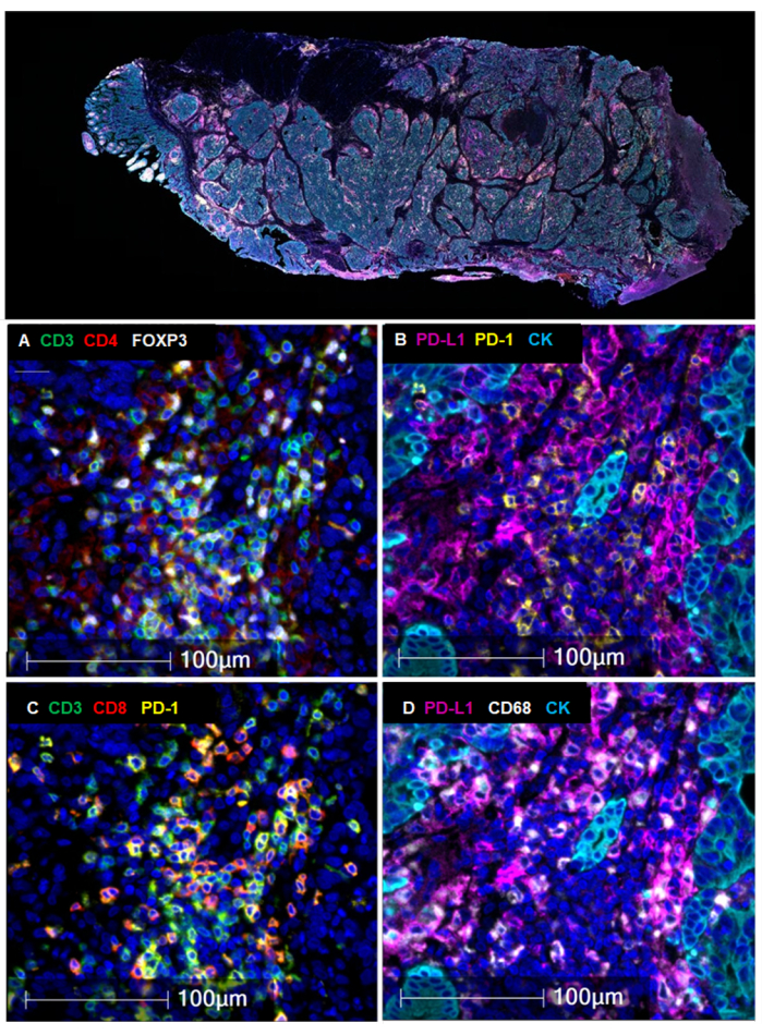
Figure 4: Representative staining of colorectal cancer (CRC) tissue with 8-plex immunofluorescence staining. The figure shows cellular phenotypes that can be identified by co-localizing multiple targets in the same cell. (top) Whole-slide image of CRC tissue. (bottom) Detailed views of regions of tissue highlighting (A) T-reg cells (CD3+/CD4+/FOXP3+), (B) PD-1- and PD-L1-expressing cells within tumor and stroma, (C) exhausted cytotoxic T cells (CD3+/CD8+/PD-1), (D) immune evading tumor cells (PD-L1+/CK+) and immune-suppressive macrophages (CD68+/PDL1+). Please click here to view a larger version of this figure.

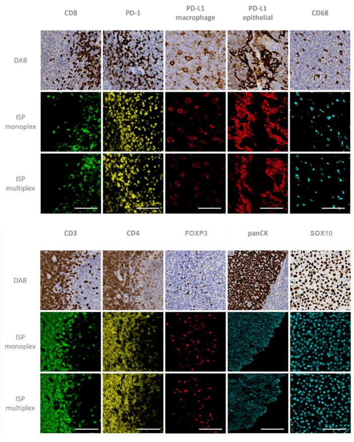
Figure 5: Qualitative comparison of immunohistochemistry (IHC) to immunofluorescence (IF) staining. Serial sections stained with single-marker immunohistochemistry stain (DAB, top row), single-marker immunofluorescence (ISP monoplex), and single-channel view of multiplex immunofluorescence (ISP multiplex) demonstrating qualitative concordance between the different staining methods. Scale bars = 100 µm. Please click here to view a larger version of this figure.

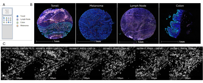
Figure 6: Serial section staining. (A) Diagram showing the layout of a multi-tissue TMA. (B) Representative 8-plex images of tissue cores of each tissue type in the TMA. (C) Representative images of CD8 in a tonsil core across six serial TMA sections stained in a single run. Please click here to view a larger version of this figure.

Figure 7: Single-marker density quantification per tissue type included in the TMA. Densities per tissue are the average densities across three representative cores of each tissue type on the TMA slide. The y-axis represents the single marker densities in different tissue types on the x-axis, in units of positive cells/mm². Please click here to view a larger version of this figure.

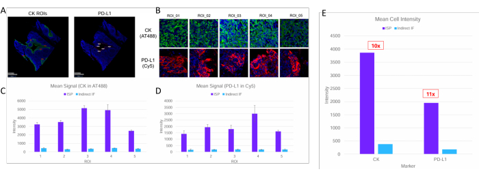
Figure 8: Region of interest (ROI) analysis of relative fluorescent signal comparing the amplified ISP mIF described in this protocol to indirect IF. (A) Representative slide stained for CK (left) or PD-L1 (right) with five ROIs indicated. (B) Representative ROI images for CK (top) and PD-L1 (bottom). Mean signal intensity achieved with amplified mIF (purple) and indirect IF (blue) for (C) CK and (D) PD-L1 across five ROIs, each measuring 100 µm x 100 µm and containing approximately 200 cells. Y-axis values show arbitrary fluorescent units and error bars show standard deviations (n=3). (E) Relative signal intensity achieved with amplified ISP mIF (purple) and indirect IF (blue) was calculated by taking the ratio of the mean amplified mIF signal to the mean indirect IF signal across all ROIs. Please click here to view a larger version of this figure.

Table 4: Calculated coefficient of variance (CV). The CV of positive cell density and mean signal intensity for the tonsil images are shown in Figure 6. Please click here to download this Table.

Discussion

This report describes a protocol for high-throughput, high-sensitivity multiplex immunofluorescence staining run using an autostainer. When conducting this protocol, the reagent preparation steps are critical and deserve attention. It is necessary to ensure reagents are mixed appropriately and correctly measured out to minimize staining variability between different slides in the same run or between different runs using the same components.

Common issues when carrying out this protocol include not mixing reagents properly prior to loading and the potential for tissue loss due to an improper de-coverslipping procedure. While this staining protocol is applicable to any FFPE tissue type, including cancer types, some tissue types may require more careful handling (e.g., tissues with high-fat content). To avoid tissue loss, allow the cover slipped slides to soak for a sufficiently long time that the coverslip detaches by itself. Do not force the coverslip to dislodge or pry the glass off.

A limitation is that while many of the most commonly used targets in immune-oncology are validated and ready to use, some targets may require assay development before being included in a multiplex panel. While this process is relatively fast, this could necessitate an additional few weeks before being able to use a custom multiplex panel.

There are several differences between this assay and other multiplex immunofluorescence technologies. Compared to direct and indirect immunofluorescence-based technologies, the assay demonstrated here has a significantly higher level of amplification, allowing for significantly improved signal-to-noise, particularly in channels that tend to show tissue autofluorescence, such as the FITC channel. This results in a ~30x stronger signal than direct immunofluorescence and ~10x stronger signal than indirect immunofluorescence as quantified by using whole-slide intensity analysis and manual ROI-based analysis (Figure 8). This method enables much more sensitive target protein detection at substantially lower exposure times and eliminates the need for image manipulation, including background subtraction that runs the risk of removing low-intensity signals.

Compared to mIF assays based on enzyme-catalyzed amplification, the assay demonstrated here has a significantly improved ability to carry out multiplexing, in addition to having a simpler workflow and generally shorter assay run time (Figure 1). In this assay, antibodies are added together in a single step and amplified simultaneously, greatly simplifying the assay protocol. Furthermore, some enzyme-based technologies, such as tyramide signal amplification (TSA), can show interference between different antibodies, in what is termed the umbrella effect^12,17,18. The amplification technology used here avoids this problem, allowing the detection of multiple colocalized and co-expressed markers on the same cell, as can be seen in Figure 4.

Approximately 90% of human cancers rise from epithelial cells¹⁹. This is because they often form the first line of defense against the external environment and proliferate faster, leading to faster accumulation of potentially oncogenic mutations. Here, inflammation plays a critical role in tumorigenesis, progression, and dissemination. Over the past decade, many therapies targeting immune checkpoint inhibitors and immune cells have emerged as a powerful arsenal against many tumor types^5,20,21. However, a significant portion of the patients still do not respond. It is likely that the tumor microenvironment (TME) and the local immune landscape play a critical role. By profiling TME molecular signatures associated with differential drug response across many patients, it might be possible to better define therapeutic biomarkers. This report demonstrates that mIF technology can be used to profile multiple protein biomarkers in parallel, including markers with low expression, across hundreds of whole sample slides or tumor microarrays.

Materials

List of materials used in this article

Name	Company	Catalog Number	Comments
Anti-CD3	Ultivue		Clone BC33 (BioCare). Part of ULT50801
Anti-CD4	Ultivue		Clone SP35 (Abcam). Part of ULT50801
Anti-CD68	Ultivue		Clone KP1 (BioCare). Part of ULT50801
Anti-CD8	Ultivue		Clone C8/144B (BioCare). Part of ULT50801
Anti-Cytokeratin + Anti-SOX10	Ultivue		Clones AE1/AE3 (Bethyl Labs) and BC34 (BioCare). Part of ULT50801, provided as a mixture
Anti-FOXP3	Ultivue		Clone 236A/E7 (Thermo). Part of ULT50801
Anti-PD1	Ultivue		Clone CAL20 (Abcam). Part of ULT50801
Anti-PDL1	Ultivue		Clone 73-10 (Abcam). Part of ULT50801
Axioscan.Z1 Microscope	Zeiss		called fluorescence microscope in text
Bond Dewax Solution	Leica	AR9222
Bond Epitope Retrieval Solution 2	Leica	AR9640
Bond Open Containers, 30 mL	Leica	OP309700
Bond Research Detection Kit	Leica	DS9455
Bond Titration Inserts	Leica	OPT9049
Bond Titration Kit	Leica	OPT9719
Bond Universal Covertiles	Leica	S21.4611
Bond Wash Solution 10x Concentrate	Leica	AR9590
BondRX Autostainer	Leica		called "autostainer" in text
BondRX Software	Leica		Version 6.0 or later
Coverslips, #1.5 thickness	Corning	2980-244
Ethanol, 200 proof	VWR	89370-084
FFPE tissue blocks	BioIVT		tissue types vary
OmniVUE 8-plex assay (CD3, CD4, CD8, CD68, FOXP3, PD-1, PD-L1, pan-Cytokeratin/SOX10)	Ultivue	ULT50801	contains all other Ultivue components
Phosphate-buffered saline (PBS)	Boston BioProducts	C-9911F	(pH 7.4 with 2.7 mM KCl and 137 mM NaCl)
ProLong Gold Antifade Mountant	Thermo	P10144	called "mounting medium" in text
UltiAnalyzer.AI	Ultivue
UltiStacker.AI	Ultivue
Ultivue Amplification Buffer	Ultivue		part of ULT50801
Ultivue Antibody Diluent	Ultivue		part of ULT50801
Ultivue Exchange Buffer	Ultivue		part of ULT50801
Ultivue Exchange Initiator	Ultivue		part of ULT50801
Ultivue Exchange Neutralizer	Ultivue		part of ULT50801
Ultivue Fluorescent Probes 1	Ultivue		part of ULT50801
Ultivue Fluorescent Probes 2	Ultivue		part of ULT50801
Ultivue Pre-Amplification Mix	Ultivue		part of ULT50801
Ultivue Probe Buffer	Ultivue		part of ULT50801
Ultrapure water	Sigma-Aldrich	W4502

References

- McGinnis, L. M., Ibarra-Lopez, V., Rost, S., Ziai, J. Clinical and research applications of multiplexed immunohistochemistry and in situ hybridization. J Pathol. 254 (4), 405-417 (2021).
- Tan, W. C. C., et al. Overview of multiplex immunohistochemistry/immunofluorescence techniques in the era of cancer immunotherapy. Cancer Comm. 40 (4), 135-153 (2020).
- Huss, R., Schmid, C., Manesse, M., Thagaard, J., Maerkl, B. Immunological tumor heterogeneity and diagnostic profiling for advanced and immune therapies. Adv Cell Gene Ther. 4 (3), e113(2021).
- Singhal, S. K., et al. Kaiso (ZBTB33) subcellular partitioning functionally links LC3A/B, the tumor microenvironment, and breast cancer survival. Comm Biol. 4 (1), 1-13 (2021).
- Patil, N. S., et al. Intratumoral plasma cells predict outcomes to PD-L1 blockade in non-small cell lung cancer. Cancer Cell. 40 (3), 289-300.e4 (2022).
- Hong, D. S., et al. Autologous T cell therapy for MAGE-A4+ solid cancers in HLA-A*02+ patients: a phase 1 trial. Nat Med. 29 (1), 104-114 (2023).
- Robbins, C. J., et al. Multi-institutional Assessment of Pathologist Scoring HER2 Immunohistochemistry. Mod Pathol. 36 (1), 100032(2023).
- Ko, H., et al. Is HER2-Low a New Clinical Entity or Merely a Biomarker for an Antibody Drug Conjugate. Oncol Ther. 12 (1), 13-17 (2024).
- Fundytus, A., Booth, C. M., Tannock, I. F. How low can you go? PD-L1 expression as a biomarker in trials of cancer immunotherapy. Ann Oncol. 32 (7), 833-836 (2021).
- Im, K., Mareninov, S., Diaz, M. F. P., Yong, W. H. An Introduction to Performing Immunofluorescence Staining. Method Mol Biol. 1897, 299-311 (2019).
- Sheng, W., et al. Multiplex Immunofluorescence: A Powerful Tool in Cancer Immunotherapy. Int Mol Sci. 24 (4), 3086(2023).
- Taube, J. M., et al. The Society for Immunotherapy of Cancer statement on best practices for multiplex immunohistochemistry (IHC) and immunofluorescence (IF) staining and validation. J ImmunoTher Cancer. 8 (1), e000155(2020).
- Myers, J. A review of automated slide stainers for immunohistochemistry and in situ hybridization. Medl Lab Obser. 40 (1), 41-44 (2008).
- Schwarze, J. K., et al. Intratumoral administration of CD1c (BDCA-1)+ and CD141 (BDCA-3)+ myeloid dendritic cells in combination with talimogene laherparepvec in immune checkpoint blockade refractory advanced melanoma patients: a phase I clinical trial. J ImmunoTher Cancer. 10 (9), e005141(2022).
- Bankhead, P., et al. QuPath: Open source software for digital pathology image analysis. Sci Rep. 7 (1), 16878(2017).
- Koppel, C., et al. Optimization and validation of PD-L1 immunohistochemistry staining protocols using the antibody clone 28-8 on different staining platforms. Mod Pathol. 31 (11), 1630-1644 (2018).
- Parra, E. R., et al. Procedural Requirements and Recommendations for Multiplex Immunofluorescence Tyramide Signal Amplification Assays to Support Translational Oncology Studies. Cancers. 12 (2), 255(2020).
- Surace, M., et al. Automated Multiplex Immunofluorescence Panel for Immuno-oncology Studies on Formalin-fixed Carcinoma Tissue Specimens. J Vis Exp. (143), e58390(2019).
- Hinck, L., Näthke, I. Changes in cell and tissue organization in cancer of the breast and colon. Curr Opin Cell Biol. 0, 87-95 (2014).
- Alturki, N. A. Review of the Immune Checkpoint Inhibitors in the Context of Cancer Treatment. J Clin Med. 12 (13), 4301(2023).
- Sun, Q., et al. Immune checkpoint therapy for solid tumours: clinical dilemmas and future trends. Signal Transduct Targeted Ther. 8 (1), 1-26 (2023).
Reprints and Permissions