Comprehensive Analysis of Drug Response using the FLICK Assay

Summary

This protocol describes how to use the FLICK assay for evaluating drug responses, including detailed instructions for using this assay to compute the drug-induced growth rates and death rates and to evaluate the mechanism of drug-induced cell death.

Abstract

For understanding drug efficacy, a critical need is to characterize the extent of drug-induced cell death. Efforts to quantify the level of drug-induced cell death are challenged by the existence of more than a dozen molecularly distinct forms of regulated death, each with its own activation timing and biochemical hallmark features. Furthermore, for some necrotic death subtypes, hallmark features are only observed transiently and are rapidly lost due to cell rupture. Thus, even when using a combination of death pathway-specific assays, it is challenging to accurately quantify the total amount of cell death or the relative contributions of each death subtype. Another issue is that many death-specific assays ignore how drugs affect cell proliferation, making it challenging to interpret if a drug-treated population is expanding or shrinking. The FLICK assay allows for quantification of the total level of cell death following stimulation in a manner that is specific to death but also largely agnostic to the type(s) of death activated. Additionally, the FLICK assay retains information about the total population size and cell proliferation rate. In this manuscript, we describe the basic use of the FLICK assay, how to troubleshoot this assay when using different types of biological material, and how to use the FLICK assay to quantify the contributions of each type of cell death to an observed drug response.

Introduction

For anti-cancer drugs, pre-clinical evaluation of drug sensitivity generally involves testing how drugs affect the viability of cells in culture¹. Cell viability following drug exposure is a product of at least two separate effects: drug-induced inhibition of cell proliferation and activation of cell death². Unfortunately, although cell death is a critical feature that is required for durable drug responses, standard approaches fail to clarify the degree to which a drug activates cell death³.

Common drug response assays include those that directly count cells (e.g., Coulter Counter, some uses of flow cytometry or microscopy), quantify the ability of cells to proliferate (e.g., colony formation assay), or quantify a metabolic activity (e.g., CellTiter-Glo, tetrazolium based MTT or MTS assays). A shared feature of these assays is that the data generated is proportional to the number of live cells. Because drugs vary considerably in how they coordinate growth inhibition and cell death, the number of live cells following drug exposure provides an unreliable insight into the level of drug-induced cell death³. Furthermore, because cancer cells generally proliferate rapidly in cell culture, the number of live cells can be dramatically reduced relative to the untreated population without inducing any cell death⁴. Thus, a central flaw is that the degree of cell death cannot be quantified without measuring both the number of live and dead cells.

Quantifying the number of dead cells following drug exposure is challenging to do accurately for several reasons². First, more than a dozen regulated cell death pathways exist^5,6,7,8. Although biochemical markers generally exist for identifying each type of regulated cell death, these markers vary in their specificity, and no single assay can be used to simultaneously quantify all death subtypes. Secondly, the timing of activation for each form of cell death can vary quite dramatically depending on the context, so a complete picture cannot emerge unless death is quantified over time^9,10. Many biochemical assays for quantifying cell death produce an end-point measurement, so generating kinetic data can be challenging and limited by cost. A third complication is that the dead cell itself is a transient intermediate state between the live cell state and dissociated cell debris. The stability of dead cells varies depending on the death subtype, with some types, such as apoptosis, creating relatively stable corpses, whereas other types of death cause rapid lysis. Thus, methods of quantifying death that require collection and counting of dead cells also will produce a biased understanding of cell death. Finally, a fourth limitation is that biochemical assays that quantify the degree of cell death typically fail to provide any insight into how a drug alters proliferation. Thus, the overall population size - and, importantly, whether the population is expanding or shrinking - cannot be interpreted.

Some microscopy-based assays, such as STACK and SPARKL, are effective at measuring live and dead cells over time, and these assays can produce comprehensive insights about drug-induced cell death^10,11. These assays, however, require specialized instruments, such as the Incucyte microscope, creating limitations in throughput and access to these approaches. Additionally, microscopy-based techniques require that dead cells remain in the focal plane of the microscope throughout the duration of the experiment, compromising the ability to quantify dead cells when they lose adherence from the plate or over time as dead cells decay. Similarly, microscopy-based assays face challenges when applied in the context of suspension cultures, as cells drift in and out of a given focal plane.

To address the issues highlighted above, we have generated an assay called FLICK (Fluorescence-based and Lysis-dependent Inference of Cell Death Kinetics)^12,13. The goal of the FLICK assay is to determine the level of drug-induced cell death, regardless of how the cells are dying. The FLICK method uses cell impermeant dyes, whose fluorescence depends on DNA binding. A key feature of FLICK is the use of these fluorophores to label dead cell accumulation over time by virtue of their accessible DNA, followed by a mechanical detergent-based lysis to permeabilize any live cells at the end of the assay. These data, combined with mathematical modeling, enable the quantification of both live and dead cell populations with continuous temporal resolution and without requiring the collection or handling of dead cells. Furthermore, the use of a plate reader to evaluate dead cell fluorescence allows for the evaluation of dead cells without requiring that dead cells remain intact, thus alleviating a bias against necrotic forms of death that result in cell rupture. Finally, the FLICK assay requires minimal plate handling and can rapidly generate kinetic measurements, allowing for high-throughput drug screening. In this protocol, we focus on the use of the FLICK assay, including how to use FLICK to infer the drug-induced growth rate, death rate, and/or the mechanisms of cell death.

Protocol

1. Optimization of permeabilization time for each cell line of interest

NOTE: The volumes and amounts described are for optimizing one cell line. These values should be scaled up based on the number of cell lines that are to be tested.

1. Plate the desired number of cells in each well of a 96-well, optical bottom, black-walled plate. Add 100 µL of complete medium and let the cells adhere to the plate overnight.
   NOTE: The plated cell number should be optimized with consideration for the growth rate of the cells, optimal densities, and length of the assay. Typical starting cell numbers for adherent cancer cell lines measured over 72 h are 1500 - 5000 cells per well. For instance, U2OS cells may be plated at 2000 cells per well in DMEM with 10% FBS, 2 mM glutamine, and 1% Pen-Strep and cultured overnight in standard conditions (5% CO₂, 37 °C, with humidity).
2. In a 15 mL conical centrifuge tube, prepare 1.5 mL of a 1.5% solution of Triton-X in phosphate buffered saline (PBS). Vortex the 1.5% Triton-X solution for 5 s at max speed. Place in a 37 °C water bath for at least 30 min.
3. Visually inspect the solution to ensure that Triton-X has fully dissolved by vortexing for several seconds. Ensure that the solution is homogenous.
4. Add 10 µL of the 1.5% Triton-X solution to each well of the plated cells. Do not mix.
   NOTE: At this stage, it is not desirable to mix using repeated pipetting due to the formation of bubbles.
5. Return cells to the 5% CO₂, 37 °C with humidity cell culture incubator for at least 1 h.
   NOTE: Following application of the Triton-X solution, most cell lines are fully lysed in 2-3 h. Waiting up to 24 h has minimal impact on fluorescence signal when using dyes such as SYTOX Green. Increasing the percentage of Triton-X may shorten incubation time for difficult to lyse cell lines.
6. Observe cell morphologies on a light microscope using a 10x objective. Inspect cells once every hour until cell bodies are no longer visible. Record the time required for cell permeabilization.
   NOTE: If a fluorescent microscope is available, lysis can be visualized using a cell-impermeable DNA dye, such as SYTOX Green. The dye can be added at a 10x final concentration to the Triton-X solution, and permeabilization can be confirmed by fluorescence microscopy.

2. Selection and calibration of DNA stain

NOTE: A requirement for the FLICK assay is the use of a cell impermeant fluorophore that emits a signal in a DNA-binding dependent manner, does not affect cell viability, and produces a signal that scales linearly with cell number. This protocol uses SYTOX Green. Other dyes with similar properties may also be suitable for the FLICK assay, but these should each be evaluated and calibrated. See Table 1 for examples.

1. For the selected DNA dye, determine the range of concentrations to be tested based on the manufacturer's recommendation.
2. For each concentration to be tested, plate 40,000 cells in 180 µL of cell culture medium in triplicate along the leftmost column of a 96-well, optical bottom, black-walled plate. Add 90 µL of medium to the remaining wells.
   NOTE: This will be used to generate a linear cell titration across the rows of the plate. The final concentration of the first wells will be 20,000 cells/well. Optical bottom plates are not required for plate readers that read fluorescence from the top of the well. The cell culture medium should be the same medium used for growing the cells being tested. For instance, if using U2OS cells, 40,000 cells should be resuspended in 180 µL of DMEM.
3. Using a multichannel pipette, create a 1:2 serial dilution by transferring 90 µL from the leftmost column into the adjacent column to the right. Pipette 15x to mix.
4. Repeat step 2.3, moving from the second column to the third column, then from the third column to the fourth column, and so on. Finish the titration in the second to last column of the plate. Leave the last column without cells so the background signal of cell culture media can be obtained.
5. For the second-to-last column, remove 90 µL so all wells have 90 µL of medium containing a varied number of cells. Let cells adhere for 6 h in a 37 °C cell culture incubator.
6. Prepare a 10x solution of DNA dye for each concentration of dye to be tested, with the DNA dye diluted into complete growth media used for culturing the cells of interest. Prepare 1.5 mL of a 1.5% Triton-X solution in PBS, as described in step 1.
7. To each well of the 96-well plate, add 10 µL of the 10x DNA dye. Add 10 µL of 1.5% Triton-X solution to each well to permeabilize cells. Incubate cells in this solution for the optimal time, which was determined in step 1.
   NOTE: After the addition of Triton-X, the final concentration of DNA dye is slightly less than 1x, but this is inconsequential. Following incubation, the entire plate should be lysed. The manual cell titration will be used to identify the optimal DNA dye concentration and the optimal settings for acquiring fluorescence.
8. Measure fluorescence intensities across the cell titration plate. Quantify fluorescence over a range of acquisition settings as outlined by the manufacturer of the DNA dye. Depending on the plate reader used, modify the excitation and emission wavelengths and/or the digital gain.
9. Remove the background signal from each measurement by subtracting the average signal of the column containing no cells. These values can be found in the right-most column of wells in the serial dilution plate.
10. Determine the linearity of each concentration of DNA dye for each acquisition setting. Linearity can be determined by graphing the cell number against the fluorescence signal and performing linear regression. The coefficient of determination (r²) reports the degree to which the fluorescence signal is linearly related to the cell number.
11. Pick the acquisition settings and DNA dye concentration that has the best combination of linearity and dynamic range.
    NOTE: Consider the entire range of cell numbers from 0 to 20,000 cells. Ensure that the gain and DNA dye concentration are linear at low cell numbers, between 0 and 1000 cells. Several instrument settings or DNA dye concentrations may provide a strong correlation over the whole range. However, it is essential that the low-end sensitivity is robust, such that small changes in dead cells can be accurately measured.

3. Cell Plating, In-Well Drug Application, and Dead Cell Fluorescence Measurement Over Time in Drug-Treated Plates

NOTE: Drug dilution plates can be designed flexibly based on experimental needs. Generally, drug dilution plates will include a log or semi-log dilution series of one or several drugs.

1. Consider the optimal plating layout for the experiment. Avoid measurements from the outer wells of a 96-well plate to decrease noise associated with growth variation, as the outer wells experience different temperatures, oxygenation, and evaporation compared to the inner wells of the plate.
   NOTE: Including controls throughout the landscape of the plate will increase the robustness of the growth data. Consider including control wells in the center and edges of the plate.
2. Determine the number of plates required for the experiment. Include one additional plate to be lysed at the beginning of the assay to establish the average cell number per well at the time of drugging (i.e., the T0 control plate).
3. Prepare a cell suspension in complete growth media.
   1. Based on the number of plates needed for the experiment (calculated in step 3.2), determine the volume of the cell suspension required. If seeding plates at 90 µL per well, about 10 mL is required per plate. Multiply the number of plates required by 10 mL.
      NOTE: It is desirable to increase this volume to account for the dead volume of the reservoir and volume loss during pipetting. For instance, the calculated volume may be multiplied by 1.2.
   2. Count cells and prepare a cell dilution based on the desired number of cells per well. For instance, if aiming to seed 2000 cells in 90 µL of media per well of a 96-well plate, for 3 total plates, calculate the total number of cells needed for the experiment as below:
      
      Similarly, if the counted cell suspension is 400,000 cells/mL, the volume of the cell suspension needed for the experiment would be:
      
   3. Correct the volume of cell culture media used for plating by subtracting the volume of the counted cell suspension to be added.
      36 mL media - 2 mL cell suspension = 34 mL corrected media volume
4. Mix the counted cell suspension with the correct media volume using a serological pipette. Transfer this cell suspension to a V-bottom reagent reservoir.
5. Using a multichannel pipette, add 90 µL of the cell suspension to each well of the 96-well plates. Mix the cell suspension in the reagent reservoir regularly using repeated pipetting with a serological pipette to ensure that the desired to ensure that the desired concentration of cells per volume is maintained.
6. Let cells adhere overnight in a 37 °C cell culture incubator (generally 12-24 h).
7. Prepare a 1.5% Triton-X solution in PBS, as described in step 1. The volume of this solution should be sufficient to lyse all plates. About 1.5 mL of 1.5% Triton-X in PBS is sufficient to lyse one 96-well plate.
   NOTE: The 1.5% Triton-X solution in PBS is stable for over a week and can be made in advance for convenience.
8. Determine the amount of cell culture media required for making a drug dilution plate. Prepare drug dilution plates in U- or V-bottom 96-well clear plates.
   1. To ensure that the volume of diluted drug is sufficient for the experiment, increase the minimum required volume to account for volume loss during pipetting. For example, if drugs are to be added in 10 µL to each well of a 96-well plate and the experiment includes three plates, 30 µL of diluted drug are required per well. Prepare 40-50 µL of drugged media per well to account for volume loss. Add 1.5 mL to the volume of media required to account for the media needed for the T0 control plate.
9. Prepare a 10x concentration of the selected DNA dye in complete growth media. This concentration is based on the concentration selected in step 2.11. The total volume of this solution is calculated in step 3.8.
10. Using the DNA dye + growth medium from step 3.9, prepare a 10x concentration of each drug to be tested. Create only the highest dose of each drug in the drug dilution plate and serially dilute the drugs with a multichannel pipette, mixing 15x between each well.
    NOTE: When making the highest dose for a given drug in the drug dilution plate, the volume of the drug should be accounted for to ensure that the concentration is accurate.
11. Using a multichannel pipette, add 10 µL of drug + DNA dye solution from step 3.10 to the plates containing cells.
    NOTE: For drug dilution plates in which a serial dilution was created, if drugs are added to the cells starting with the lowest concentration of drug and working up to the highest concentration, the tips of the multichannel pipette do not need to be changed. However, tips on the multichannel pipette should be changed between each plate and whenever the tips were used in a well containing a different drug or a higher concentration of the drug.
12. Read the fluorescence for all plates in which drugs were added. This fluorescence reading is the T0 reading (i.e., dead cells at Time = 0 h).
13. Return plates to the incubator after taking the T0 fluorescence reading.
14. Add 10 µL of the 10x DNA dye solution created in step 3.9 and 10 µL of the 1.5% Triton-X solution in step 3.7 to the T0 control plate. Return this plate to the incubator for the amount of time selected in step 1.8.
15. Read the T0 control plate once the cells are fully lysed, as described in step 1.6.

4. Measure the dead cell fluorescence over time for drug-treated plates

NOTE: Minimize the time plates are out of the incubator. Prolonged changes in temperature can affect cell viability, and exposure to light can compromise DNA fluorophores, such as SYTOX Green.

1. Acquire fluorescence readings for all drug-treated plates every 3-4 h after drugging. Plates do not need to be read overnight unless very precise death kinetics are required.
   NOTE: Time points do not need to be taken at fixed/standard intervals. In general, time points can be taken exclusively during normal working hours without causing errors in the downstream analysis of death kinetics. The kinetics can be inferred as long as some measurements are taken in the period before death onset, during the rising phase of death, and during the saturation/plateau phase.
2. At the desired final time point, acquire a fluorescence reading. Immediately afterward, add 10 µL of the 1.5% Triton-X solution prepared in step 3.7 to lyse the cells.
3. Return the plates to the incubator and allow the cells to permeabilize for the time determined in step 1.
4. Acquire fluorescence readings following permeabilization. This fluorescence value is proportional to the total number of cells (i.e., live + dead cells) for each well.

5. Calculate the lethal fraction kinetics

NOTE: Calculations described in this protocol can be analyzed in any format or software. However, using a programming environment such as MATLAB, R, or Python will allow for faster and more flexible analysis.

1. Calculate the average fluorescence values from the T0 control plate using the 50% trimmed mean. This value is proportional to the total number of cells prior to drugging.
2. Using curve fitting and an exponential growth function, calculate the kinetics of population growth for all wells in the experiment. The initial population size for each well is the average T0 fluorescence value calculated in step 5.1. The final population size for each well is the post-permeabilization value calculated in step 4.4. The duration of the assay is from 0 h to the assay endpoint selected in step 4.4.
3. Using the growth parameters determined in step 5.2, calculate the number of total cells at every measured time point in the assay for every well. Determine the number of live cells at each measured time point by subtracting the dead cell measurement from the total cells calculated in step 5.2.
   NOTE: Due to small amounts of noise in the assay, occasionally, the live cell number may be a small negative number. This can be manually set to 0 since there cannot be a negative number of live cells and most likely indicates all cells in that well were dead.
4. Calculate lethal fraction (LF) for each time point by dividing the dead cell fluorescence signal by the total cell signal for each time point.
5. Fit a Lag Exponential Death (LED) equation to the lethal fraction time course data¹⁰. To avoid arbitrary kinetic parameters for doses of a drug that do not induce any significant lethality, fit to a linear model with a slope equal to 0. Determine significant levels of lethality based on the noise in the assay or the LF observed for undrugged conditions.
6. Record death onset time (DO) from the LED equation. The LED equation has four parameters: the initial LF (LFi), the LF at plateau (LFp), the initial death rate (DR), and the DO. Infer these parameters from the data using a non-linear regression (i.e., curve fitting).
7. Compute the fractional viability (FV) at the assay endpoint for each drug at each dose. Subtract the endpoint LF value from 1 or divide the number of live cells by the total cells.
   NOTE: FV can be calculated at any time point, not only at the assay endpoint. These data are used to evaluate dose pharmacology (e.g., drug IC50 or EC50).

6. Calculate the GR value

1. Determine the average number of live cells for each well at the start of the assay. Calculate this value using the post-permeabilization T0 reading calculated in step 3.15 and subtracting the T0 reading for each well, which was collected in step 3.12. In the GR equation below (step 6.3), this value is referred to as x₀.
   NOTE: Occasionally the highest dose of a drug can interfere with the fluorescence reading of the DNA dye. It may be desirable to compute the average number of live cells at time 0 using the control wells.
2. For the control wells (x_ctrl), determine the average number of live cells for each well at the assay endpoint. Determine the average number of live cells at the assay endpoint for each drug treated condition (x(c)).
   NOTE: Depending on the variation in cell growth across the plate, different x_ctrl values can be used for normalization of each well. For instance, if the x_ctrl values vary systematically across the plate, it may be desirable to use the closest x_ctrl value rather than the plate's average x_ctrl value.
3. For each drug-treated well, compute the normalized growth rate inhibition value (GR) using the following equation⁴:
   
   Perform curve fitting using a 4-parameter logistic regression. GR is on a scale from -1 to 1.

7. Calculate drug-induced growth and death rates using the GRADE method

NOTE: GR represents the net population growth rate, not the true cell proliferation rate. The drug-induced population growth and death rates can be computed using a combination of the GR and the lethal fraction (LF).

1. Determine the doubling time (τ) of the cell line during the experiment using the average number of live cells from the T0 control reading (x₀), the average number of live cells from the control condition at assay endpoint (x_ctrl), and the length of the assay in hours (t) to solve the following equation:
   
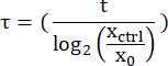
   NOTE: Accurate calculation of cell doubling time (τ) requires that cells continuously double throughout the length of the assay. For cells that experience contact inhibition, cells should be seeded at starting densities that will not become confluent during the desired assay time. For example, U2OS has an average doubling time of 24 h. Seeding 2000 cells per well in a 72 h assay is optimal for interpreting their growth rate.
2. Determine the relationship between growth/death rates and population size. To do this use a birth/death model and a simulation initialized with all plausible pairwise combinations of growth and death rates. This simulation requires the average number of live cells from the T0 control plate (x₀), the length of the assay (t), and a user- defined range of plausible proliferation rates (p), and death rates (d).
   
   
   1. To determine plausible values for growth rates, start with the untreated growth rate in cell population doublings per h (1/T) as the highest growth rate and 0 as the lowest growth rate. Divide this range into 500 equally spaced segments. A similar operation can be applied for the death rate, testing a range from 0 to 1.
      NOTE: All pairwise combinations of 500 rates can be performed using any programming environment but may be too computationally intense if using some software. Reducing this to all pairwise combinations of 50 growth and death rates can alleviate this issue, with a reduction in the precision of the inference. A spreadsheet template has been provided with this protocol.
3. Determine the GR and LF values (described above) for each simulated proliferation (p) and death (d) rate pair.
   NOTE: Steps 7.2-7.3 will generate a table that contains each theoretical pair of proliferation and death rates, with the computed GR and LF values for that theoretical pair. This will function as a look up table to associate an experimentally observed pair of GR and LF values with a pair of drug-induced proliferation and death rates. Testing more than 500 discrete values for proliferation and death rates will result in a more numerically precise value, but this level of precision will likely be beyond the precision of the assay.
4. Compute the pairwise distance between each experimentally calculated GR/LF pair and each theoretical GR/LF pair in the look up table. Infer the theoretical pair with the minimum distance to the experimentally observed pair of GR/LF values to be the true drug-induced proliferation and death rates.

8. Determination of death pathways using pathway-selective chemical inhibitors

NOTE: Chemical inhibitors alone are insufficient for definitively determining the mechanism of death for a given drug. Chemical inhibitors of death pathways should be used to determine which biochemical or phenotypic responses should be explored in subsequent experiments, which are likely to include morphological assessment, pathway-specific biochemical markers, and evaluation of genetic dependencies.

1. Optimize the dose of each cell death inhibitor in the cell line of interest by testing a dose range of inhibitor concentrations in the context of a canonical activator of the death pathway(s) of interest (Table 2). Ideally, the selected dose of inhibitor should not affect cell viability on its own (check the GR metric).
   NOTE: Not all cell lines can activate all death pathways. Biochemical or phenotypic validation may be required when testing activators/inhibitors of different death pathways.
2. Consider the optimal plating layout for an inhibitor screen. To minimize batch effects, keep each drug on the same plate as the inhibitor(s) that are being evaluated, with replicates on separate plates.
3. Seed the desired number of cells in each well of a 96-well, optical-bottom, black-walled plate, similar to step 3.3. Decrease the plating volume to 80 µL to account for the volumes of the inhibitor and drug.
4. Prepare 10x concertation of the inhibitors to be tested in complete media and add 10 µL to each well. Pre-treat cells with death pathway inhibitors for 2-4 h. Afterward, add the drugs of interest and acquire fluorescence reading, as in steps 3-5.
5. Evaluate the change in death onset time (DO) and/or the max lethal fraction to assess the effectiveness of the inhibitor(s). The DO is an inferred parameter from the Lag Exponential Death (LED) model. See steps 5.6 - 5.7.

Results

Using this protocol, we explored the sensitivity of U2OS cells to the HDAC inhibitor Belinostat. These experiments were performed using 2 µM SYTOX Green to label dead cells (Figure 1A). Kinetic readings were made using a fluorescent plate reader at a 130 gain setting (Figure 1B). Cells were lysed in 1.5% Triton-X solution in PBS for 2 h at the end of the assay (Figure 1C-D).

The FLICK pro...

Discussion

The FLICK assay is a robust method for generating a comprehensive evaluation of a drug's effect on the growth and death of a cell population. Because this method does not directly count cells, critical steps in the protocol are to ensure assay linearity and complete lysis during the triton permeabilization steps. The correct permeabilization time can be identified visually, as highlighted in this protocol, or quantitatively by reading plate fluorescence over time and identifying when the signal plateaus. In our exper...

Materials

List of materials used in this article

Name	Company	Catalog Number	Comments
Belinostat	ApexBio	A4612
Camptothecin	ApexBio	A2877
Conical centrifuge tube, 15mL	Fisher Scientific	12-565-269
DMEM	Corning	10017CV	For seeding and drugging cells
DMSO	Fisher Scientific	MT-25950CQC	For seeding and drugging cells
Fisherbrand 96-Well, Cell Culture-Treated, U-Shaped-Bottom Microplate	Fisher Scientific	FB012932	For seeding and drugging cells (pin plate)
Greiner Bio-One CELLSTAR μClear 96-well, Cell Culture-Treated, Flat-Bottom Microplate	Greiner	655090	For seeding and drugging cells
IncuCyte S3	Essen Biosciences		Any phase microscope will work
MATLAB	MathWorks	https://www.mathworks.com/products/matlab.html	MATLAB version R2023b, a license is required
Microplate fluorescence reader	Tecan	Spark	For measuring dead cell fluorescence
Palbociclib	ApexBio	A8316
PBS	Corning	21-040-CM	Any PBS works
Spark Multimode Microplate Reader	Tecan	https://www.tecan.com/spark-overview	SparkControl software version 2.2
Sterile reservoir, 25 mL	Fisher Scientific	13-681-508	For seeding and drugging cells
Sytox Green nucleic acid stain	Thermo Fisher Scientific	S7020	DNA stain for measuring dead cell fluorescence
Triton-X 100	Thermo Fisher Scientific	J66624-AP	For permeabilizing cells
U2OS	ATCC	HTB-96	An example cell line used in this protocol
Z-VAD-FMK	ApexBio	A1902

References

- Hafner, M., Niepel, M., Sorger, P. K. Alternative drug sensitivity metrics improve preclinical cancer pharmacogenomics. Nat Biotechnol. 35 (6), 500-502 (2017).
- Dixon, S. J., Lee, M. J. Quick tips for interpreting cell death experiments. Nat Cell Biol. 25 (12), 1720-1723 (2023).
- Schwartz, H. R., et al. Drug GRADE: An Integrated Analysis of Population Growth and Cell Death Reveals Drug-Specific and Cancer Subtype-Specific Response Profiles. Cell Rep. 31 (12), 107800(2020).
- Hafner, M., Niepel, M., Chung, M., Sorger, P. K. Growth rate inhibition metrics correct for confounders in measuring sensitivity to cancer drugs. Nat Methods. 13 (6), 1-11 (2016).
- Galluzzi, L., et al. Molecular mechanisms of cell death recommendations of the Nomenclature Committee on Cell Death 2018. Cell Death Differ. 25 (3), 486-541 (2018).
- Tsvetkov, P., et al. Copper induces cell death by targeting lipoylated TCA cycle proteins. Science. 375 (6586), 1254-1261 (2022).
- Holze, C., et al. Oxeiptosis, a ROS-induced caspase-independent apoptosis-like cell-death pathway. Nat Immunol. 19 (2), 130-140 (2018).
- Maltese, W. A., Overmeyer, J. H. Methuosis Nonapoptotic Cell Death Associated with Vacuolization of Macropinosome and Endosome Compartments. Am J Pathol. 184 (6), 1630-1642 (2014).
- Inde, Z., Forcina, G. C., Denton, K., Dixon, S. J. Kinetic Heterogeneity of Cancer Cell Fractional Killing. Cell Rep. 32 (1), 107845(2020).
- Forcina, G. C., Conlon, M., Wells, A., Cao, J. Y., Dixon, S. J. Systematic Quantification of Population Cell Death Kinetics in Mammalian Cells. Cell Syst. 4 (6), 1-18 (2017).
- Gelles, J. D., et al. Single-Cell and Population-Level Analyses Using Real-Time Kinetic Labeling Couples Proliferation and Cell Death Mechanisms. Dev Cell. 51 (2), 277-291.e4 (2019).
- Richards, R., et al. Drug antagonism and single-agent dominance result from differences in death kinetics. Nat Chem Biol. 16 (7), 791-800 (2020).
- Richards, R., Honeywell, M. E., Lee, M. J. FLICK: an optimized plate reader-based assay to infer cell death kinetics. STAR Protoc. 2 (1), 100327(2021).
- Honeywell, M. E., et al. Functional genomic screens with death rate analyses reveal mechanisms of drug action. Nat Chem Biol. 20 (11), 1443-1452 (2024).
- Jannoo, R., Xia, Z., Row, P. E., Kanamarlapudi, V. Targeting of the Interleukin-13 Receptor (IL-13R)α2 Expressing Prostate Cancer by a Novel Hybrid Lytic Peptide. Biomolecules. 13 (2), 356(2023).
- Gelles, J. D., Chipuk, J. E. Why not add some SPARKL to your life (and death)! Mol Cell Oncol. 7 (1), 1685841(2020).
Access restricted. Please log in or start a trial to view this content.
Reprints and Permissions