An Open-source Protocol for Deep Learning-based Segmentation of Tubular Structures in 3D Fluorescence Microscopy Images

Summary

This protocol introduces an open-source toolbox offering a complete pipeline for segmenting tubular structures in three-dimensional (3D) fluorescence microscopy images. Employing deep learning with simulation-based data augmentation, it trains U-Net and Attention U-Net models, provides qualitative and quantitative evaluations and includes user-friendly notebooks for training, inference, and visualization throughout.

Abstract

Segmenting tubular structures in dense biological tissues from 3D fluorescence microscopy images is critical to study complex tissue but remains challenging due to image complexity, variability, and quality issues. Here, we introduce an open-source, user-friendly toolbox for end-to-end segmentation of tubular structures in 3D images, accessible to researchers without formal programming training. The toolbox features interactive Jupyter notebooks implementing two simple yet efficient deep learning architectures -- 3D U-Net and 3D U-Net with attention mechanisms -- for precise 3D segmentation of tubular networks. A key innovation is our simulation-based data augmentation strategy, which enhances model performance even with minimal training data (as few as one 3D image). Employing user-provided masks, the protocol generates artificial microscopy images with varying signal-to-noise ratios and simulates realistic imaging artifacts, including uneven staining, point spread function convolution, axial intensity variations, and Poisson and Gaussian noise. The protocol systematically guides users through data augmentation, model training, qualitative and quantitative evaluation on test sets, and inference on new images. We validate the toolbox by analyzing two morphologically distinct tubular networks in mouse liver tissue -- the bile canaliculi and sinusoidal networks -- demonstrating that both architectures perform well, with the attention U-Net slightly outperforming the standard U-Net when trained with augmented data. Our comprehensive toolbox, executable on local Graphics Processing Units (GPUs), high-performance computing clusters, or cloud platforms, contributes to the democratization of advanced image analysis for a broad spectrum of researchers.

Introduction

Quantitative analysis of tubular structures in biological tissues, such as blood vessels, neuronal networks, and bile ducts in the liver, is fundamental for understanding physiological and pathological processes, including angiogenesis, tumor metastasis, and organ development^1,2,3. Three-dimensional (3D) fluorescence microscopy has emerged as a pivotal tool for imaging these complex networks, offering high spatial resolution and enabling the visualization of intricate tissue architectures in their native context^4,5,6,7. However, accurately segmenting tubular structures from dense biological tissues remains a formidable challenge due to imaging artifacts, signal variability, and the heterogeneous morphology inherent to biological specimens. Traditional segmentation methods, such as thresholding, region growing, and model-based algorithms, often require extensive manual intervention and meticulous parameter tuning, which can be both time-consuming and subjective, especially for complex 3D tissue such as liver^8,9,10,11,12. These approaches are frequently not robust to the variability inherent in biological samples and imaging conditions, limiting their generalizability across different datasets and experimental setups. Software tools like ImageJ¹³ and TiQuant⁸ have been developed to assist in tissue analysis and quantification; however, they may lack the flexibility or scalability needed for comprehensive 3D reconstructions of complex tubular networks in a fully automatic manner.

Deep learning has revolutionized biomedical image analysis by automating segmentation tasks with high accuracy and efficiency^14,15,16. Convolutional neural networks (CNNs), particularly encoder-decoder architectures like the U-Net, have demonstrated exceptional performance in various biomedical imaging applications^17,18,19. Moreover, the extension of U-Net to 3D data (3D U-Net) allows for effective processing of volumetric images, capturing spatial context in all three dimensions and improving segmentation accuracy for complex structures²⁰. Incorporating attention mechanisms into these architectures (Attention U-Net) further enhances performance by enabling the network to focus on salient features while suppressing irrelevant background noise^18,21,22. Despite their potential, implementing deep learning models for 3D segmentation poses significant challenges. Training these models typically requires substantial programming expertise, access to powerful computational resources, and large annotated datasets, which may not be readily available to all researchers. Annotating 3D images is particularly labor-intensive, often involving manual labeling of complex structures across numerous slices, which can be prohibitive for large datasets. While data augmentation techniques can alleviate the need for extensive training data by artificially increasing dataset diversity through transformations like rotation, scaling, and flipping, traditional augmentation methods may not fully capture the variability and complexity of biological images, especially those involving intricate 3D structures.

To address these limitations, we introduce an open-source, user-friendly toolbox for the end-to-end segmentation of tubular structures in 3D microscopy images. This toolbox employs interactive Jupyter notebooks and implements two robust deep learning methods -- 3D U-Net^17,20 and 3D U-Net with attention mechanisms^18,21 -- for accurate segmentation of 3D tubular structures without requiring extensive programming knowledge. A key innovation of our protocol is a simulation-based data augmentation strategy that enhances model performance even with minimal training data -- as few as one 3D image. By leveraging user-provided masks, the protocol generates artificial microscopy images with varying signal-to-noise ratios and simulates realistic imaging artifacts, including uneven staining, convolution with the point spread function (PSF) of confocal microscopes, axial intensity variations due to antibody penetration or scattering, and the presence of Poisson and Gaussian noise. This simulation-based augmentation not only increases the quantity of training data but also enriches the dataset with realistic variations, improving the model's generalizability to unseen data. The protocol systematically guides users through data augmentation, model training, qualitative and quantitative evaluation of model predictions on test sets, and inference on new images (Figure 1). We validate the utility of our toolbox by analyzing two morphologically distinct tubular networks in mouse liver tissue: the bile canaliculi and the sinusoidal networks. These networks present different structural characteristics and imaging challenges, providing a robust testbed for our methods.

While most existing studies focus on 2D image analysis, limiting the understanding of complex 3D architectures, our approach emphasizes 3D segmentation to capture the full complexity of tissue structures. By integrating well-established and powerful deep learning architectures with a user-friendly interface, our toolbox contributes to the democratization of access to state-of-the-art image analysis tools. Our pipeline can be executed on local GPUs, high-performance computing clusters, or cloud platforms like Google Colab, making advanced image analysis accessible to a broader range of researchers regardless of computational resources. This work contributes to the field by providing an accessible and comprehensive solution for 3D segmentation of tubular structures, facilitating quantitative analyses that are essential for advancing our understanding of tissue function and disease mechanisms.

Protocol

1. Installation and setup of the toolbox

1. Downloading the toolbox from GitHub
   1. Open a web browser and navigate to the toolbox's GitHub repository: https://github.com/hernanmorales-navarrete/3DMicroscopyImageSegmentation 
   2. Download it using Git clone (option A). Ensure Git is installed on the system; if not, download it from https://git-scm.com/downloads and install it. Open a terminal (Unix/Linux/macOS) or Command Prompt (Windows) and navigate to the directory where the toolbox is to be stored. Clone the repository by typing:
      git clone https://github.com/hernanmorales-navarrete/3DMicroscopyImageSegmentation.git
   3. Download it the ZIP file (option B). On the GitHub page, click the green Code button and select Download ZIP. Save the ZIP file to the preferred directory and extract the contents of the ZIP file.
2. Setting up the Conda environment
   1. Install Anaconda or Miniconda. If not already installed, download Anaconda from:
      https://www.anaconda.com/download or Miniconda from https://docs.anaconda.com/miniconda/. Follow the installation instructions for the operating system being used.
   2. Open a terminal or Command Prompt. Create a new Conda environment named img_seg_env with Python 3.10 by typing:
      conda create -n img_seg_env python=3.10
   3. Activate the Conda environment by typing:
      conda activate img_seg_env
      or activate img_seg_env for Windows
3. Install the required dependencies using requirements.txt. Be sure to be in the root directory of the toolbox. Install the required Python packages using pip by typing:
   pip install -r requirements.txt
   NOTE: This command reads the requirements.txt file and installs all necessary packages
   1. Confirm that packages such as numpy, scipy, matplotlib, tensorflow, and jupyter are installed. Verify successful installation and list the installed packages by typing:
      pip list
4. Launching Jupyter Notebook
   1. While still in the activated Conda environment, launch Jupyter Notebook by typing:
      jupyter notebook
   2. If JupyterLab is preferable, which offers an enhanced interface, run:
      jupyter lab
   3. Accessing Jupyter interface: Wait for a web browser to automatically open, displaying the Jupyter interface. If it does not open automatically, take the URL provided in the terminal (e.g., http://localhost:8888/tree) and open it manually in the web browser.
   4. In the Jupyter interface, navigate to the directory containing the Jupyter notebooks provided with the toolbox (e.g., /path/to/3DMicroscopyImageSegmentation-main/).

2. Data preparation (Figure 1A)

1. Generating image data of tubular structures
   1. Obtain the 3D microscopy images
      1. Download the publicly available 3D images of mouse liver tissue from: https://zenodo.org/records/14029574 The dataset includes 3D confocal images of bile canaliculi (BC) and sinusoidal networks cropped from the original images from⁹. Alternatively, use a set of generated images.
   2. Obtain the 3D PSF
      1. Download a real point spread function (PSF) image from https://github.com/hernanmorales-navarrete/3DMicroscopyImageSegmentation/blob/main/data/raw/PSF.tif Alternatively, generate a theoretical PSF using DeconvolutionLab2²³ with the parameters of the microscope.
   3. Use the following segmentation method to generate binary masks of the tubular structures:
      1. Semi-automatic segmentation using MorpholibJ in Fiji
         1. Open Fiji. Load the microscopy image.
         2. Go to the menu Process | Binary | MakeBinary, choose Otsu as the method, and press OK.
         3. Open the plugin MorpholibJ and navigate to Plugins | MorpholibJ | Filtering | Morphological Filters (3D).
         4. Choose the Closing operation, set the element shape to Ball (works best for tubular structures), and choose a suitable radius in voxels. Click Show element to visualize the structuring element. For tubular structures, try values from 3 to 8 pixels.
            NOTE: A larger radius may introduce artifacts.
         5. Save the result as 'image_closing.tif' by clicking on File | Save As… | Tiff….
            NOTE: Ensure that each generated mask corresponds to the correct original image file, with matching filenames. Example precomputed masks can be downloaded from: https://doi.org/10.5281/zenodo.14029574
   4. Manually curate the masks.
      1. Download and install Labkit²⁴ by following the instructions at: https://github.com/juglab/labkit-ui. Open each preliminary mask and use the drawing and erasing tools to manually correct segmentation errors by adding or removing regions to accurately delineate the tubular structures. Save the curated mask, keeping the same filename as the original image.
      2. Using Napari²⁵
         1. Open a command prompt and activate the Napari environment (if not already active):
            conda activate napari_env
         2. Launch napari:
            Napari
         3. Drag and drop both the microscopy image and its corresponding binary mask into napari.
         4. Convert the binary mask to a label layer by right-clicking on the mask layer name and select Convert to Labels.
         5. Set the contour width to 1 and begin curation. To fill holes, use the Pick tool to select the mask value. Activate the Fill Bucket tool and click inside the hole.
            NOTE: If the whole image is filled, the structure likely has a gap. Use the Paintbrush to close the boundary before trying the Fill Bucket tool again.
         6. Once curation is complete, save the corrected mask by navigating to File | Save Selected Layers | TIFF. Open the corrected mask in Fiji and convert it to 8-bit format by clicking on Image | Type | 8-bit. Save the final 8-bit image.
2. Organizing the dataset
   1. Create the dataset directory structure.
      1. Choose a directory where the dataset will be stored (e.g., /path/to/your/dataset). Create the following folder structure:
         dataset/
         ├── training_data/
         │   ├── images/
         │   │   ├── img1.tif
         │   │   ├── img2.tif
         │   │   └── ...
         │   └── masks/
         │       ├── img1.tif
         │       ├── img2.tif
         │       └── ...
         └── test_data/
             ├── images/
             │   ├── imgtest1.tif
             │   ├── imgtest2.tif
             │   └── ...
             └── masks/
                 ├── imgtest1.tif
                 ├── imgtest2.tif
                 └── ...
   2. Organize the images and masks.
      1. Training data
         1. Place the 3D microscopy images intended for training into dataset/training_data/images/. Ensure filenames are consistent (e.g., img1.tif, img2.tif).
         2. Place the corresponding curated binary masks into dataset/training_data/masks/, ensuring that filenames match those in the images folder (e.g., img1.tif, img2.tif).
      2. Test data
         1. Place the 3D microscopy images intended for testing into dataset/test_data/images/. Use consistent filenames that do not overlap with the training data.
         2. Place the corresponding curated binary masks into dataset/test_data/masks/. Ensure filenames match those in the test images folder.

3. Running the full pipeline (Figure 1B-E)

1. Open the Jupyter notebook.
   1. Activate the Conda environment img_seg_env by typing:
      ​conda activate img_seg_env
   2. Navigate to the root folder of the project:
      cd /path/to/ImageSegmentationcode/
   3. Start the Jupyter interface by typing jupyter lab or jupyter notebook.
   4. In the web browser, open the notebook named process_images.ipynb.
2. Setting up the environment
   1. Import libraries and configure GPU access.
      NOTE: In the first and the second notebook cell, libraries are imported and TensorFlow is configured to use the GPU with memory growth enabled. This ensures TensorFlow does not allocate all GPU memory at once and is compatible with multiple tasks. Do not change the content in the cell. Execute the cells by pressing the play button.
3. Configuring input parameters
   1. Locate the input configuration cell and modify according to the dataset:
      source_dir = '/path/to/data/BC/'
      psf_path = '/path/to/PSF.tif'
      code_dir = '/path/to/code/'
      out_dir = '/path/to/output/'
      out_name = 'BC'
   2. Execute the cell 3 by pressing the play button.
   3. Do not change the content in the cell. Execute the cell by pressing the play button in the cell 4.
4. Patch generation
   1. Execute the Create datasets cell to generate training and test patches. Do not change the content in the cells. Execute the cells by pressing the play button.
5. Model training
   1. Execute the Train models cell to train UNet3D with three augmentation settings: NONE, STANDARD, and Simulation-based.
   2. Replace 'UNet3D' with 'UNet3D', 'AttentionUNet3D' to train the UNet3D with attention. Modify training settings in config.py if needed (see step 3.9).
6. Generating predictions
   1. Run the Generate Predictions cell to produce segmentation masks on test data. Do not change the content in thee cells. Execute the cells by pressing the play button.
7. Evaluation and plot generation
   1. Execute the Generate Plots cell to generate boxplots of evaluation metrics.
8. Reviewing and interpreting results
   1. Check outputs in the paths defined by out_images_path and out_plots_path.
   2. Examine boxplots comparing models and augmentation strategies on patch-level and full-image metrics.
9. Customization via config.py
   1. Modify the following key parameters in config.py to customize the pipeline:
      PATCH_SIZE = (64, 64, 64)
      PATCH_STEP = 64
      LEARNING_RATE = 1e-4
      BATCH_SIZE = 1
      NUM_EPOCHS = 50
      VALIDATION_SPLIT = 0.2
      EARLY_STOPPING_PATIENCE = 10
      AVAILABLE_MODELS = ["UNet3D", "AttentionUNet3D"]
      ​INTENSITY_PARAMS = { "background_level": 0.1, "local_variation_scale": 5, "z_decay_rate": 0.999, "noise_std": 0.1, "poisson_scale": 1.0, "intensity_scale": 1000.0, "snr_targets": [15, 10, 5, 4, 3, 2, 1]}
10. Troubleshooting
    1. For out of memory errors, reduce BATCH_SIZE or PATCH_SIZE in config.py.
    2. For GPU issues, ensure enough memory is available, or reduce the batch size.
11. Final confirmation
    1. When the pipeline completes, look for the following printed message:
       All calculations are successfully finished
    2. We highly recommend running TensorFlow on a Linux or Windows system equipped with a NVIDIA GPU that supports CUDA. If you have problems installing tensorflow with CUDA, follow the official installation process: https://www.tensorflow.org/install/pip

Results

Data acquisition
To validate our toolbox, we analyzed two distinct tubular networks in adult mouse liver tissue: bile canaliculi (BC) and sinusoidal networks. For each structure, one 3D microscopy image from a single animal was used for training, while two independent images from different animals were used exclusively for testing. All liver images were acquired with isotropic voxel resolution of 0.3 µm/voxel, ensuring consistent sampling across the three spatial dimensions. The dataset, originally published in Morales-Navarrete et al.⁹, was curated using Labkit²⁵, providing high-quality binary masks of the tubular structures used as ground truth for supervised learning. For the sinusoidal network, we generated two types of binary masks: one outlining the tube borders (hollow representation) and another capturing the filled tubular volume, enabling different training strategies depending on the application.

Additionally, we evaluated our toolbox on an external dataset of whole-brain blood vessels from adult Mus musculus, provided as part of the SELMA3D 2024 challenge. This dataset consists of 3D light-sheet microscopy images acquired under standard housing conditions (12 h light/12 h dark cycle for 3 months) and is available through BioStudies (S-BIAD1197) images²⁶. Five brain images were used for training and nineteen for testing. The original anisotropic stacks were resampled to isotropic voxel dimensions using linear interpolation in Fiji to ensure compatibility with our analysis pipeline.

Preprocessing
To address the limited number of original 3D images, we applied data augmentation techniques that introduced realistic imaging artifacts and simulated varying signal-to-noise ratios ranging from 15 to 1. This approach was critical for enhancing the generalizability and robustness of the models.

The test image was subdivided into non-overlapping patches of 64 x 64 x 64 voxels to assess model performance at the regional level and to evaluate robustness across different spatial contexts within the same 3D volume.

Model architecture
We implemented and compared two convolutional neural network architectures tailored for 3D segmentation:

A standard 3D U-Net¹⁷, composed of symmetric encoder-decoder blocks with 2×2×2 max pooling, convolutional layers with ReLU activations, and a final 1 x 1 x 1 convolution followed by a sigmoid function for binary classification.

An Attention U-Net²⁷, which incorporates an attention mechanism that dynamically highlights salient features and suppresses irrelevant background, improving the segmentation of complex and variable structures such as liver tubular networks.

Training protocol
Both architectures were trained using the TensorFlow and Keras libraries on a high-performance computing cluster equipped with 32 CPU cores, 128 GB RAM, and two NVIDIA A100 SXM4 40 GB GPUs. The Attention U-Net required more training time due to its architectural complexity, especially when using the augmented datasets (see Table 1).

Evaluation metrics
Model performance was quantitatively assessed on the held-out test images using standard segmentation metrics: Dice coefficient, Intersection over Union (IoU), F1 score, Volume similarity, and Sensitivity and specificity.

Results for BC, sinusoidal structures, and vessels are summarized in Figure 2, Figure 3, Figure 4, and Figure 5. Additionally, Table 2 presents a performance comparison with established classical methods for tubular segmentation, including Otsu and adaptative thresholding. Our models, particularly the Attention U-Net trained on augmented data, consistently outperformed these traditional methods across all metrics.

Statistical analysis and robustness
The analysis of whole images as well as the 64 x 64 x 64 voxel patches (Table 3) in the test set allowed us to also quantify spatial variability in model predictions across regions. All models demonstrated high accuracy, with the Attention U-Net showing consistently higher performance, particularly in F1 score and Dice coefficient. Qualitative results, shown in Figure 2A,B, Figure 3A,B, Figure 4A,B, Figure 5A,B, as well as Video 1, Video 2, Video 3, and Video 4, support these findings, illustrating precise delineation of tubular structures in most regions of the test data.

Explanation of anomalies in performance metrics
The lower values of the box plots for the patches analysis (Supplemental Figure S1, Supplemental Figure S2, Supplemental Figure S3, Supplemental Figure S4, and Supplemental Figure S5), indicate the presence of performance outliers in a subset of test patches. Likewise, the suboptimal segmentation in the final frames of videos can be attributed to two key factors:

Boundary effects: Segmentation performance often degrades at the image borders where partial structures are underrepresented or incompletely captured, leading to greater uncertainty and potential misclassification.

Image quality degradation in deeper z-planes: Despite the isotropic voxel size, biological and technical factors such as signal attenuation, light scattering, and reduced contrast in the z-direction lead to reduced image quality toward the bottom of the volume. This degradation complicates accurate boundary delineation and contributes to segmentation inconsistencies.

These factors are inherent challenges in 3D biological imaging and are particularly impactful in regions distant from the imaging plane or containing ambiguous structure boundaries.

In summary, our results demonstrate that deep learning-based segmentation models, particularly the Attention U-Net trained with augmented data, offer robust and accurate delineation of complex tubular structures in 3D liver microscopy images. By leveraging curated datasets, realistic augmentation strategies, and attention mechanisms, the models achieved superior performance compared to classical methods such as thresholding. The regional evaluation using 64³ voxel patches confirmed the consistency and generalizability of the approach across different image regions and structural complexities. While some limitations persist-mainly due to boundary effects and z-plane image degradation-our study highlights the effectiveness of attention-based architectures and provides a validated, open-source solution for high-precision 3D tubular segmentation in biomedical imaging.

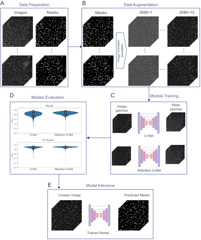
Figure 1: Workflow for the 3D segmentation of tubular structures in fluorescence microscopy images using U-Net and Attention U-Net models. (A) Data preparation: Schematic 2D sections of 3D fluorescence microscopy images of mouse liver tissue, showing the original images and corresponding binary masks. (B) Data augmentation: Simulation-based augmentation of the prepared data, generating images with varying signal-to-noise ratios (e.g., SNR = 15 and SNR = 1). (C) Model training: Patch-based training of U-Net and Attention U-Net models using both original and augmented data. Image and mask patches of size 64 x 64 x 64 are generated for training. (D) Model evaluation: Quantitative performance metrics, including Recall and F1 Score, are calculated for each model to assess segmentation accuracy on test datasets. (E) Model Inference: Application of the trained model on unseen images to generate predicted segmentation masks. Abbreviation: SNR = signal-to-noise ratio. Please click here to view a larger version of this figure.

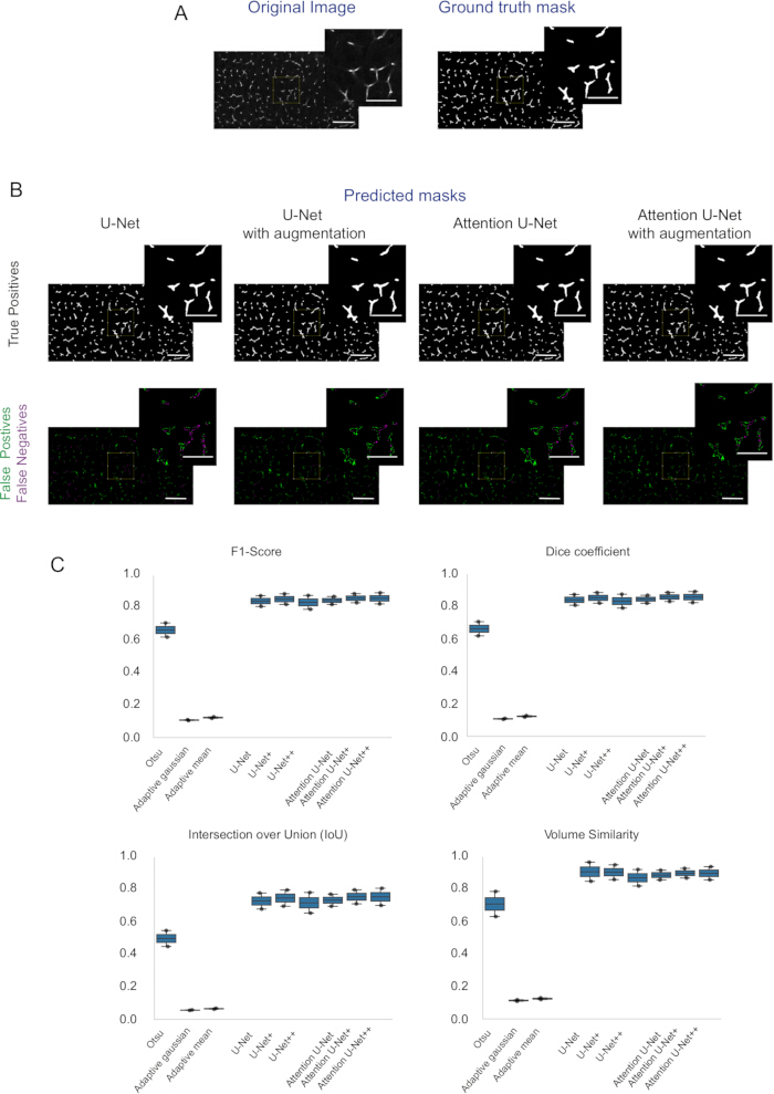
Figure 2: Evaluation of U-Net and Attention U-Net models for segmentation of Bile Canaliculi network from 3D fluorescence microscopy images of mouse liver tissue. (A) Representative 2D sections (middle section) of 3D fluorescence microscopy images, displaying the original image and the corresponding ground truth mask for BC in mouse liver tissue. The top-right images provide a zoomed-in view of the insets highlighted in each section. (B) Predicted segmentation masks generated by the U-Net, Attention U-Net, and their augmented versions. The upper row highlights True Positives (correctly segmented structures), the lower one shows False Positives (incorrectly identified structures), and False Negatives (missed structures) for each model. (C) Quantitative evaluation metrics for each model, including Accuracy, F1 Score, Precision, Recall, Volume Similarity, and Dice Coefficient. The evaluation was performed in the patches extruded from the 3D image. Error bars denote standard deviations across test images. Scale bar: 60 µm; inset scale bar: 30 µm. Abbreviation: BC = bile canaliculi. Please click here to view a larger version of this figure.

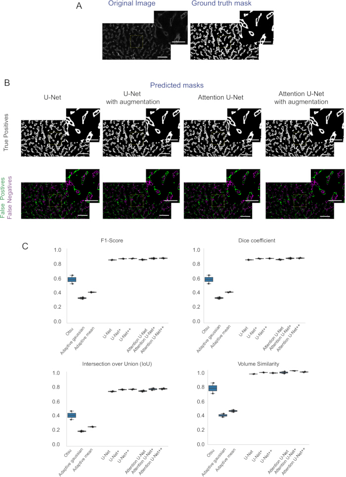
Figure 3: Evaluation of U-Net and Attention U-Net models for segmentation of the sinusoidal network from 3D fluorescence microscopy images of mouse liver tissue. (A) Representative 2D sections (middle section) of 3D fluorescence microscopy images, displaying the original image and the corresponding ground truth mask for Sinusoids in mouse liver tissue. The top-right images provide a zoomed-in view of the insets highlighted in each section. (B) Predicted segmentation masks generated by the U-Net, Attention U-Net, and their augmented versions. The upper row highlights True Positives (correctly segmented structures), the lower one shows False Positives (incorrectly identified structures), and False Negatives (missed structures) for each model. (C) Quantitative evaluation metrics for each model, including Accuracy, F1 Score, Precision, Recall, Volume Similarity, and Dice Coefficient. The evaluation was performed in the patches extruded from the 3D image. Error bars denote standard deviations across test images. Scale bar: 60 µm; inset scale bar: 30 µm. Please click here to view a larger version of this figure.

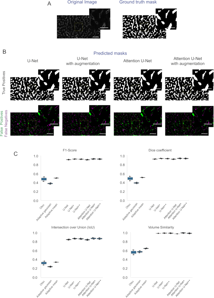
Figure 4: Evaluation of U-Net and Attention U-Net models for segmentation of the sinusoidal network from 3D fluorescence microscopy images of mouse liver tissue, considering the mask as filled tubes. (A) Representative 2D middle sections of 3D fluorescence microscopy images, displaying the original image and the corresponding ground truth mask for Sinusoids in mouse liver tissue. The top-right images provide a zoomed-in view of the insets highlighted in each section. (B) Predicted segmentation masks generated by the U-Net, Attention U-Net, and their augmented versions. Whereas the upper row highlights True Positives (correctly segmented structures), the lower one shows False Positives (incorrectly identified structures), and False Negatives (missed structures) for each model. (C) Quantitative evaluation metrics for each model, including Accuracy, F1 Score, Precision, Recall, Volume Similarity, and Dice Coefficient. The evaluation was performed in the patches extruded from the 3D image. Error bars denote standard deviations across test images. Scale bar: 60 µm; inset scale bar: 30 µm. Please click here to view a larger version of this figure.

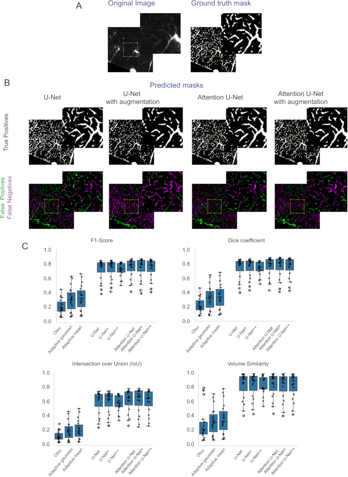
Figure 5: Evaluation of U-Net and Attention U-Net models for segmentation of the vascular network in mouse brain from 3D light-sheet microscopy images using filled-tube masks. (A) Representative 2D middle sections extracted from 3D light-sheet microscopy images of mouse brain, showing the original image and the corresponding ground truth mask for blood vessels. Zoomed-in views of selected insets are shown in the top-right corner of each panel. Predicted segmentation masks generated by U-Net, Attention U-Net, and their augmented versions. The top row highlights True Positives (correctly segmented vessel structures), while the bottom row illustrates False Positives (incorrectly segmented regions) and False Negatives (missed vessel structures) for each model. (C) Quantitative evaluation of model performance using metrics including Accuracy, F1 Score, Precision, Recall, Volume Similarity, and Dice Coefficient. Evaluations were performed on 3D patches extracted from the test volumes. Error bars represent standard deviations across the 19 test images. Please click here to view a larger version of this figure.

Video 1: Z-Stack animation of predicted masks for the BC network. The video shows an animated sequence through the z-stack of predicted segmentation masks for bile canaliculi in mouse liver tissue, generated by U-Net, Attention U-Net, and their augmented versions. Each 2D section highlights True Positives (white), False Positives (green), and False Negatives (magenta) for each model, moving through the entire stack. Abbreviation: BC = bile canaliculi. Please click here to download this Video.

Video 2: Z-Stack animation of predicted masks for the Sinusoidal network. The video shows an animated sequence through the z-stack of predicted segmentation masks for Sinusoids in mouse liver tissue, generated by U-Net, Attention U-Net, and their augmented versions. Each 2D section highlights True Positives (white), False Positives (green), and False Negatives (magenta) for each model, moving through the entire stack. Please click here to download this Video.

Video 3: Z-Stack animation of predicted masks for the Sinusoidal network as filled tubes. The video shows an animated sequence through the z-stack of predicted segmentation masks for the Sinusoidal network as filled tubes in mouse liver tissue, generated by U-Net, Attention U-Net, and their augmented versions. Each 2D section highlights True Positives (white), False Positives (green), and False Negatives (magenta) for each model, moving through the entire stack. Please click here to download this Video.

Video 4: Z-Stack animation of predicted masks for the brain vessels. The video shows an animated sequence through the z-stack of predicted segmentation masks for vessels, generated by U-Net, Attention U-Net, and their augmented versions. Each 2D section highlights True Positives (white), False Positives (green), and False Negatives (magenta) for each model, moving through the entire stack. Please click here to download this Video.

Table 1: Training time for U-Net 3D and Attention U-Net 3D Models on Bile Canaliculi and Sinusoid datasets with and without data augmentation. Training time for U-Net 3D and Attention U-Net 3D models on bile canaliculi and sinusoid datasets with and without data augmentation. The table lists the number of patches for each dataset and the corresponding training time in minutes. Data augmentation increases the number of patches from 1353 to 10824, leading to a significant increase in training time. The Attention U-Net model consistently requires more training time than the U-Net model, especially with augmented datasets, due to its additional complexity in focusing on relevant features within the data. Abbreviation: BC = bile canaliculi. Please click here to download this Table.

Table 2: Quantitative evaluation of U-Net 3D and Attention U-Net 3D models across four datasets using whole-image segmentation. This table reports the performance of each model as well as classical methods such as Otsu and adaptive thresholding, on four different datasets: bile canaliculi, sinusoidal networks (hollow and filled representations), and whole-brain vasculature, using whole 3D images for evaluation. For each combination of model and dataset, the number of test images is listed, along with performance metrics: Accuracy, Precision, Recall (Sensitivity), Specificity, F1 Score, Dice Coefficient, IoU, and Volume Similarity. These metrics provide a comprehensive assessment of segmentation quality in terms of both voxel-wise correctness and volumetric agreement between predictions and ground truth. Abbreviations: BC = bile canaliculi; IoU = Intersection over Union. Please click here to download this Table.

Table 3: Quantitative evaluation of U-Net 3D and Attention U-Net 3D models across four datasets using 64 x 64 x 64 patches. This table summarizes the performance of U-Net 3D and Attention U-Net 3D models on four datasets-bile canaliculi, sinusoidal networks (hollow and filled masks), and whole-brain vasculature-based on evaluation in 3D image patches of size 64×64×64 voxels. For each model-dataset combination, the number of test patches is listed alongside key performance metrics: Accuracy, Precision, Recall (Sensitivity), Specificity, F1 Score, Dice Coefficient, Intersection over Union, and Volume Similarity. These patch-level metrics offer localized insight into model performance and are especially useful for identifying spatially heterogeneous segmentation accuracy across volumes. Abbreviations: BC = bile canaliculi; IoU = Intersection over Union. Please click here to download this Table.

Supplemental Figure S1: Patch-level segmentation performance of 3D U-Net and Attention U-Net models for bile canaliculi segmentation. Graphs illustrate the quantitative performance of the 3D U-Net and Attention U-Net models on bile canaliculi datasets, evaluated using 3D image patches of size 64 x 64 x 64 voxels. Metrics shown include Accuracy, Precision, Recall (Sensitivity), Specificity, F1 Score, Dice Coefficient, Intersection over Union, and Volume Similarity. The results reflect variability across patches, offering localized insight into model performance and highlighting spatial heterogeneity within 3D liver tissue volumes. Abbreviations: BC = bile canaliculi; IoU = Intersection over Union. Please click here to download this File.

Supplemental Figure S2: Patch-level segmentation performance of 3D U-Net and Attention U-Net models for sinusoid segmentation. Graphs illustrate the quantitative performance of the 3D U-Net and Attention U-Net models on sinusoid datasets, evaluated using 3D image patches of size 64 x 64 x 64 voxels. Metrics shown include Accuracy, Precision, Recall (Sensitivity), Specificity, F1 Score, Dice Coefficient, Intersection over Union, and Volume Similarity. The results reflect variability across patches, offering localized insight into model performance and highlighting spatial heterogeneity within 3D liver tissue volumes. Abbreviation: IoU = Intersection over Union. Please click here to download this File.

Supplemental Figure S3: Patch-level segmentation performance of 3D U-Net and Attention U-Net models for sinusoids as filled tubes segmentation. Graphs illustrate the quantitative performance of the 3D U-Net and Attention U-Net models on sinusoids as filled tubes datasets, evaluated using 3D image patches of size 64 x 64 x 64 voxels. Metrics shown include Accuracy, Precision, Recall (Sensitivity), Specificity, F1 Score, Dice Coefficient, Intersection over Union, and Volume Similarity. The results reflect variability across patches, offering localized insight into model performance and highlighting spatial heterogeneity within 3D liver tissue volumes. Abbreviation: IoU = Intersection over Union. Please click here to download this File.

Supplemental Figure S4: Patch-level segmentation performance of 3D U-Net and Attention U-Net models for brain vasculature from light-sheet microscopy images. Graphs illustrate the quantitative performance of the 3D U-Net and Attention U-Net models on whole-brain vasculature datasets, evaluated using 3D image patches of size 64 x 64 x 64 voxels. Metrics shown include Accuracy, Precision, Recall (Sensitivity), Specificity, F1 Score, Dice Coefficient, Intersection over Union, and Volume Similarity. The results reflect variability across patches, offering localized insight into model performance and highlighting spatial heterogeneity within 3D liver tissue volumes. Abbreviation: IoU = Intersection over Union. Please click here to download this File.

Supplemental Figure S5: Overlay of segmentation results on original 3D fluorescence microscopy images of bile canaliculi. Representative image slices from 3D fluorescence microscopy datasets of bile canaliculi in mouse liver are shown with segmentation masks overlaid in red. Predicted masks from the 3D U-Net and Attention U-Net models are superimposed on the original grayscale microscopy images to visually assess segmentation accuracy. Ten example images are presented to illustrate the models' ability to capture diverse morphological features and handle signal variability across different tissue regions. Please click here to download this File.

Discussion

This protocol offers a simple yet powerful and accessible approach for deep learning-based segmentation of tubular structures in 3D fluorescence microscopy images, bridging the gap between technical complexity and usability in bioimage analysis. By integrating simulation-based data augmentation, interactive Jupyter notebooks, and efficient U-Net architectures, we provide an open-source tool capable of performing high-accuracy segmentation on complex tissue structures, such as bile canaliculi and sinusoidal networks. This toolbox addresses key challenges in 3D segmentation tasks, especially in handling data scarcity and variability in imaging conditions, making it a versatile addition to the bioimage analysis landscape.

A crucial component of our protocol is the simulation-based data augmentation, which enhances model performance even with a limited number of annotated images-a common limitation in biological studies. By generating augmented data that mimics realistic imaging artifacts, such as point spread function convolution, axial intensity decay, and Poisson and Gaussian noise, the toolbox produces models that are robust across a range of imaging conditions. This approach effectively increases data diversity, improving the generalizability of the models and providing a key advantage over traditional data augmentation techniques, which may not fully capture the heterogeneity present in biological specimens. However, this is limited by the morphological features intrinsically encoded in the initially provided mask. The reliance on pre-segmented masks for initial training data generation introduces potential biases if masks are not fully representative of the biological structures in question. Therefore, there is still an open question on how to generate realistic data augmentation in the morphological space, which can be potentially important to study tissues with alterations such as disease progression.

Our method uses two encoder-decoder models, 3D U-Net and Attention U-Net, selected for their high performance in biomedical imaging tasks. While the 3D U-Net provides a straightforward yet powerful segmentation architecture, the Attention U-Net improves precision by selectively focusing on relevant features and suppressing noise. Both models are included in the toolbox, allowing users to choose based on their specific dataset requirements. Our results show that the Attention U-Net model achieves higher performance metrics across datasets, particularly for challenging structures such as the sinusoidal network, where the added complexity of attention mechanisms helps mitigate the effects of low signal-to-noise ratios and structural variability. Nevertheless, it is important to note that the computational demands of the Attention U-Net are higher, which may affect its accessibility for users with limited GPU resources. Moreover, given the open-source nature of the pipeline, other more complex architectures can be easily added for future studies if required.

Our protocol offers an all-in-one, user-friendly pipeline that integrates essential steps for 3D segmentation in a single setup. This streamlined design is a key advantage, as it simplifies access to advanced segmentation tools without demanding expertise in programming or parameter adjustments. Additionally, our simulation-based data augmentation strategy enhances model robustness, reducing dependency on extensive manual annotations and improving model generalizability across diverse imaging conditions. In contrast to classical segmentation methods, which often rely on thresholding or region-growing algorithms that require careful fine-tuning^28,29 our deep learning approach requires minimal manual intervention. This contributes to democratizing high-quality, reproducible segmentation of complex 3D structures, making it accessible to a broader range of researchers, including those without extensive computational experience.

Beyond tubular networks, the flexibility of the protocol allows easy adaptation for segmenting other biological structures. Future enhancements could include the integration of self-supervised learning³⁰ or transfer learning³¹, which further reduces the need for annotated data while maintaining high segmentation accuracy. These strategies could also extend applicability to diverse imaging modalities, such as multiphoton or light sheet microscopy.

Despite its strengths, the protocol has several limitations that should be acknowledged. First, the dataset size remains relatively small, comprising only a few annotated volumes per structure. While data augmentation partially mitigates this issue, the risk of overfitting is still present, particularly when applying fine-tuned models to datasets with unseen variations in sample preparation or imaging conditions. Second, although our results indicate good generalization across different patches and animals, we have not yet tested the toolbox on datasets from other organs or microscopy modalities, which may exhibit distinct structural and noise characteristics. This limits the immediate generalizability of our approach. Finally, our evaluation strategy, while robust at the patch level, could benefit from additional metrics for topological consistency, which are relevant for network-like structures. Future work will address these limitations by expanding the dataset, incorporating domain adaptation techniques³², and evaluating the pipeline across broader biological contexts.

Summing up, this protocol represents an accessible and comprehensive solution for high-quality 3D segmentation of tubular structures in bioimaging. By combining effective model architectures, data augmentation strategies, and an interactive, user-friendly interface, our toolbox has the potential to expand the reach and impact of deep learning in bioimage analysis, enabling researchers worldwide to leverage these techniques in pursuit of a deeper understanding of biological structure and function.

Materials

List of materials used in this article

Name	Company	Catalog Number	Comments
Fiji			https://imagej.net/software/fiji/downloads
GitHub repository			https://github.com/hernanmorales-navarrete/3DMicroscopyImage Segmentation/tree/main
Labkit			https://imagej.net/plugins/labkit/
Zenodo repository			10.5281/zenodo.14029574

References

- Adler, M., Chavan, A. R., Medzhitov, R. Tissue biology: In search of a new paradigm. Annu Rev Cell Dev Biol. 39 (1), 67-89 (2023).
- Góra, A., Pliszka, D., Mukherjee, S., Ramakrishna, S. Tubular tissues and organs of human body-challenges in regenerative medicine. J Nanosci Nanotechnol. 16 (1), 19-39 (2016).
- Takahashi, K., et al. An analysis modality for vascular structures combining tissue-clearing technology and topological data analysis. Nat Commun. 13 (1), 5239(2022).
- Chen, B. C., et al. Lattice light-sheet microscopy: Imaging molecules to embryos at high spatiotemporal resolution. Science. 346 (6208), 1257998-1257998 (2014).
- Richardson, D. S., Lichtman, J. W. Clarifying tissue clearing. Cell. 162 (2), 246-257 (2015).
- França, C. M., et al. 3D-imaging of whole neuronal and vascular networks of the human dental pulp via CLARITY and light sheet microscopy. Sci Rep. 9 (1), 10860(2019).
- Nicolas, N., Dinet, V., Roux, E. 3D imaging and morphometric descriptors of vascular networks on optically cleared organs. iScience. 26 (10), 108007(2023).
- Friebel, A., et al. TiQuant: Software for tissue analysis, quantification and surface reconstruction. Bioinformatics. 31 (19), 3234-3236 (2015).
- Morales-Navarrete, H., et al. A versatile pipeline for the multi-scale digital reconstruction and quantitative analysis of 3D tissue architecture. eLife. 4, e11214(2015).
- Segovia-Miranda, F., et al. Three-dimensional spatially resolved geometrical and functional models of human liver tissue reveal new aspects of NAFLD progression. Nat Med. 25 (12), 1885-1893 (2019).
- Martínez-Torres, D., et al. Phenotypic characterization of liver tissue heterogeneity through a next-generation 3D single-cell atlas. Sci Rep. 14 (1), 2823(2024).
- Automatic recognition and characterization of different non-parenchymal cells in liver tissue. Morales-Navarrete, H., Nonaka, H., Segovia-Miranda, F., Zerial, M., Kalaidzidis, Y. 2016 IEEE 13th International Symposium on Biomedical Imaging (ISBI), , 536-540 (2016).
- Schneider, C. A., Rasband, W. S., Eliceiri, K. W. NIH Image to ImageJ: 25 years of image analysis. Nat Methods. 9 (7), 671-675 (2012).
- LeCun, Y., Bengio, Y., Hinton, G. Deep learning. Nature. 521 (7553), 436-444 (2015).
- Laine, R. F., Jacquemet, G., Krull, A. Imaging in focus: An introduction to denoising bioimages in the era of deep learning. Int J Biochem Cell Biol. 140, 106077(2021).
- Hallou, A., Yevick, H. G., Dumitrascu, B., Uhlmann, V. Deep learning for bioimage analysis in developmental biology. Development. 148 (18), dev199616(2021).
- Ronneberger, O., Fischer, P., Brox, T. U-Net: Convolutional networks for biomedical image segmentation. arXiv. , (2015).
- Oktay, O., et al. Attention U-Net: Learning where to look for the pancreas. arXiv. , (2018).
- Bettancourt, N., et al. Virtual tissue microstructure reconstruction across species using generative deep learning. PLoS One. 19 (7), e0306073(2024).
- Medical image computing and computer-assisted intervention. Lect Notes Comput Sci. Çiçek, Ö, Abdulkadir, A., Lienkamp, S. S., Brox, T., Ronneberger, O. 19th international conference, Athens, Greece, October 17-21, 2016, proceedings, part II, , 424-432 (2016).
- Vaswani, A., et al. Attention is all you need. arXiv. , (2017).
- Schlemper, J., et al. Attention gated networks: Learning to leverage salient regions in medical images. Med Image Anal. 53, 197-207 (2019).
- Sage, D., et al. DeconvolutionLab2: An open-source software for deconvolution microscopy. Methods. 115, 28-41 (2017).
- Arzt, M., et al. LABKIT: Labeling and segmentation toolkit for big image data. Front Comput Sci. 4, (2022).
- Napari contributors. napari: a multi-dimensional image viewer for python. , (2019).
- Chen, Y., Paetzold, J. C. 3D light-sheet microscopy data for SELMA3D 2024 challenge - Training subset with no annotations - whole brain images. BioStudies. , S-BIAD1197 (2024).
- Islam, M., Vibashan, V. S., Jose, V. J. M., Wijethilake, N., Utkarsh, U., Ren, H. Brain tumor segmentation and survival prediction using 3D attention UNet. arXiv. , (2021).
- Medical image computing and computer-assisted intervention. Lect Notes Comput Sci. Frangi, A. F., Niessen, W. J., Vincken, K. L., Viergever, M. A. MICCAI'98, first international conference, October 11-13, 1998, Cambridge, MA, USA, , 130-137 (1998).
- Otsu, N. A threshold selection method from gray-level histograms. IEEE Trans Syst Man Cybern. 9 (1), 62-66 (1979).
- Zhou, Z., Sodha, V., Pang, J., Gotway, M. B., Liang, J. Models genesis. Med Image Anal. 67, 101840(2021).
- Tajbakhsh, N., et al. Convolutional neural networks for medical image analysis: Full training or fine tuning. arXiv. , (2017).
- Wang, M., Deng, W. Deep visual domain adaptation: A survey. Neurocomputing. 312, 135-153 (2018).