Monitoring Conformational Dynamics of Single Unmodified Proteins using Plasmonic Nanotweezers

Summary

Plasmonic nanotweezers use localized surface plasmon resonance in gold nanostructures to trap single nanoparticles, including proteins, within a nanometer-scale optical field. Changes in the scattered signal reveal protein presence and conformational dynamics, enabling monitoring without fluorophore modifications or surface tethering.

Abstract

Current single-molecule techniques to characterize proteins typically require labels, tethers, or the use of non-native solution conditions. Such changes can alter protein biophysics and reduce the usefulness of the data acquired. Plasmonic nanotweezers is a technique that uses localized surface plasmon resonance (LSPR) on gold nanostructures to enhance the electric field within a confined hotspot region. This field enhancement allows for the use of low laser powers to trap single nanoparticles far smaller than conventional optical tweezers, down to only a few nanometers in diameter, such as single proteins. Trapping of single protein molecules within the hotspot region induces a shift in the local refractive index (n_protein > n_water), altering light scattering as a product of the molecule's polarisability, which is affected by its volume, shape anisotropy, and refractive index. An avalanche photodiode (APD) collects the subsequent changes in light scattering. These alterations can then be analyzed to determine changes in the trapped molecule, including its size, global conformation, and dynamics of conformational change over time. The incorporation of microfluidics within the system allows for controlled environmental changes and real-time monitoring of their subsequent effects on the molecule. In this protocol, we demonstrate the steps to trap single protein molecules, alter their environmental solution conditions, and monitor their corresponding conformational changes using a plasmonic nanotweezers system.

Introduction

Current single-molecule techniques for interrogating protein conformational dynamics include labelling-based methods such as fluorescence resonance energy transfer (FRET)^1,2, tethering-based approaches such as optical tweezers^3,4and atomic force microscopy (AFM)⁵, interference-based techniques such as interference scattering microscopy (iSCAT)⁶, or nanofluidic-based techniques such as nanopores^7,8,9. While these methods have many advantages; a few key limitations prevent them from providing data on unmodified protein conformational dynamics. FRET and optical tweezers require fluorophore labeling or tethering to a surface, which may affect the proteins' biophysical properties^10,11,12. iSCAT, although technically label-free, also requires interaction between the protein and a surface to observe interference generated between the two which potentially affects the proteins' properties. Moreover, limited by its signal-to-noise ratio, iSCAT can only detect proteins >40 kDa due to equipment noise and speckle-like background fluctuations¹³. Although this size limit can be alleviated through machine learning, buffer components are limited as they can affect optical properties, resulting in noisy data^13,14. Nanopores present fast translocation times of proteins through the pore (usually within 5 µs), rendering them unable to detect slower conformational dynamics^15,16, although research into alleviating these limitations, such as the use of DNA origami in a nanopore electro-osmotic trap¹⁷ or incorporation of plasmonics^18,19,20,21. Additionally, high salt concentrations, typically around 1 M, can reduce the applicability of the data for in vivo work^15,22. The ideal single-molecule technique for protein characterization should monitor proteins in real time and capture conformational dynamics over longer durations (i.e., milliseconds) without the need for modifications to the protein or non-native solution conditions.

Plasmonic nanotweezers are similar to conventional optical tweezers, in the sense that they use light to trap matter. Plasmonic nanotweezers, however, utilize localized surface plasmonic resonance (LSPR) to enhance the electric field by several orders of magnitude to generate a gradient force strong enough to trap single nanoparticles²³. Additionally, the trapped particle plays an active role in enhancing the strength of the trap, known as self-induced back-action (SIBA) trapping for nanoaperture structures²⁴. This SIBA trapping allows for low laser powers (i.e., milliwatts) to trap small particles down to only a few nanometers in diameter, such as proteins^25,26,27. Trapping single protein molecules within the hotspot region causes a shift in the local refractive index (n_protein > n_water), altering light scattering based on the molecule's polarizability which is influenced by the protein's volume, shape anisotropy, and refractive index²⁸. An avalanche photodiode (APD) then detects this information to monitor subsequent changes in light scattering. Moreover, plasmonic nanotweezers allow monitoring of the trapped proteins in real-time without labeling, tethers and harsh solution conditions for long time periods (i.e., minutes to hours)²⁹, fulfilling the criteria for an ideal single-molecule technique for proteins. Using a double nanohole (DNH) structure, plasmonic nanotweezers have demonstrated their ability to trap various proteins and elucidate key information from them including conformational transitions²⁹, disassembly kinetics³⁰, energy landscapes³¹, diffusion tracking³², and ligand binding^33,34. Besides DNH structures, alternative structure geometries have been demonstrated to trap particles with small particle sizes^35,36. In this protocol the fundamental steps to set up and run a plasmonic nanotweezers setup with an integrated microfluidics system are presented. We hope this protocol will help to increase the accessibility and understanding of plasmonic nanotweezers to researchers, particularly those in the structural biology and biophysics fields.

Protocol

CAUTION: Please read all relevant safety data sheets (SDS) for all chemicals used and adhere to all appropriate safety practices, and wear personal protective equipment (laser safety goggles, laboratory coats, gloves) as required.

1. Building the plasmonic nanotweezers setup

NOTE: The optical setup is based on the Modular Optical Tweezers System (OTKB) kit utilizing a different laser and APD (see Table of Materials). Only use optical equipment on a suitable optical table to reduce the impact of external vibrations on the system. The laser in the kit was 976 nm but as the peak resonance wavelength for the wedge resonance of the DNH structures is around 740-760 nm³³. We chose a NIR laser (852 nm) as it is close to the resonance peak, induces LSPR, and also has a better detection yield rate by the silicon-based APD. Lasers with longer²⁰ or shorter¹⁸ wavelengths have been used to trap biomolecules.

1. Set up the laser in the photodiode laser mount and feed it into a collimator, which leads to a collimated laser beam with width of 1.7 mm for our setup.
2. Add a half-wave plate to the light path to adjust the polarization. Adjust using a Glan-Taylor polarizer to ensure the vertical polarization (S-polarization) has the highest light intensity.
   ​NOTE: Using the correct polarization is vital to ensure maximum electric field enhancement from the DNH structures as they are polarization dependent.
3. Focus the light through a beam expander setup consisting of a plano-concave lens (f = -50 mm) followed by a plano-convex lens (f = 150 mm) to increase the beam width to around 5 mm to fill the full back aperture of the bottom objective.
4. Use a dichroic mirror (805 nm short pass) to reflect the laser to the desired location. Set up the camera (CCD) behind it.
5. Redirect the light into the bottom objective (100x/1.25 NA) and position the top objective (4x/0.1 NA) to the confocal distance to collect the transmitted light.
6. Add another dichroic mirror (805 nm short pass) to reflect the laser light towards the APD through a plano-convex lens positioned at its focal length to focus the light into the APD. Add the white light source (WLS) behind the dichroic mirror so it can pass back through the setup to reach the camera. Figure 1 shows a schematic of the fully assembled plasmonic nanotweezers setup.

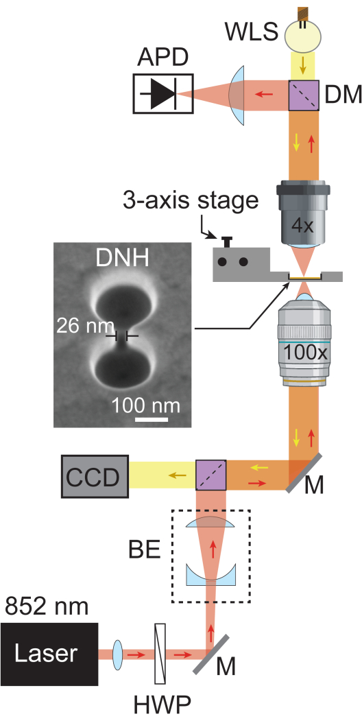
Figure 1: Plasmonic nanotweezers setup. The schematic shows the full optical pathway of the plasmonic nanotweezers setup. An 852 nm laser beam (red) passes through a collimator and a half-wave plate, then is expanded by the beam expander (BE) to ~5.1 mm. It is subsequently focused on the sample using a 100x objective. The transmitted laser light is collected by a 4x objective and recorded by an APD at a sampling rate of 1 MHz. White light from WLS (yellow) passes through the 4x objective, sample, and 100x objective before reaching the CCD, which provides a bright field image of the sample. Areas where both light paths cross are depicted in orange. SEM image of DNH taken at 20° tilt. Abbreviations: BE = Beam expander, CCD = Charge-coupled device, DM = Dichroic mirror, HWP = Half-wave plate, M = Silver mirror, and WLS = White light source. Please click here to view a larger version of this figure.

2. Fabricating the DNH structures

1. Deposit 5 nm Ti followed by 100 nm Au on a 550 µm thick fused silica wafer using e-beam evaporation as previously described^29,33. Dice the wafer to 1 cm x 1 cm samples ready for use.
   NOTE: E-beam evaporation was chosen as it produces a gold layer with low surface roughness, producing high-quality DNH structures with high trapping efficiency³⁷.
2. Take the blank gold film sample and mount it into a scanning electron microscope-focused ion beam (SEM-FIB) setup at room temperature using a gallium ion source.
3. Ensure FIB nanoapertures are aligned with SEM to produce DNH at accurate positions.
4. Create a marker box using a high-current ion beam (e.g., 100 pA). This marker will serve as a reference guide to locate the position of the DNH structures under the optical setup.
5. To create the DNH structure, two circles with a center-to-center distance of 200 nm and 160 nm diameter are bridged by a rectangle (3 nm x 40 nm). For a gap size of around 20-30 nm, etch circles with a dose factor of 0.09, while the rectangle dose is between 0.300 to 0.350 using a probe energy of 30 kV and beam current of 1 pA.
   NOTE: The SEM-FIB used has a resolution of 3 nm at this probe energy, allowing for reliable fabrication of DNH with gap sizes between 20-30 nm. We would not use a lower resolution as this will produce larger gap sizes, reducing the trapping efficiency of DNH. If a FIB is unfeasible, an alternative method for producing DNH structures is using polystyrene nanosphere lithography³⁸. Due to the high precision required to fabricate DNH structures, the same recipe may not produce the same gap size between SEM-FIB uses. Alter the dose and height of the rectangle (0.280 to 0.350 dose and 2 to 4 nm height) and measure the gap size, aiming for around 20 nm.

3. Coating of DNH samples

1. Use a solvent-resistant container, such as a crystallizing dish made of borosilicate glass 3.3, and add 20 mL of ethanol.
   CAUTION: Ethanol is highly flammable and an irritant. Use in a fume-hood only. Store in a cool, well-ventilated place. Handle with gloves and a laboratory coat.
2. Weigh 32 mg of Poly(ethylene glycol) methyl ether thiol (PEG-thiol; average molecular weight 800 g/mol) and mix this into the ethanol, ensuring all PEG-thiol has dissolved to produce a solution with a concentration of around 2 mM to maximize the monolayer density³⁹.
   CAUTION: PEG-thiol is an irritant; handle it with appropriate PPE.
3. Add the sample chips containing the nanostructures to the mixture using straight tweezers, cover, and incubate overnight (~16 h) at room temperature for the PEG-thiol to form a self-assembled monolayer on the gold surface.
4. After incubation, rinse samples by holding them with straight tweezers over a suitable container in the fume-hood. Use a squirt bottle to spray ethanol on each side thoroughly. Dry fully using an air gun before subsequent storage or mounting in the plasmonic nanotweezers.
   NOTE: Samples can be stored at 4 °C to improve longevity as they can degrade overtime.

4. Mounting the PEG coated sample into a flow cell

1. Place the coated sample into the 3D printed flow cell (printed by a Form 2 printer with Clear V4 resin) using straight tweezers with the gold layer facing upwards (see Supplementary Figure 1 for key parameters and values in our flow cell design).
2. Peel one side of the clear PET plastic double-sided tape cover using straight tweezers and place it on the sample and flow cell, ensuring the nanostructures and intake/outtake holes in the flow cell remain uncovered. Gently press around the edges of the tape with rounded tweezers to ensure it has properly adhered to the flow cell and sample.
3. Peel the other side of the tape off and gently place a glass coverslip (thickness 0.17 mm) over the sample using rounded tweezers. Gently press around the edges of the coverslip with the rounded tweezers to ensure it has properly adhered. This creates a liquid channel (height = 50 µm, volume = 3.5 µL) within the flow cell.
   NOTE: Do not press the coverslip at or near where the nanostructures are located as they may become damaged. If the coverslip is dirty, wash it with ethanol and dry it with an air gun before mounting.
4. Mix equal parts of A and B of the duplicating silicone solutions at a 1:1 ratio (or as per the manufacturers instruction) onto a microscope slide using a small pipette tip.
5. Fill the gaps between the coverslip and flow cell with the mixed duplicating silicone, gently pushing it under the coverslip. Hold the flow cell upside down and carefully place duplicating silicone around the inner wall of the hole before using the pipette tip to gently move it onto the visible edges of the fused silica underside of the sample (See Supplementary Figure 2).
6. Leave to dry with the gold layer facing upwards until the duplicating silicone has fully set, according to the manufacturer's instructions.
   NOTE: Take care not to allow silicone to cover nanostructures when applied on the underside of the sample. Take care not to force the duplicating silicone under the coverslip as it may enter the intake/outtake holes of the flow cell or the nanostructures, which can be difficult to clean (Supplementary Figure 3).

5. Connecting the microfluidics system

NOTE: Ensure the use of clean tubing for the system. Here, small ID PTFE tubing: 0.18 mm ID and large ID PTFE tubing: 0.8 mm will be used, but other ID values will work.

1. Set up the syringe pump and connect it to the 3/2-way solenoid valve using the large PTFE tubing. Connect one port of the valve to the buffer container and the other to a holding coil, around 1 mL in volume, made from the large ID tubing to prevent backflow into the syringe.
   NOTE: The 3/2 valve can be controlled through a valve controller, which determines whether the solution is infused/withdrawn from the buffer container or from the holding coil.
2. Connect the holding coil to the center valve of the 12/1 rotary bidirectional microfluidic valve. Connect containers for solutions using small ID tubing for scarce or valuable samples and large ID tubing for the rest. Use one valve only for infusing into a waste container and another only for infusing into the flow cell; use small ID tubing for the flow cell infusion valve.
3. Connect large ID tubing from the output of the flow cell to the waste container. Figure 2 shows a schematic of the fully connected microfluidic system.
   ​NOTE: Small ID PTFE tubing is preferable for the intake of the flow cell and for valves that will be used for protein infusion due to the smaller volume where the sample will remain in the tubing. Large ID PTFE tubing is preferable for less expensive or more abundant materials such as buffers. Try to use minimal tubing to reduce this dead volume further.

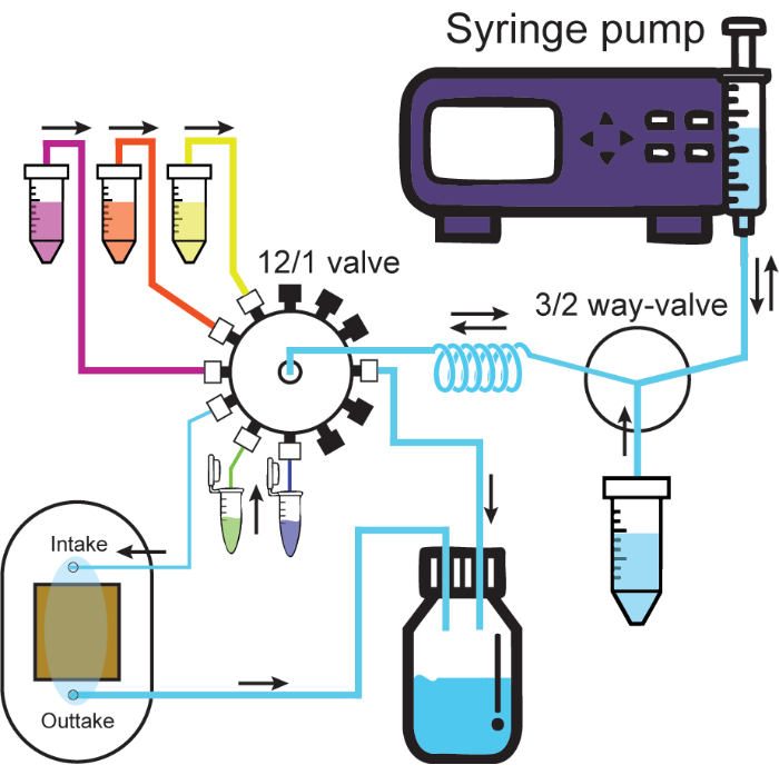
Figure 2: Microfluidic system. Schematic illustrates the microfluidic system. The syringe pump infuses or withdraws solutions through one port of the 3/2-way valve, either the solution container or the holding coil. Solutions connected to the 12/1 valve always go through the holding coil when withdrawn and can then be infused through the desired channel. Infusion to the intake channel connected to the flow cell will push out the solution from the flow cell into the waste container. Thick and thin tubes represent large and small ID tubing from protocol. Black caps on the 12/1 valve represent sealed channels. Flow directions are labeled by black arrows. Please click here to view a larger version of this figure.

6. Preparing microfluidics system

1. Load up the microfluidics system UI on the PC and check the components are properly connected. Select the play icon next to the wire and distributor to open their respective UI. To bypass the 3/2-way valve, turn port 1 on the wire.
2. Ensure valves that will be used within the system are cleaned by infusing isopropanol (IPA) and then wash tubing multiple times with buffer(s) of choice or distilled water to remove air and IPA within the system. Infusion can be done by selecting the desired valve on the distributor UI and running the syringe pump, selecting infuse/withdraw, and choosing the desired volume and flow rate (e.g., 0.5 mL volume and 0.2 mL/min flow rate).
   NOTE: Do not infuse IPA into flow cells, as this will degrade the cell and the glue, which may lead to leaks.

7. Mounting flow cell into plasmonic nanotweezers and checking for leaks

1. Attach the inlet and outlet tubes to the appropriate part of the flow cell before placing them on clean tissue with a gold layer facing upwards.
2. Infuse buffer into the flow cell with a high flow rate (~0.3 mL/min) and check that fluid moves across the sample in the flow cell and that no fluid is visible on the flow cell exterior or underside. Higher flow rates can be used, provided no leaking occurs. If the sample leaks unmount and remount.
3. Add 1-2 drops of immersion oil onto the 100x objective before placing the flow cell into the plasmonic nanotweezers stage with the gold layer facing downwards. Place metal clips over the flow cell magnets and lock the stage to help keep it in place.
   CAUTION: Objective oil is an irritant, health hazard, and toxic to aquatic life, only handle with gloves.

8. Locating nanostructures on sample

1. Turn on the white light source. Open the camera software and increase the gain and exposure time until the nanostructures are visible. Turn on the laser with relatively high laser power and adjust the z-axis manually until the laser spot is visible. Prioritize increasing exposure time and gain over increasing the laser power to find the laser spot.
   CAUTION: Lasers pose a serious potential risk to users. Ensure appropriate PPE such as laser safety goggles with sufficient optical density within the required wavelength range are used.
2. Turn on the piezoelectric controller and select the appropriate settings for the COM port and max voltage. Set the values for the x-, y- and z- axes to half the max voltage to allow for a good range to align the stage in all directions.
   NOTE: The COM port of the piezoelectric controller can be found and changed in the device manager under the ports tab.
3. Move the laser spot to overlay with one of the DNH using the main stage x-, y- and z-axes control knobs. Ensure the APD is turned on and then gently close the enclosure to the plasmonic nanotweezers.
   NOTE: Using a marking tool in the camera software, if available, will help to move the laser spot over a nanostructure. Set the marker to the center of the laser spot and turn the laser off, but leave the white light source on, to allow for easier alignment to a nanostructure. The APD can be oversaturated and damaged if too much laser light reaches it. Ensure sample is in the way of the laser path and gradually increase laser power to ensure saturation is not reached. Neutral density (N.D) filters can be placed before the APD to reduce the light that reaches it if necessary.

9. Optimally aligning the laser with the desired nanostructure

1. Open the software associated with the APD recording, such as a homemade Labview UI, and set the cut-off frequency to 1 kHz. Name and set the desired file path and the naming format of the files that will be saved.
2. Turn the white light source off and turn the laser back on. Set to an appropriate laser power (e.g., ~20 mW) and use the piezoelectric controls to adjust the x-, y- and z-axes until the APD signal is as high as possible, avoiding APD saturation and with minimal standard deviation (S.D.) of the trace.
   NOTE: The APD will likely have an optimal sensitivity range for transmission (see product manual) which is ideal to stay around, e.g., 1000-2000 mV. N.D. filters can be used to keep the transmission around this range. The main consideration is for the transmission to not be close to the APD saturation point, as trapping may increase the transmission to the saturation limit, leading to loss of data.

10. Infusing proteins into the flow cell

1. Turn the laser off to preserve the lifespan of the nanostructures and run the syringe pump control unit and the distributor UI to set the valve and withdraw the desired amount of protein (e.g., 30 µL). For withdrawing using the small ID tubing, a lower flow rate helps to ensure all solutions are withdrawn (~0.01 - 0.1 mL/min). Higher flow rates can be used to reduce the time spent waiting if desired.
   NOTE: The optimal volume of protein to use depends on how valuable the protein is and what the experiment hopes to achieve. The typical protein concentration we use is 1 µM and an aliquot volume of 100 µL. If the protein sample is abundant, higher concentrations can be used to reduce average trapping time. However, if concentrations are too high, the risk of trapping two of the same proteins within the nanostructure will increase. If the experiment requires an infusion of a different ligand/protein after trapping the initial protein, a lower aliquot volume may be preferred to minimize waste and the time taken to infuse the next solution. Ensure tubing remains submerged in solution to prevent air from entering the system. Special care should be taken for protein aliquots if the tubing does not reach the bottom of the container or the solution is over-withdrawn.
2. Using the microfluidics UI, infuse the protein solution at a similar flow rate to the withdrawal rate (~0.01 - 0.1 mL/min). Allow to infuse at this rate until the protein solution reaches the flow cell, then reduce the flow rate to ≤0.001 mL/min. Check the volume and time on the syringe pump to make sure they match the expected volume (e.g., 1 min for 1 mL volume at 1 mL/min).
   NOTE: The required volume for this can be calculated based on the volume of the tubing from the microfluidic system to the flow cell. If the length and ID of the tubing are known, an online calculator for the volume of a cylinder can be used. The infusion rate can be adjusted as desired, e.g., >0.001 mL/min for protein infusion to reduce the average waiting time for a trap. However, caution is advised as if the flow rate is too high, this may prevent proteins from entering the nanostructure.

11. Collecting data

1. While the protein solution is being infused into the flow cell, start data recording of the APD signal. Adjust the x-, y- and z-axes as necessary using the piezoelectric controller UI, as the system will likely drift over time. Ideal trapping traces have a consistent general pattern following that of the trace in Figure 3.
2. Upon observing a large change in transmission and S.D. similar to the exemplar trapping trace, note down the time this occurs for future data sorting (See Figure 4B for example .).
   NOTE: Drifting in the system can lead to changes in the transmission and an increase in S.D., sometimes quite suddenly, which could be mistaken for a protein trap. Ensure the signal jump displays the same pattern as the exemplar trap and no external interference was present when the jump occurred, such as aligning drift or loud noises being picked up by the system.
3. If the protein needs to be released as part of the experiment, turn the laser off for ~5 s and turn it back on. The trace should have a large change in transmission and a significantly lower S.D., indicating a return to the baseline state.
   NOTE: If a large change in transmission and/or S.D. is not observed, or a similar trace to the protein being trapped is observed, the protein is likely stuck to the sample surface (see Figure 5B, for example).

12. Unmounting the sample

1. After performing the desired experiment, turn off the laser, take the flow cell out of the 3-axis stage, and disconnect the microfluidic system tubing.
2. Place the flow cell on clean tissue with the gold layer of the sample facing upwards. Using a scalpel, carefully cut the glue under the glass coverslip and gently lift it off with rounded tweezers. Dispose of it in the designated broken glass bin.
   CAUTION: Broken glass and the use of sharp objects can cause injury. Ensure safety goggles, gloves, and a lab coat are worn.
3. Hold the flow cell at an angle with the gold layer still facing upwards and use rounded tweezers to carefully remove the glue on the underside of the flow cell to free the sample. Duplicating silicone allows for easy removal without damaging the DNH structures.
4. Using straight tweezers, pick up the sample and rinse thoroughly with IPA, then water before drying with an air gun. If reusable, store the sample in a suitable container with the gold layer facing upwards.
   NOTE: Samples typically have a usable span of around 1-2 weeks if handled properly, although the size of nanostructures changes over time. If overly damaged, switch to a fresh sample for the next experiment. Damage can be in the form of scratches present on the gold surface near the nanostructures or from poor experimental performance, indicating degradation of the nanostructures²⁹.

13. Preparing the system for future use

1. Use folded lens tissue to wipe the oil off the objective in one direction, lifting it off and repeating it with another clean part of the tissue.
   NOTE: Objectives are prone to smudging and scratches, which can significantly impair performance. Always wear gloves during cleaning and avoid touching organic material. Use only new lens-cleaning tissue to prevent contamination and clean in a single direction with one motion. Avoid rubbing the lens and cleaning tissue back and forth to minimize damage. If dry cleaning is insufficient, apply a small amount of ethanol to the tissue, wipe the oil off as previously mentioned, and finish with dry tissue.
2. If the same protein/buffer solutions will be used next, the tubing may not need to be changed. If different solutions are used, replace the tubing to reduce the risk of contamination from previous solutions.
   NOTE: Do not use the same tubing for more than 1 week, even if performing experiments with the same solutions, as it will get dirty over time.

Results

Following data acquisition, data analysis can be performed on the raw data using MATLAB code to generate traces from the raw data collected by the APD. Figure 3 depicts an exemplar trapping trace including the baseline before trapping, the trapping event where a large change in transmission (ΔT/T₀) and standard deviation is observed before the laser is turned off for around 5s before being turned back on. A significant reduction in standard deviation and return of transmission to similar levels as the baseline indicates the release of protein. Linear drift is removed from the trace using the MATLAB function detrend.m, and then the mean value of the data is added back to the detrended trace. Occasionally, we need to detrend the trace as the setup drifts over time, causing a linear decrease in transmission (see the grey trace in Figure 3). Small changes in the baseline traces before and after trapping are due to stage adjustment to optimize the baseline with minimal standard deviation, demonstrated in Figure 4A. Sometimes, protein molecules are visible in the trace without being trapped, termed passing-by proteins. Proteins passing by appear as a sharp change in transmission, similar to a typical trap (Figure 4B), but with a significantly shorter duration, as shown in Figure 4A. Power spectral density (PSD) presents another analysis to confirm protein trapping by providing signal strength at various frequencies. Protein conformational motions are typically seen in the >1 µs range by single molecule spectroscopy methods⁴⁰. Figure 4C demonstrates that compared to the baseline, trapping a protein leads to higher signal strength, at least within the 10 kHz range (> 100 µs). It also highlights the importance of aligning the stage to an optimized baseline, as a bad baseline could increase the noise at frequencies between 50-500 Hz, a frequency range overlaid with protein conformational motions.

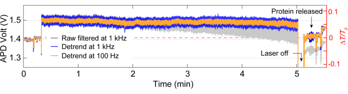
Figure 3: Full trapping trace for a single protein. Representative trace for a full trap, including the baseline, trapping a protein, and release of the protein. Jumps in trace before and after trapping are due to alignment. Please click here to view a larger version of this figure.

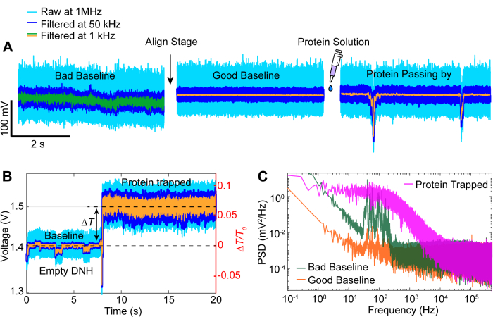
Figure 4: Common trace events. (A) Examples of an alignment from a bad to a good baseline and a protein passing close to the hotspot. (B) Trapping trace showing the process from the baseline when the DNH hotspot is empty to when the protein is trapped. (C) Power spectral density (PSD) plot between the good and bad baselines depicted in (A) and the protein trapped in (B). Higher PSD values indicate greater noise at particular frequencies. Please click here to view a larger version of this figure.

Most trapping events follow the same general pattern as the trace in Figure 3, although occasional issues may arise during experiments. For most experiments, the protein should be released manually by turning the laser off once the desired experiment is completed. In some cases, however, the protein can leave the trap without intervention, as shown in Figure 5A. Conversely, sometimes proteins can remain at the trapping site even after turning the laser off, likely due to the protein sticking to the sample. This sticking results in a noisy trace after turning the laser off and on (see Figure 5B). The likelihood of this occurring depends on the protein, as some proteins are more prone to surface adsorption^41,42. The use of a coating such as PEG-thiol can reduce the chances of protein sticking^39,43. Unless desired, such as studying protein-protein interactions, another issue is double trapping, where a second protein is trapped after the first trap. This is characterized by another sharp increase in transmission, similar to the first trap, and a change in standard deviation (see Figure 5C).

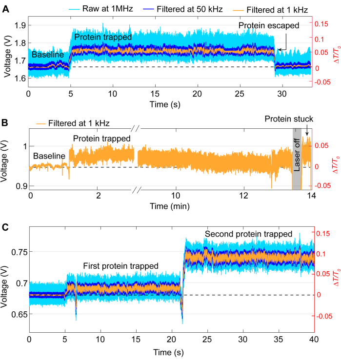
Figure 5: Examples of undesirable trapping events. (A) Unintended release of a protein from the DNH hotspot. (B) Example of protein becoming stuck on the sample surface in the DNH hotspot. (C) Trace jump occurs when a second protein is trapped whilst the first still remains in the DNH hotspot. Please click here to view a larger version of this figure.

A representative experiment carried out on in situ iron loading to an apo-ferritin molecule demonstrates the use of plasmonic nanotweezers as a tool to investigate protein conformational dynamics²⁹. Ferritin is an iron carrier protein that exists in two states: apo-ferritin, which contains no iron, and holo-ferritin, which is filled with iron^44,45. Ferrous iron enters the protein through 3-fold channels where it is oxidized to ferric iron and stored in the protein core⁴⁶. Figure 6A depicts a typical trapping trace of apo-ferritin with a ferrous solution infused for over 20 min while the protein is trapped. The 20 s traces taken along the whole trace at points b-e provide insight into the changes occurring to the protein over time. In Figure 6B, apo-ferritin is trapped in a standard PBS buffer, and no significant changes are observed in the trace. Figure 6C, D show fluctuations in the S.D of the traces, which are caused by iron loading into the protein through its 3-fold channels, resulting in a more dynamic state (apo-) where the channels are open, and a more compact state (holo-) with the channels closed. Upon the ferritin molecule being filled with iron, it transitioned to its holoform, resulting in a stable trapping trace, as shown in Figure 6E. Probability density functions (PDF) in Figures 6B-E further showcase the changes the protein undergoes upon exposure to different solution conditions over time.

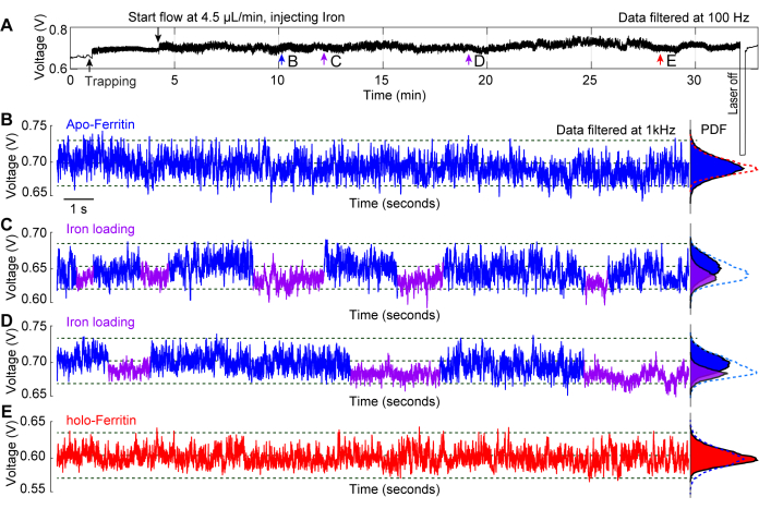
Figure 6: In situ iron loading into a trapped apoferritin. (A) Full transmission trace of a DNH with an apoferritin molecule trapped, followed by injecting a ferrous solution to the trapping site to observe ferritin's conformational changes associated with iron loading. (B) 20-s trapping trace of an apoferritin trapped before ferrous solution reached hotspot. (C, D) 20-s trapping traces after the apoferritin molecule was exposed to the ferrous solution. Blue and purple segments mark the higher and lower S.D of the trace, indicating flexible and rigid conformations of ferritin, respectively. (E) 20-s trapping trace after apoferritin was exposed to the ferrous solution for >20 minutes. Probability density function (PDF) plots on the right show the distribution of transmission and are color-coded to the blue and purple segments. This figure has been modified from²⁹. Please click here to view a larger version of this figure.

Supplementary Figure 1: Gold DNH sample mounted on the 3D printed flow cell. The sample is placed into a special slot and adhered to the flow cell using double-sided PET adhesive tape. Key parameters and associated measurements for our flow cell design are labeled. Please click here to download this File.

Supplementary Figure 2: Back of flow cell with gold DNH sample mounted and inner wall labelled. The sample is sealed in the flow cell using duplicating silicone. Please click here to download this File.

Supplementary Figure 3: Diagram of the flow cell with gold DNH mounted with intake and outtake holes labeled. Please click here to download this File.

Discussion

A crucial step in the protocol is ensuring the flow cell does not leak before being set into the stage, which should be tested outside of the mount at a high flow rate beforehand. Leakage after the sample is mounted can damage optical components, in particular the bottom objective.

The alignment may drift from its optimal position over time during an experiment, causing signal variation due to the sensitivity of the plasmonic nanotweezers. When this occurs, realign using the piezoelectric controls to maximum transmission and minimum standard deviation of the baseline, as a noisy baseline reduces the quality of data. Care should be taken to make meticulous notes of when alignments are made to remove the risk of confusing user interference for a trapping event. If major drifting occurs, gently align the stage to minimize the risk of releasing the protein and note the time of adjustment.

Modifications and alterations to the presented technique can be made based on specific experimental needs. For example, a temperature-controlled stage can help cool/heat the sample as desired instead of using laser heating to increase the temperature^31,33. Other techniques, for example, interferometric scattering microscopy (iSCAT), can provide interference of the protein within the scattering field of the DNH, obtaining additional signal proportional to the polarizability of the protein, which is associated with particle size^47,48.

Plasmonic nanotweezers are purely a temporal sensing technique as data is recorded by the APD (a single-pixel detector). This technique provides no direct information on the structural changes of a protein, such as which regions of the protein are involved in a conformational change or where a ligand or another protein may bind to the protein. Additionally, the technique is limited to a temporal range of >1 µs due to the sampling rate of the data acquisition card (1 MHz). Considering the Nyquist frequency, where the highest possible range is half the acquisition rate, in this case, 2 µs under perfect conditions.

In this protocol, we have described the process of setting up a plasmonic nanotweezers experiment to trap a single protein and monitor changes in its conformational dynamics over time. The technique can be developed on any home-built or commercial microscope. Contrary to fluorescence or tethering-based approaches, such as smFRET and optical tweezers, the technique can trap proteins without labels or tethers and still achieve single-molecule sensitivity. The solution conditions can be changed whilst the protein is trapped using a microfluidics system, allowing for real-time monitoring of the effect of different solutions on the protein. These features make plasmonic nanotweezers a promising tool within the biophysics and biosensing fields, particularly for proteins that conventional techniques struggle to interrogate in their native states. Future applications will focus on decoding the conformational dynamics of more dynamic proteins such as intrinsically disordered proteins and proteins containing intrinsically disordered regions, and membrane proteins, whose dynamics and even structure elude current techniques.

Materials

List of materials used in this article

Name	Company	Catalog Number	Comments
100x Objective (NA = 1.25)	Olympus	PLN100XO	Clean oil only with lens cleaning tissue in one motion
12-1 rotary bidirectional microfluidic valve	Elveflow
3/2 way solenoid valve	Elveflow
4x Objective (NA = 0.1)	Olympus	PLN4XP
Airgun	RS Components	666-6772
Avalanche photodiode (APD)	Thorlabs	APD120A/M	Do not oversaturate, 50 MHz bandwidth, static sensitive
Butterfly laser diode	Thorlabs	FPL852S
Charge-coupled device (camera)	Hikrobot	MV-CE200-10UC
Crystallising dish	VWR	216-0065
Data acquisition card	National instruments	USB-6361	2 MHz sampling rate
Double-sided tape	Adhesive Research Inc	ARcare92712	Cut appropriate shape for flow cell with a laser cutter
Ethanol			Fume hood only, use gloves
Fibreport collimator	Thorlabs	PAF2-A7B
Glass microscope coverslips (thickness 0.17 mm)
Half wave plate	Thorlabs	AHWP10M-980
Ideal-tek 120 mm, stainless steel, straight tweezers	RS Components	282-7472	For holding sample and peeling double sided tape
Isopropanol (IPA)			Fume hood only, use gloves
Lens cleaning tissue	Thorlabs	MC-5
Metrosil rapid duplicating silicone parts A and B	Metrodent	MSILR/1
Microscope slides (75 mm x 26 mm)
Modular Optical Tweezers System	Thorlabs	OTKB/M-CUSTOM
Objective oil	Olympus		Use gloves, store between 2oC-8oC
Photodiode laser mount	Thorlabs	CLD1015
Piezoelectric controller	Thorlabs	MDT693B
Piezoelectric stage	Thorlabs	Nanomax 300
Planoconcave lens (f = -50 mm)	Thorlabs	LC1715-B
Planoconvex lens (f = 150 mm)	Thorlabs	LA1433-B
Planoconvex lens (f = 60 mm)	Thorlabs	LA1134-B
Poly(ethylene glycol) methyl ether thiol (PEG-thiol) 800 MW	Sigma Aldrich	729108	Store between 2oC-8oC
PTFE tubing (ID: 0.18 mm)	Vici Jour	JR-T-6805-M25
PTFE tubing (ID: 0.8 mm)	Cole-Parmer	WZ-21942-72
SEM-FIB	Zeiss	Crossbeam 550	Gallium ion source
Shortpass dichroic mirror 805 nm	Thorlabs	DMSP805
Silver mirror	Thorlabs	PF-10-03-P01
Syringe pump	Harvard Apparatus	70-4511
Weller Erem 120 mm stainless steel, flat, rounded tweezers	RS Components	176-1150	For holding glass coverslip and peeling glue from flow cell

References

- Peter Lu, H. P. Sizing up single-molecule enzymatic conformational dynamics. Chem Soc Rev. 43 (4), 1118-1143 (2014).
- Mazal, H., Haran, G. Single-molecule FRET methods to study the dynamics of proteins at work. Curr Opin Biomed Eng. 12, 8-17 (2019).
- Ritchie, D. B., Woodside, M. T. Probing the structural dynamics of proteins and nucleic acids with optical tweezers. Curr Opin Str Biol. 34, 43-51 (2015).
- Neupane, K., Solanki, A., Sosova, I., Belov, M., Woodside, M. T. Diverse metastable structures formed by small oligomers of α-Synuclein probed by force spectroscopy. PLoS One. 9 (1), e86495(2014).
- Hughes, M. L., Dougan, L. The physics of pulling polyproteins: a review of single molecule force spectroscopy using the AFM to study protein unfolding. Rep Prog Phys. 79 (7), 076601-076601 (2016).
- Young, G., et al. Quantitative mass imaging of single biological macromolecules. Science. 360 (6387), 423-427 (2018).
- Schmid, S., Dekker, C. Nanopores: a versatile tool to study protein dynamics. Essays Biochem. 65 (1), 93-107 (2021).
- Van Meervelt, V., et al. Real-time conformational changes and controlled orientation of native proteins inside a protein nanoreactor. J Am Chem Soc. 139 (51), 18640-18646 (2017).
- Awasthi, S., Ying, C., Li, J., Mayer, M. Simultaneous determination of the size and shape of single α-Synuclein oligomers in solution. ACS Nano. 17 (13), 12325-12335 (2023).
- Sµnchez-Rico, C., Von Vithenberg, L., Warner, L., Lamb, D. C., Sattler, M. Effects of fluorophore attachment on protein conformation and dynamics studied by spFRET and NMR spectroscopy. Chemistry. 23 (57), 14267-14277 (2017).
- Yin, L., et al. How does fluorescent labeling affect the binding kinetics of proteins with intact cells. Biosens Bioelectr. 66, 412-416 (2015).
- Berkovich, R., et al. Rate limit of protein elastic response is tether dependent. Proc Natl Acad Sci. 109 (36), 14416-14421 (2012).
- Dahmardeh, M., Mirzaalian Dastjerdi, H., Mazal, H., Köstler, H., Sandoghdar, V. Self-supervised machine learning pushes the sensitivity limit in label-free detection of single proteins below 10 kDa. Nat Meth. 20 (3), 442-447 (2023).
- Becker, J., et al. A quantitative description for optical mass measurement of single biomolecules. ACS Photon. 10 (8), 2699-2710 (2023).
- Houghtaling, J., et al. Estimation of shape, volume, and dipole moment of individual proteins freely transiting a synthetic nanopore. ACS Nano. 13 (5), 5231-5242 (2019).
- Plesa, C., et al. Fast translocation of proteins through solid state nanopores. Nano Lett. 13 (2), 658-663 (2013).
- Schmid, S., Stömmer, P., Dietz, H., Dekker, C. Nanopore electro-osmotic trap for the label-free study of single proteins and their conformations. Nat Nanotechnol. 16 (11), 1244-1250 (2021).
- Shi, X., Verschueren, D. V., Dekker, C. Active delivery of single DNA molecules into a plasmonic nanopore for label-free optical sensing. Nano Lett. 18 (12), 8003-8010 (2018).
- Verschueren, D. V., et al. Label-free optical detection of DNA translocations through plasmonic nanopores. ACS Nano. 13 (1), 61-70 (2019).
- Verschueren, D., Shi, X., Dekker, C. Nano-optical tweezing of single proteins in plasmonic nanopores. Small Meth. 3 (5), 1800465(2019).
- Peri, S. S. S., et al. Quantification of low affinity binding interactions between natural killer cell inhibitory receptors and targeting ligands with a self-induced back-action actuated nanopore electrophoresis (SANE) sensor. Nanotechnology. 32 (4), 045501(2020).
- Leong, I. W., Tsutsui, M., Yokota, K., Taniguchi, M. Salt gradient control of translocation dynamics in a solid-state nanopore. Anal Chem. 93 (49), 16700-16708 (2021).
- Juan, M. L., Righini, M., Quidant, R. Plasmon nano-optical tweezers. Nat Photon. 5 (6), 349-356 (2011).
- Juan, M. L., Gordon, R., Pang, Y., Eftekhari, F., Quidant, R. Self-induced back-action optical trapping of dielectric nanoparticles. Nat Phys. 5 (12), 915-919 (2009).
- Pang, Y., Gordon, R. Optical trapping of 12 nm dielectric spheres using double-nanoholes in a gold film. Nano Lett. 11 (9), 3763-3767 (2011).
- Pang, Y., Gordon, R. Optical trapping of a single protein. Nano Lett. 12 (1), 402-406 (2012).
- Kotnala, A., Gordon, R. Quantification of high-efficiency trapping of nanoparticles in a double nanohole optical tweezer. Nano Lett. 14 (2), 853-856 (2014).
- Booth, L. S., et al. Modelling of the dynamic polarizability of macromolecules for single-molecule optical biosensing. Sci Rep. 12 (1), 1995(2022).
- Yousefi, A., et al. Optical monitoring of in situ Iron loading into single, native ferritin proteins. Nano Lett. 23 (8), 3251-3258 (2023).
- Yousefi, A., et al. Structural Flexibility and Disassembly Kinetics of Single Ferritin Molecules Using Optical Nanotweezers. ACS Nano. 18 (24), 15617-15626 (2024).
- Peters, M., et al. Energy landscape of conformational changes for a single unmodified protein. NPJ Biosens. 1 (1), 14-14 (2024).
- Peters, M., McIntosh, D., Branzan Albu, A., Ying, C., Gordon, R. Label-free tracking of proteins through plasmon-enhanced interference. ACS Nanosci Au. 4 (1), 69-75 (2024).
- Ying, C., et al. Watching single unmodified enzymes at work. arXiv. , (2021).
- Yang-Schulz, A., et al. Direct observation of small molecule activator binding to single PR65 protein. NPJ Biosensing. 2 (1), 1-10 (2025).
- Yang, W., van Dijk, M., Primavera, C., Dekker, C. FIB-milled plasmonic nanoapertures allow for long trapping times of individual proteins. iScience. 24 (11), 103237(2021).
- Koya, A. N., et al. Novel plasmonic nanocavities for optical trapping-assisted biosensing applications. Adv Optical Mater. 8 (7), 1901481(2020).
- Goswami, A., Umashankar, R., Gupta, A. K., Aravindan, S., Rao, P. V. Development of a microstructured surface using the FIB. J Micromanufact. 1 (1), 53-61 (2018).
- Onuta, T. D., Waegele, M., DuFort, C. C., Schaich, W. L., Dragnea, B. Optical field enhancement at cusps between adjacent nanoapertures. Nano Lett. 7 (3), 557-564 (2007).
- Al-Ani, A., et al. The influence of PEG-thiol derivatives on controlling cellular and bacterial interactions with gold surfaces. Appl Surf Sci. 462, 980-990 (2018).
- Schuler, B., Hofmann, H. Single-molecule spectroscopy of protein folding dynamics-expanding scope and timescales. Curr Opin Str Biol. 23 (1), 36-47 (2013).
- Kopac, T. Protein corona, understanding the nanoparticle-protein interactions and future perspectives: A critical review. Int J Biol Macromol. 169, 290-301 (2021).
- Li, X., Guo, W., Xu, R., Song, Z., Ni, T. The interaction mechanism between gold nanoparticles and proteins: Lysozyme, trypsin, pepsin, γ-globulin, and hemoglobin. Spectrochim Acta A Mol Biomol Spectrosc. 272, 120983(2022).
- Emilsson, G., et al. Strongly stretched protein resistant poly(ethylene glycol) brushes prepared by grafting-To. ACS Appl Mater Inter. 7 (14), 7505-7515 (2015).
- Theil, E. C., Liu, X. S., Tosha, T. Gated pores in the ferritin protein nanocage. Inorg Chim Acta. 361 (4), 868-874 (2008).
- Theil, E. C., et al. The ferritin iron entry and exit problem. Inorg Chim Acta. 297 (1), 242-251 (2000).
- Takahashi, T., Kuyucak, S. Functional properties of threefold and fourfold channels in Ferritin D=deduced from electrostatic calculations. Biophys J. 84 (4), 2256-2263 (2003).
- Gemeinhardt, A., et al. Label-free imaging of single proteins secreted from living cells via iSCAT microscopy. J Vis Exp. (141), e58486(2018).
- Piliarik, M., Sandoghdar, V. Direct optical sensing of single unlabelled proteins and super-resolution imaging of their binding sites. Nat Comm. 5 (1), 4495(2014).
Reprints and Permissions