Development of a Microfluidics-Based Approach for Investigating Microtubule Polymer Mechanics

Summary

This protocol details the design and fabrication of a microfluidic device suitable for investigating microtubule polymer mechanics. The synthesis of microfabrication, automated flow control, and computational modeling techniques enables a flexible system ideally suited for probing the cellular cytoskeleton in vitro.

Abstract

In this protocol, we describe the design and fabrication of a microfluidic device developed for the investigation of microtubule polymer mechanics. The design utilizes the intrinsic benefits of Polydimethylsiloxane (PDMS)-based microfluidic devices and introduces several features to enable a robust and customizable high-throughput experimental approach. The developed device incorporates redundant bubble-trapping capabilities to prevent the occurrence of detrimental air bubbles. Furthermore, the device interfaces with an automated flow control system to reduce manual intervention and enable high-throughput analyses. Commercial simulation software is utilized to better develop and understand the fluid transport using this system. Finally, we demonstrate the capability to conduct multiple experiments simultaneously within a single device by growing microtubule extensions with distinct fluorescent labels in different sections of the device. Overall, this microfluidic flow system can be used to probe microtubule polymer mechanics and provides improvements in experimental design for broader microtubule in vitro studies. The synthesis of microfabrication, automated flow control, and computational modeling approaches enables a flexible system ideally suited for probing the cellular cytoskeleton in vitro.

Introduction

Microfluidics enables precise control of miniscule fluid volumes, often less than one microliter, by the intricate design and fabrication of fluid-flow channels^1,2. The small scale of microfluidic devices gives rise to unique engineering phenomena. Namely, the Reynolds number-a dimensionless measure of the ratio between inertial and viscous forces in fluid flow-is small, typically on the order of O(10) or lower in microfluidics, underscoring the importance of viscous forces in microfluidic devices. Additionally, the Péclet number, which compares convective to diffusive transport, shows that convective transport is generally negligible in microfluidics^3,4,5. This diffusion-driven, laminar flow regime in microfluidics is advantageous, as it supports parallel experiments on a single device by maintaining precise fluid gradients.

Photolithography remains the primary method for fabricating microfluidic devices^6,7,8. In brief, this process involves creating a 'master' etched template of the microfluidic design (Figure 1). A photosensitive substrate is prepared, and a photomask of the microfluidic design selectively exposes areas of photoresist to ultraviolet radiation. Subsequent etching methods develop the substrate, producing a relief of the design. Polydimethylsiloxane (PDMS) is often cast and cured onto the master. The cured PDMS, which adopts the negative features of the design, is then removed from the master and bonded to a glass coverslip. This entire fabrication process typically takes 1-2 days, enabling quick design iterations and the production of multiple devices. Detailed reviews of soft lithography and microfabrication processes are available in other references^{1,2,3,10,11,12,13}.

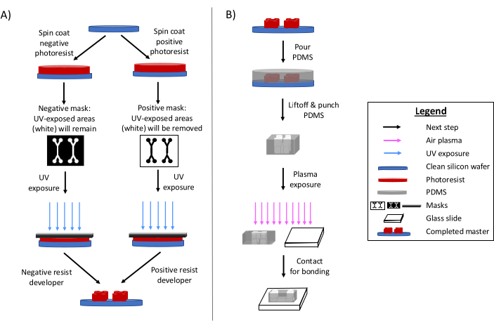
Figure 1: Overviews of the traditional photolithography process and microfabrication process. (A) Traditional photolithography process and (B) microfabrication process. Depending on the application and desired photoresist characteristics, a negative or a positive photoresist can be used, even though they will yield the same design master. Characteristics such as feature height desired or photoresist melting temperature help determine the appropriate photoresist type. This figure has been modified with permission from Rogers (2022)¹⁴. Please click here to view a larger version of this figure.

The use of microfluidics has expanded the possibilities in many research fields, with its most recent impact being in the biological sciences. Given its small scale, microfluidics allows for the precise management of limited, valuable resources such as cells or proteins. Even more impactful is the tunability of microfluidic systems to mimic physiological conditions, such as modifications in substrate stiffness, the exertion of force on a specimen, and even the integration of electrical current. Additionally, the use of microfluidics offers the ability to manipulate multiple reagents in parallel and to rapidly prototype and iteratively refine system designs. These features enable the miniaturization of entire laboratory workflows onto a single device, commonly referred to as a "lab-on-a-chip"^{1,6,9,15,16,17,18,19}.

One of the cell-biological applications of microfluidics is investigation of microtubule polymers. Microtubules are an essential component of the cell's cytoskeleton, playing a vital role in processes such as cell division and intracellular cargo transport^20,21. As the most rigid element of the cytoskeleton, microtubules exhibit an elastic modulus comparable to that of Plexiglass^22,23. Their robust mechanical properties are crucial for various cellular functions, including, for example, cardiomyocyte contraction, where they cyclically bend and relax during the heart's systolic and diastolic phases²⁴. Microfluidic devices have been previously adopted to investigate the properties of microtubules and their higher-order structures in vitro. Indeed, microfluidics has been used to probe microtubule polymerization dynamics, microtubule-microtubule interactions, and the effects of microtubule-associated proteins on microtubule mechanical properties^{25,26,27,28,29,30,31,32,33,34,35,36,37,38,39,40,41}.

While the introduction of microfluidics into the microtubule field has brought about many exciting discoveries, room for improvement still lies in the adaptation of these devices for microtubule research. In this work, we address two specific limitations that persist in studying microtubules in microfluidic devices: the potential for air bubble formation within the device, typically introduced by manual manipulation of microfluidic devices, and the underutilization of high-throughput assays. First, manual manipulations, such as plugging and unplugging tubing, can introduce bubble formation into channels. Air bubble formation within a flow cell is catastrophic, as air bubbles can denature proteins, shear microtubule polymers, and adversely affect cell cultures^42,43. In addition, sharp corners and oblique angles in the device result in non-uniform surface wetting, increasing the possibility of air entrainment. Numerous techniques have been developed to reduce the formation, persistence, and impact of air bubbles; however, the use of bubble mitigation methods is not universal^{42,43,44,45,46}. Furthermore, although one of the major advantages of using microfluidics is the ability of high-throughput experimentation, microfluidics has not yet been used to scale-up microtubule research. Microfluidic devices can be designed to test multiple experimental conditions in parallel on the same device. For example, fluid gradients can be used to direct the flow of different microtubule-associated proteins or drugs, enabling their targeted delivery to specific regions of partitioned microtubules within the same device.

Here, we iteratively designed a microfluidic device that addresses these limitations. We provide the step-by-step protocol of the fabrication of the device, thereby enabling a wider audience to employ microfluidic technology in their microtubule research. This device design incorporates bubble-trapping features and utilizes an automated flow control system to reduce manual intervention while also enabling gradients of solutions in the device for high-throughput analyses. In summary, the development of this microfluidic design can facilitate broader research and understanding of microtubule mechanics while offering valuable improvements to experimental designs across the broader microtubule research field.

Protocol

NOTE: The work detailed in this portion of the protocol was performed in the Vanderbilt Institute of Nanoscale Science and Engineering (VINSE) core Class 100 cleanroom. A controlled cleanroom with appropriate gowning and UV-filtered lighting is desired to prevent device damage due to humidity/ambient lighting conditions and to prevent particulate contamination. All manipulations on silicon wafers should be done with the silicon wafer polished side facing up. Use tweezers when manipulating wafers and minimize touching surfaces of the wafer to prevent scratching. Keep wafers in Petri dishes with the lids covered when transporting and at the end of each day unless otherwise directed.

1. Photolithography (6 - 8 h)

1. Plasma clean a 3" silicon wafer for 5 min under vacuum (ideally, vacuum pressure < 5 × 10^-5 torr) using either oxygen (O₂) or clean dry air (CDA) plasma.
2. Center the silicon wafer onto a spin coater for deposition of the photoresist.
3. Deposit ~1-2 mL of SPR 220 7.0 photoresist onto the center of the silicon wafer.
   CAUTION: Handle photoresist with gloves and eye protection and dispose of according to manufacturer/site-specific protocols.
4. Spin-coat the photoresist on the silicon wafer to the desired thickness based on manufacturer spin curves. Generate ~13 µm thick layers by spinning at 1000 RPM for 30 s. Later, clean the residual photoresist on the spin coater with acetone and dispose of it per site-specific protocols.
   NOTE: If after spin-coating, the wafer is not uniformly coated with photoresist, repeat steps 1.2-1.4. A non-uniform coating could be due to a non-centered wafer on the spin coater, using too little photoresist, and/or not depositing the photoresist onto the center of the wafer.
5. While touching as little of the photoresist on the wafer as possible, transfer the silicon wafer to a hot plate set at 70 ˚C.
6. Incubate the silicon wafer on the hot plate, increasing the temperature by 10 ˚C every 3-5 min until the temperature reaches 115 ˚C.
7. Turn off the hot plate and allow the silicon wafer to cool until its temperature is below 65 ˚C.
   NOTE: The heating and cooling steps are performed slowly to prevent thermal cracking of the photoresist, which is common at this thickness. If thermal cracks do occur, they can usually be rectified by re-heating the silicon wafer and slowing the rate of cooling.
8. Using forceps, transfer the cooled silicon wafer to a mask aligner and load both the silicon wafer and a corresponding photomask into the mask aligner following the manufacturer/site-specific protocols.
   NOTE: Photomasks were manufactured by an external party using a specified design, which was created with AutoCAD. See Supplementary File 1 for the mask design rendering.
9. Expose the silicon wafer to ultraviolet (UV) radiation for a specific time (based on the power of the UV lamp) following the manufacturer/site-specific protocols. The desired energy for this application is ~400 mJ/cm², and calculate the exposure time by the formula: .
10. After exposure, remove the silicon wafer from the mask aligner and allow the photoresist to rehydrate for 4 h by air circulation. Ensure the Petri dish lid is left off to allow for air circulation, but place the dish in an area unlikely to be exposed to particulates.
    NOTE: A 4-h break can be taken during this rehydration time, but it is recommended to continue with the procedure on the same day.
11. After the 4-h rehydration, transfer the exposed wafer to a hot plate set at 70 ˚C.
12. Incubate the silicon wafer on the hot plate, increasing the temperature by 10 ˚C every 3-5 min until the temperature reaches 115 ˚C.
13. Allow the wafer to incubate at 115 ˚C for 10 min.
14. Create an insulating 'cover' for the exposed wafer by molding a sheet of aluminum foil in the shape of a Petri dish lid.
15. Turn off the hot plate and cover the exposed wafer with the aluminum foil cover. Allow the wafer to cool ambiently overnight.
    NOTE: Thermal cracking of the photoresist is much more common during the post-exposure incubation step, which is why a slow cooling overnight is recommended. This completes the steps required for the first day of fabrication. It is recommended to proceed to the next section the following day.

2. Development (1 - 2 h)

1. When ready to develop the exposed wafer, obtain a clean container and an appropriate photoresist developer. Here, MF-319 developer is used with a dedicated container.
   CAUTION: Handle the developer with gloves and eye protection, transfer the bulk container to a secondary container, and dispose of it according to manufacturer/site-specific protocols.
2. Pour enough developer into the container to fully submerge the exposed wafer (actual volume will vary based on the container).
3. Submerge the exposed wafer in the developer and wait until all unwanted photoresist has been dissolved. Gently swirling/agitating the container aids in development until little-to-no residual photoresist is visible on the wafer other than the device design.
   NOTE: Multiple changeouts of the developer solution may be required to fully remove the undesired photoresist, depending on the volume of developer solution used.
4. Remove the developed wafer from the development solution and gently rinse both sides of the wafer with de-ionized (DI) water for 30 s.
5. Dry the developed wafer with nitrogen (N₂) gas.
6. Store the developed wafer in a Petri dish in a dry, cool environment until ready for further use. Wrap the Petri dish in aluminum foil to prevent degradation of the photoresist due to exposure to ambient light.
   NOTE: It is recommended, but not required, to proceed to the next section the same day.

3. Silanization (1 - 2 h)

1. Transfer the silicon wafer to a desiccator.
2. Place a small aluminum container (or a piece of aluminum foil folded into a container shape) in the desiccator.
3. Pipet 1 drop (~50 µL) of trichloro(1H, 1H, 2H, 2H-perfluorooctyl) silane into the aluminum container.
   CAUTION: Handle silane solution with gloves and eye protection and dispose of it according to manufacturer/site-specific protocols.
4. Close the desiccator and turn on the vacuum.
5. Allow desiccation/silanization to occur for 1-2 h.
6. After the silanization time has finished, turn off the vacuum and retrieve the silanized wafer. Store the silanized wafer in an aluminum foil-wrapped Petri dish in a dry, cool environment until ready for further use.
   NOTE: Silanization may need to be periodically repeated on the wafers and more frequently on devices where thinner layers of PDMS are used. If PDMS adhesion is noticed when removing the PDMS from the wafer, the wafer may need to be re-silanized, and this section should be repeated once all PDMS has been removed from the wafer. This completes the steps required for creating microfluidic device masters. The masters are stable and subsequent sections can be executed when desired.

4. PDMS deposition (1 - 2 h)

NOTE: If there is residual PDMS on the master from a previous microfabrication, the residual PDMS must be removed prior to depositing new PDMS.

1. On a scale, weigh into a container PDMS and associated curing agent in a 10:1 weight ratio. The total weight required will vary depending on the desired PDMS thickness and Petri dish size. For a 4" Petri dish, ~20 g of PDMS and ~2 g of curing agent will yield a thickness of 2-3 mm.
   CAUTION: Handle PDMS solution with gloves and eye protection and dispose of it according to manufacturer/site-specific protocols.
2. Mix the PDMS and curing agent in the container for 5 min using a plastic spatula or other appropriate tool.
3. Transfer the mixed PDMS container to a desiccator for degassing.
4. Close the desiccator and turn on the vacuum. Air bubbles will begin to appear in the PDMS.
5. Allow desiccation/degassing to occur for 30 min. Depending on the amount of PDMS used and the container shape, the actual time may vary; a general endpoint is when few to no bubbles are present in the PDMS.
6. After degassing, turn off the vacuum and retrieve the PDMS container.
7. Pour the mixed and degassed PDMS onto the master in a Petri dish.
8. Incubate the master in the closed Petri dish at 65 ˚C overnight to allow PDMS to fully cure.
   NOTE: This completes the steps for PDMS deposition. It is recommended to allow the PDMS to cure in an incubator overnight. The PDMS is then stable, so subsequent sections can be executed when desired.

5. PDMS device assembly (1 - 2 h)

1. Retrieve the device master(s) that have cured PDMS, a pair of forceps, a standard 1.5 mm biopsy punch with a manual plunger, and a scalpel/razor blade.
   CAUTION: Handle the blade with care and never cut toward yourself or others. A self-retracting or safety blade is recommended.
2. Around the device features, cut out rectangular pieces of PDMS from the layer master. Ensure each piece of PDMS has some room on each side, flanking the device features to facilitate good bonding contact while ensuring that each piece fits on its own 22 mm × 22 mm glass coverslip.
   NOTE: It is important to avoid touching the bottom surface of the PDMS (the side with the features), so always handle the PDMS by the edges using tweezers. Additionally, never place the feature side of the PDMS facing down on any surface. When not in use, store the PDMS with the feature side facing up in a closed container until needed.
3. Punch inlet and outlet holes in the pieces of PDMS using a clean 1.5 mm hole punch. Punch through the device PDMS into a spare layer of sacrificial PDMS rather than into a hard surface that could damage the hole punch.
4. Retrieve and clean a 22 mm × 22 mm glass coverslip with an isopropyl alcohol (IPA) wetted wipe.
5. Plasma clean the 22 mm × 22 mm coverslip for 5 min under vacuum (pressure < 0.5 Torr) using CDA plasma. This will remove any debris or organic coatings on the coverslip.
6. Wipe the 22 mm × 22 mm glass coverslip and the feature side of the PDMS with an IPA-wetted wipe.
7. Place both the PDMS (feature-side facing up) and the glass coverslip (the same side facing up as was cleaned before) into the plasma cleaner and plasma clean simultaneously for 30 s under vacuum (pressure < 0.5 Torr) using CDA plasma.
8. Remove both the glass coverslip and the PDMS device from the plasma cleaner. Invert the PDMS so that the feature side is facing down and place it onto the glass coverslip. Observe bonding and lightly press on the PDMS as needed to facilitate good contact.
9. Incubate the bonded coverslip in a closed Petri dish at 65 ˚C for 3 min to facilitate bonding.
   NOTE: Plasma bonding changes the hydrophobicity of the glass coverslip, generating a hydrophilic surface. It has been observed through anecdotal evidence that the original hydrophobic state of the coverslip returns after approximately 2 days of incubation at room temperature. It is recommended to use fabricated devices no earlier than 2 days after plasma bonding. This completes the microfabrication steps. The devices have no set shelf life but should be stored in a cool, dry area when not in use.

6. Microfluidic flow channel preparation (1 h)

1. Secure an assembled microfluidic device into a clean custom stage adapter⁴⁷.
2. Retrieve a syringe, a Lour-lock adapter and fitting ferrule, and a piece of 1.5 mm outer diameter transparent tubing (approximately 15-20 cm long). Connect the tubing to the syringe via the adapter.
3. Connect three more pieces of tubing to the microfluidic device outlets (this tubing does not need to be a specific length) and direct the other end of these tubings into a waste vial downstream.
4. Using the syringe, prepare the microfluidic device by introducing solutions according to the steps below. The sequence and volume of solutions are as follows: 50 µL of BRB80 buffer solution, 25 µL of anti-rhodamine antibody solution, wait for 5 min, 50 µL of BRB80, 25 µL of poloxamer 407 (F127), wait for 15 min, and 50 µL of BRB80. See Table 1 for an example.
   1. Draw the solution from its source into the tubing.
      NOTE: Do not pull the solution all the way into the syringe itself. The solution should remain only in the tubing.
   2. Gently press down on the syringe plunger until a small droplet of fluid is present at the end of the tubing. This will prevent any air from entering the microfluidic device when the tubing is attached.
   3. Attach the tubing to the inlet of the microfluidic device.
   4. Slowly press down on the syringe plunger until most, but not all, of the solution has flown through the tubing. Leaving a small amount of liquid in the tubing will ensure that no air is inadvertently forced through the tubing. Observe the tubing and microfluidic channels during these transfers, looking for any bubbles.
      NOTE: If bubbles occur in the tubing, begin troubleshooting (try to remove the bubble prior to it entering the microfluidic device by unplugging the tubing just before the bubble arrives and then re-attaching the tubing after the bubble passes, etc.).
   5. Repeat steps 6.4.1-6.4.4 for the next reagent until all reagents have been flown through. A new piece of inlet tubing will be needed for each reagent to prevent cross-contamination of source reagents. Once the final BRB80 wash is complete, the device is stable for several min. A drop of BRB80 solution on the inlets will prevent the drying out of the device.
5. Prepare guanosine-5'-[(α,β)-methyleno]triphosphate (GMPCPP)-stabilized microtubule 'seeds' according to standard protocols (with a TTR labeling ratio of ~25%)^47,48.
6. Prepare an imaging buffer solution ('antifade') at a 2x working concentration by combining the following reagents in respective quantities (depending on stock concentrations) to yield their specified final concentrations: BRB80 supplemented with 40 mM glucose, 40 µg/mL glucose oxidase, 16 µg/mL catalase, 0.5 mg/mL casein, 50 mM potassium chloride, and 10 mM dithiothreitol (DTT). This imaging buffer is used to prolong photostability. See Table 2 for an example.
7. Dilute a portion of the 2x antifade solution 1:1 in BRB80 to yield a 1x working solution of antifade. Warm this antifade to room temperature (RT); the stock antifade solution should be kept on ice.

Order	Reagents	Volume Dilution	Wash Volume	Incubation Time
1	BRB80	N/A	50 μL	N/A
2	Anti-rhodamine antibody	1:50 in BRB80, mix well	25 μL	5 min
3	BRB80	N/A	50 μL	N/A
4	Poloxamer 407 (F127)	1% in BRB80	25 μL	15 min
5	BRB80	N/A	50 μL	N/A

Table 1: Order of preparation of microfluidic device channels.

Volume	Reagent	Stock Concentration	Final Concentration
16 μL	D-Glucose	2 M	80 mM
16 μL	Glucose Oxidase	2 mg/mL	80 μg/mL
16 μL	Catalase	0.8 mg/mL	32 μg/mL
14 μL	Casein	28 mg/mL	0.16 mg/mL
8 μL	DTT	1 M	20 mM
40 μL	Potassium Chloride	1 M	100 mM
290 μL	BRB80	1x	N/A
400 μL	FINAL (2x working concentration)

Table 2: Antifade imaging solution recipe (2x concentration).

7. Introduction of microtubule seeds to microfluidic (10 - 15 min)

1. Connect the microfluidic device to the microscope.
   NOTE: Because microtubule stability is temperature-dependent, it is recommended for the imaging experiments to be conducted at 35 °C.
2. Attach 10-15 cm of new tubing to the syringe and draw a desired dilution of GMPCPP-stabilized microtubule seeds into the tubing.
   NOTE: For this device, ~10 nM GMPCPP-microtubule seeds was the optimal concentration.
3. Gently press down on the syringe plunger until a small droplet of fluid is present at the end of the tubing. This will prevent any air from entering the microfluidic device when the tubing is attached.
4. Attach the tubing to the inlet of the microfluidic device.
5. Slowly press down on the syringe plunger until most, but not all, of the solution has flown through the tubing. Leaving a small amount of liquid in the tubing will ensure that no air is inadvertently forced through the tubing.
6. Detach the inlet tubing from the microfluidic device and syringe and attach a new piece of tubing to the syringe.
7. Draw BRB80 into the tubing.
8. Repeat steps 7.3-7.6 to wash out non-bound microtubule seeds from the device.
9. Observe the attachment of seeds to the microfluidic surface using total internal reflection fluorescence (TIRF) microscopy. The ideal number of seeds in a single field of view will vary based on the application and the field of view size, but generally, ~10-20 seeds per 80 µm × 80 µm field of view is optimal. Repeat steps 7.2-7.9 as needed until the desired seed density is reached.
   NOTE: For monitoring the microtubule seed density, intermittent short-light exposure (100 ms) should be used since no antifade is yet present in the solution.
10. Once the appropriate bound seed density is reached, attach a new piece of inlet tubing to the syringe.
11. Draw warm 1x antifade solution into the tubing and repeat steps 7.3-7.6.
    NOTE: With the antifade solution now in the device, the photostability is significantly improved, and the device is stable. However, it is still recommended to minimize the exposure to laser light.

8. Growing microtubule extensions from seeds (15 - 30 min)

1. Combine fluorescently labeled tubulin, unlabeled tubulin, 2x antifade solution, Guanosine-5'-triphosphate (GTP), and BRB80 to achieve a final solution containing 14 µM tubulin at a 7% fluorescent labeling ratio, antifade at a 1x working concentration, and 1 mM GTP.
   NOTE: If using different concentrations or different labeling percentages of tubulin, the volume of each reagent will need to be adjusted to achieve the desired final concentration and labeling ratio. Keep the tubulin solution on ice until ~30 s before introduction, at which point, take the solution off the ice and warm it in hand to RT. This will aid in the polymerization of microtubule extensions, which is a temperature-dependent process. Indeed, microtubule polymerization should be carried out at 35 °C, while all other experimental steps can be conducted at RT.
2. Attach 10-15 cm of new tubing to the syringe and draw tubulin solution into the tubing.
3. Gently press down on the syringe plunger until a small droplet of fluid is present at the end of the tubing. This will prevent any air from entering the microfluidic device when the tubing is attached.
4. Attach the tubing to the inlet of the microfluidic device.
5. Slowly press down on the syringe plunger until most, but not all, of the solution has flown through the tubing. Leaving a small amount of liquid in the tubing will ensure that no air is inadvertently forced through the tubing. Detach the inlet tubing from the microfluidic device.
6. Image at the desired frequency for 10-15 min or until extensions are long enough to bend. Typically, imaging is performed at 488 nm every 5 s and 561 nm every 60 s until extensions are at least 5-10 µm long (~15 min).
   NOTE: At this concentration of tubulin, the microtubules may stochastically switch between periods of polymerization and depolymerization; this is to be expected, but overall, the microtubule extensions will elongate⁴⁹.

9. Stabilizing microtubule extensions (10-15 min)

1. Combine Taxol, 2x antifade solution, and BRB80 to achieve a final solution containing 10 µM taxol and antifade at a 1x working concentration.
   NOTE: Keep the taxol solution on ice until ~30 s before introduction, at which point take the solution off the ice and warm it in hand to RT. This will prevent depolymerization of microtubule extensions, which is a temperature-dependent process.
2. Attach 10-15 cm of new tubing to the syringe and draw taxol solution into the tubing.
3. Gently press down on the syringe plunger until a small droplet of fluid is present at the end of the tubing. This will prevent any air from entering the microfluidic device when the tubing is attached.
4. Attach the tubing to the inlet of the microfluidic device.
5. Press down on the syringe plunger until most, but not all, of the solution has flown through the tubing. Leaving a small amount of liquid in the tubing will ensure that no air is inadvertently forced through the tubing.
6. Repeat steps 9.2-9.5 twice in rapid succession. The same piece of tubing may be used in this instance.
   NOTE: Taxol promotes de novo microtubule nucleation from tubulin in solution, and these microtubules can land on the surface of the microfluidic channel and interfere with subsequent imaging/bending. Because of this, the taxol solution should flow through the device rapidly and in multiple iterations to remove as much free tubulin from the device as quickly as possible.
7. Verify that microtubules grown from seeds are still present and stabilized in the device.

10. Bending stabilized microtubule extensions (10 - 15 min)

NOTE: Stabilized microtubule extensions can now be bent using a flow controller. Here, a regulated, positive-pressure displacement system (Elveflow OB1 MK3+) was used to flow the solution from an airtight source vial through a flowmeter and into the microfluidic. Depending on the specifics of the available flow controller setup, modifications may be made to the following steps.

1. Set up flow controller and associated equipment per manufacturer/site-specific protocols, using tubing to connect the source vial to the flowmeter inlet and the flowmeter outlet to the microfluidic inlet, but do not attach the tubing to the microfluidic device yet.
2. Insert ~200 µL of the 10 µM taxol solution into a source vial that can be attached to the flow controller setup. This setup uses Luer-lock connections to create an airtight seal.
3. Turn on the flow control system and prime the tubing to remove any air. This will prevent any air from entering the microfluidic device when the tubing is attached.
4. After the tubing has been primed through the flowmeter and a small droplet of fluid is present at the end of the tubing, turn off the flow control system.
5. Connect the tubing to the inlet of the microfluidic device. Use an inlet perpendicular to the inlet used to introduce the microtubule seeds and grow the microtubule extensions in order to bend orthogonally.
6. Bend extensions by starting and stopping flow at the desired flow rate or pressure. A pressure of 30 mbar is the standard for this protocol using a 5 s period oscillatory flow. Image the bending during this time, typically every 0.1 s at 488 nm and every 10 s at 561 nm.
   NOTE: This completes the basic microtubule bending assay. All equipment and reagents can be cleaned/disposed of according to manufacturer/site-specific protocols.

Results

Microfluidic device design rationale
The design of the microfluidic device in this study was guided by several key features (Figure 2), which build and improve upon the traditional simple flow-cell design. Of note, the microfluidic device has an internal volume of ~160 nL, significantly smaller than the ~10 µL volume of more traditional flow cells⁴⁷, allowing for a more controlled use of potentially precious reagents, such as purified protein components. Because the microfluidic flow controller contains two regulating channels, the device was developed assuming that only two inlet/outlet ports would have pressure control at any given time. More pressure-controlled channels can be implemented, if desired.

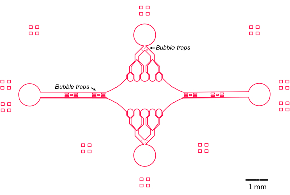
Figure 2: Schematic of the microfluidic device design. Rectangular markings on the periphery are for visual aid in seeing the periphery of the channels. Please click here to view a larger version of this figure.

The central, rectangular device chamber serves as the main imaging area where microtubule seeds are attached, and microtubule extensions are polymerized off of these seeds. The chamber is intersected by a flow channel on each side, with straight channels along the x-axis serving as an inlet and outlet to facilitate rapid exchange of the reaction solution. Microtubule inlet channel is also used to introduce microtubule seeds into the chamber, with laminar flow resulting in the seed binding to the glass surface along the direction of flow. In the perpendicular (y-axis) direction, the flow channels branch into smaller channels towards the chamber, similar to some of the previous designs^25,28,36,39. The branching geometry is particularly suitable for studying the mechanical properties of microtubules. Flowing a solution into the central chamber from a direction perpendicular to the orientation of the microtubule seeds allows for flow-induced bending forces at near-normal angles. Furthermore, the inclusion of branching geometry with many smaller flow channels facilitates a more homogeneous force application over a wide area of the central chamber, which is not achieved by a simple single-channel flow geometry. In this way, the branching motif, while seemingly more complicated, can reduce overall complexity in determining the force imparted to microtubules (Figure 3). This design also features multiple lines of symmetry, allowing for ease of use and the opportunity to evaluate bending from several directions (e.g., top vs. bottom).

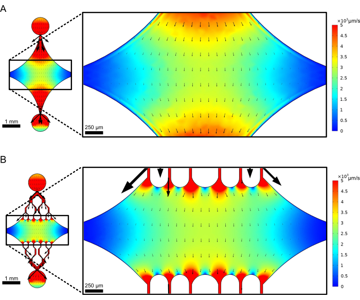
Figure 3: Inclusion of a branching motif results in a large area of similar flow. Simulations of two device designs under steady-state flow: one without branching channels (A) and one with branching channels (B). Arrows denote local flow direction and are proportional to flow magnitude. Surface coloration denotes centerline velocity. Images on the right show zoomed-in section of the device where microtubules (not shown) oriented along the x-axis would be subject to bending forces from a fluid flowing in the top port and out the bottom port. Incorporating branching channels increases the relative area subject to similar velocity fields while not increasing the volume of reagent required. This figure has been modified with permission from Rogers (2022)¹⁴. Please click here to view a larger version of this figure.

Notably, the device also implements a series of bubble traps in the inlet and outlet flow channels to prevent air bubbles from entering the central imaging chamber. Specifically, we chose to include arrays of micropillars within the flow path in order to block air bubbles from traveling past due to surface tension (Figure 2)⁴⁶. Furthermore, to prevent air entrainment, we designed the edges inside the device as smooth curves, as opposed to having oblique angles. Taken together, these design features reduce the possibility of air bubbles and increase the robustness of the device.

Microfluidic device fabrication
Determining the proper parameters for creating the device master required some optimization. As previously observed, this photoresist is very sensitive to key operating parameters such as ambient lighting and the rates of heating and cooling during the photolithography steps⁵⁰. For example, if the master was cooled too quickly after heating, thermal cracks could develop in the photoresist. This is undesirable, as the cracks can compromise channel integrity. While cracks could be resolved by re-heating the resist to a temperature near its transition temperature (~115 ˚C), we found that allowing the master to ambiently cool on the hot plate was the most robust way of preventing cracking. Furthermore, excess ambient light can result in unintended exposure of the photoresist, weakening the resist and resulting in the device features themselves (which should remain on the wafer after development) undergoing partial stripping away during the development step. For this reason, we encourage the development step to be performed the day after the post-exposure baking and ambient overnight cooling steps. Moreover, whenever the device master is not in use, we recommend storing it in a dark area or wrapped in aluminum foil to prevent degradation over time. Once these parameters were determined, the photolithography process was highly repeatable (Figure 4).

After the master was created, liquid PDMS was cast on top of the master, allowing the PDMS to cure and create a negative imprint of the master's features. We found that casting the PDMS at a thickness of 2-3 mm allowed for easy manipulation of the devices; in contrast, if spin-coated to achieve a thickness in the µm range, the PDMS was prone to tearing or self-adhering, making manipulation difficult. Furthermore, a thicker PDMS layer allows for easier plugging in of tubing, as the tubing will remain in the inlet/outlet ports without the need for a sealant or clamp.

Finally, while traditional flow-cell assays for these biological applications often use glass coverslips that have been pre-cleaned using a Piranha solution (hydrogen peroxide and sulfuric acid) and then silanized, we found that coverslips treated with an extended plasma clean and IPA wash were suitable for our purposes⁴⁷. Other applications, such as single-molecule imaging, may require a more extensive cover glass treatment.

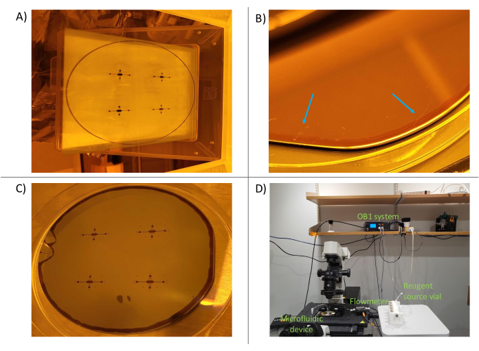
Figure 4: Photolithography process. (A) The mask with the desired design (mask made from chromium etched on glass). (B) Slight cracking of photoresist on the silicon wafer due to thermal stress (arrows highlight a few cracks). These cracks often stretch across the entire wafer. (C) The developed master. (D) The microfluidic setup on the microscope. Individual components are labeled in green. Please click here to view a larger version of this figure.

Microtubule growth, stabilization, and bending
GMPCPP-grown microtubule seeds serve as nucleation sites for microtubule extensions to polymerize and are themselves stable against depolymerization for several hours at room temperature. The seeds were bound to the glass coverslip in the microfluidic channel using an anti-rhodamine antibody⁴⁷. Dynamic microtubule extensions were then grown in the presence of soluble tubulin (fluorescently labeled but not rhodamine-conjugated) and GTP. In this way, the seed nucleation sites were attached to the glass coverslip, but the extensions were not. During the 15-min extension growth period, microtubule extensions polymerized and depolymerized stochastically, as expected due to their intrinsic dynamic instability⁴⁹. Following this growth period, a 10 µM Taxol washout was carried out to eliminate any remaining tubulin from the solution and stabilize the microtubule extensions that had formed. The stabilization is key, as the microtubule extensions would otherwise depolymerize upon tubulin depletion. In addition to binding and stabilizing microtubule polymer, Taxol has also been demonstrated to impact microtubule polymer mechanics and may induce curvature in the otherwise linear microtubule extensions^51,52,53,54. The results shown here reflected these observations; however, the curling of the microtubule extensions is undesirable, as this results in uneven forces imparted along the lattice during bending. Therefore, only microtubules that remained relatively straight after stabilization were used for bending analysis. Alternatively, after the initial growth period, a secondary growth period with a solution of tubulin and GMPCPP (as opposed to the initial GTP) can be used to create stable 'caps' on the growing ends of the microtubule lattice and prevent depolymerization⁵⁵.

Microtubules were then bent by flowing in the buffer solution using the pressure control system to maintain a constant upstream pressure (Figure 5, Supplementary Video 1). In this way, we could approximate the local flow experienced by the microtubules. By flowing fluid in from the top and out of the bottom device port, the orientation of the flow was intended to be perpendicular to the seeding orientation.

Figure 5: The microfluidic setup can be used to bend stabilized microtubules. Microtubules in a resting state after stabilization with paclitaxel are bent during pulsatile flow. A constant upstream pressure of 30 mbar drives flow (arrow denotes direction of flow). Please click here to view a larger version of this figure.

Determination of flow profile in the microfluidic device
The centerline velocity in the microfluidic can be computationally simulated using COMSOL software (simulation software, Figure 6A). However, the microtubules are attached to the glass coverslip for TIRF microscopy within ~100 nm of the surface. Therefore, the velocity experienced by the microtubule is not the same as that predicted in the 2D simulation. To approximate the local flow experienced by the microtubules, we used the general Navier-Stokes equation for an incompressible fluid flow in one dimension:

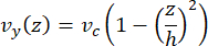
Here, z is the height of the microtubules in the device, h is the overall height of the device, and v_c is the centerline velocity in the device. By definition of the system, the z-origin is the center of the device (Figure 6B). Using this definition and a channel height of 13 µm, the height of the microtubules is approximated as z = -6.4 µm. Solving this equation yields an estimate for the local fluid velocity experienced by the microtubules:

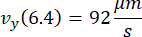
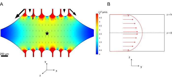
Figure 6: Defining the system for fluid flow analysis of fluid entering the device at the top port and exiting at the bottom port (ports not shown). (A) Simulation of scaled centerline velocity field as in Figure 3B. Star denotes the area of interest for panel B. (B) Cross-sectional representation of the device. Fully developed fluid flow profile is in the y-direction with a centerline velocity v_c at z = 0 and a no-slip boundary condition at the walls. Note that the arrows in this panel are not to scale with respect to the actual velocity field shown in panel A. This figure has been modified with permission from Rogers (2022)¹⁴. Please click here to view a larger version of this figure.

Beyond simulations, fluid velocity can be controlled using a flow controller based on a volumetric flow rate rather than maintaining pressure. Furthermore, the local flow rate in each device can be directly determined by including fluorescent beads and monitoring their velocity, thus alleviating any sample-to-sample variability.

Computational modeling and gradient demonstrations
Finally, we performed computational simulations in combination with experiments to demonstrate the feasibility of using this device for high-throughput experiments. Along with the ability to bend microtubules in multiple directions thanks to the device's symmetry, the simulations showed that the device can maintain precise gradients, enabling the simultaneous investigation of multiple experimental conditions (Figure 7A). Preliminary experiments (methods not explicitly stated as part of this publication) using fluorescent dye in solution demonstrated consistency with the computational predictions (Figure 7B). Furthermore, we successfully demonstrated the partitioning of different proteins in different areas of the device by simultaneously growing microtubule extensions with different fluorescent labels (Figure 8). To our knowledge, this is the first application of high-throughput microfluidics to microtubule investigations. This feature of this device can be used to reduce the time and quantities of needed reagents while also improving experimental robustness. For example, the effects of different proteins or distinct concentrations of individual proteins on microtubule mechanics and dynamics can be simultaneously investigated simultaneously in a single device.

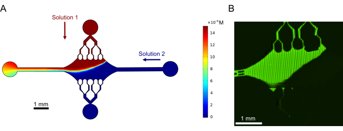
Figure 7: Gradient formation. (A) Simulation of a gradient of two solutions entering the device at the same inlet pressure (50 mbar) and concentration (15 µM). Inlet ports for each solution are denoted with colored arrows (one solution in the top port and another solution in the right port), and the two remaining ports serve as outlets. Heatmap shows the concentration profile of the top solution. Steady state was achieved at t = 5 s. (B) Experimental generation of a similar gradient using fluorescent dye in solution in the top port and buffer in the right port. Image is a raster layer made by stitching each field of view (80 µm × 80 µm) to resolve the entire device area. This figure has been modified with permission from Rogers (2022)¹⁴. Please click here to view a larger version of this figure.

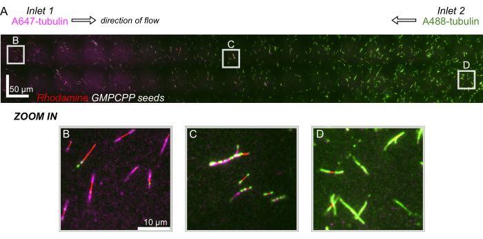
Figure 8: Demonstrating a protein gradient in the microfluidic device. AlexaFluor647 labeled tubulin (magenta) was flown in inlet 1, and AlexaFluor488 labeled tubulin (green) was flown in inlet 2 of the device at equal concentrations and flow rates. Flow was oscillated on/off in 90 s increments to allow for tubulin polymerization from stabilized-GMPCPP seeds (red) while inhibiting mixing. (A) Large-scale raster layer made by stitching fields of view (80x80 µm) to resolve the entire length of the device. Letters designate the relative location of individual fields of view in subsequent panels. Scale bar is 50 µm in X and Y-position. (B) Field of view near inlet 1 of the device, where extensions are comprised predominately of A647-labeled tubulin. (C) Field of view near the middle of the device, where extensions are comprised of a mixture of labeled tubulins, as predicted. (D) Field of view near the bottom of the device, where extensions are comprised predominately of A488-labeled tubulin. Please click here to view a larger version of this figure.

A process flow diagram (PFD) for the microfluidics experimental setup on a microscope is shown in Supplementary Figure 1.

Supplementary Figure 1: A process flow diagram (PFD) for the microfluidics experimental setup on a microscope. Please click here to download this File.

Supplementary Video 1. The microfluidic setup can be used to bend stabilized microtubules. Microtubules in a resting state after stabilization with paclitaxel are bent during pulsatile flow. A constant upstream pressure of 30 mbar drives flow. Video playback rate 10 fps. Please click here to download this File.

Supplementary File 1: A CAD file of the microfluidic mask design. Please click here to download this File.

Discussion

The primary goal of this protocol was to design and fabricate a microfluidic device suitable for the investigation of microtubule mechanics in vitro. The design was based on the desire to utilize the intrinsic benefits of PDMS-based microfluidic devices while also including a combination of features that would enable robust and customizable high-throughput experimentation.

This goal has been successfully achieved, resulting in fabrication protocols and general guidelines that can serve as a basis for future users of this system. The inclusion of redundant bubble traps in the device decreases the likelihood of protein denaturation due to the presence of air bubbles. While we still have some unplugging and re-plugging of tubing in the device, these bubble traps reduce the probability of experimental failure. Future improvements to the microfluidic setup could even further reduce the amount of manual tubing manipulations made during an experiment. Moreover, the integration of the microfluidic device with an automated flow control software allows for a significant customization of experimental conditions while reducing the possibility of manual error. We have demonstrated the device's successful performance by fabricating the device and then growing, stabilizing, and bending microtubule extensions in the device using automatic, controller-regulated flow. Furthermore, by establishing a gradient of distinct fluorescently labeled tubulin solutions within the same device, we showed that multiple conditions can be run simultaneously in a single device. Aided by computational modeling and analysis techniques, our system can probe and determine the biomechanical properties of microtubules, such as flexural rigidity^{52,56,57,58,59}.

Potential future improvements would facilitate an even more robust system and associated experimental analysis. First, the photoresist deposition, exposure, and baking were crucial parameters that demonstrated some variability. The relatively tall feature sizes of the SPR photoresist required very gradual heating and cooling to prevent thermal cracking, which could ruin the devices. While thinner devices were attempted, we found issues with the manipulation of these smaller feature sizes. Attention to detail and patience are crucial for replicating devices of this thickness with SPR photoresist. Different photoresists may be used to solve this issue, depending on availability.

Taken together, the microfluidic device and protocol here allow for a range of experimental setups with more robust, high-throughput testing capabilities than previous flow-cell assays⁴⁷. Furthermore, experiments can be automated using flow controllers to maintain precise flow profiles or concentration gradients in the device, reducing variability inherent to manual users. Future potential applications of this setup include investigating the effects of microtubule-associated proteins on microtubule flexural rigidity, dynamics, lattice damage, and repair, as well as the biomechanical interactions of microtubules and actin filaments^{54,60,61,62,63,64,65,66,67,68,69,70}. The integration of microfabrication, automated flow control, and computational modeling and analysis techniques creates a versatile system suited for studying the cellular cytoskeleton in vitro.

Materials

List of materials used in this article

Name	Company	Catalog Number	Comments
0.6 mL microcentrifuge tubes (clear)	Any brand		Low retention type is preferred
1.5 mL microcentrifuge tubes (clear)	Any brand		Low retention type is preferred
1.5 mm standard biopsy punch	Integra LifeSciences	33-31A-P/25
100x/1.49 numerical aperture TIRF objective	Nikon
22 x 22 mm glass coverslips	ThorLabs	CG15CH
3" single side polished silicon wafers	University Wafer	447
4" Petri dish	Any brand
450 µL, Open-Top Thinwall Ultra-Clear Tube	Beckman Coulter, Inc.	345843	Referred to as 'airfuge tube' in the protocol
488-, 561, and 640-nm solid state lasers	Nikon
A-95 Fixed-Angle Rotor	Beckman Coulter, Inc.	347595
Acetone	Any brand
Airfuge Air-Driven Ultracentrifuge	Beckman Coulter, Inc.	347854	Referred to as 'airfuge' in the protocol
Alexa Fluor 488 Microscale Protein Labeling Kit	Thermo Fisher Scientific	A30006
Aluminum foil	Any brand
Andor iXon Ultra EM-CCD	Nikon
Andor NEO sCMOS	Nikon
AutoCAD	Autodesk		Generic versions can be used
Bovine brain unlabeled tubulin (purified)	N/A		Made in house, but can be purchased
Casein	MilliporeSigma	C7078
Catalase	MilliporeSigma	C9322
Clean Dry Air (CDA) (pressurized gas)	Any brand
Compressed air supply	Any brand		Connects to the microfluidic flow controller
COMSOL Multiphysics software	COMSOL, Inc.
Custom brass stage adapter	N/A		Made in house to fit our 22 mm x 22 mm coverslips onto the microscope
De-ionized water	Any brand
Dessicator	Any brand
D-glucose	MilliporeSigma	G7528
Dithiothreitol (DTT)	MilliporeSigma	D0632
EGTA	MilliporeSigma	324626
Elveflow Smart Interface (ESI) software	Elveflow
Flangeless PFA fittings with ETFE ¼”-28 to 1/16” outer diameter ferrules	Darwin Microfluidics	CIL-XP-245X	Used to connect the tubing from the micrewtube source vials to the flow sensor via the pressurized reservoir rack
Fluiwell 4-Channel 2 mL Low Pressure	Fluigent	14002001	Used to connect the flow control system to the the micrewtubes. Also refered to as 'pressurized reservoir rack'
Fume hood	Any brand
Glucose oxidase	MilliporeSigma	G6125
GMPCPP	Jena Bioscience	NU-405L
Guanosine triphosphate (GTP)	MilliporeSigma	G8877
Hot plate	Any brand
HS-625 high-speed emission filter wheel	Finger Lakes Instrumentation
ImageJ software	N/A		Open access
Incubator	Any brand
Isopropyl alcohol	Any brand
Karl Suss MA-6 mask aligner	SUSS MicroTec
Magnesium chloride	MilliporeSigma	1.05833
MATLAB software	MathWorks
MEGAPOSIT SPR 220 7.0 photoresist	Dow, Inc.
Microfluidic Fittings 6-40 to 1/4"-28 Adapters Kit	Darwin Microfluidics	LVF-KFI-08	Used to connect the tubing from the micrewtube source vials to the flow sensor via the pressurized reservoir rack (Fluiwell rack)
Microfluidic Fittings Female Luer Lock Adapter Kit	Darwin Microfluidics	LVF-KFI-04	Used to connect the syringe to the tubing
Microfluidic flow controller	Elveflow	OB1 MK3+
Microfluidic flow sensor	Elveflow	MFS3	This flow sensor range is 0-80 μL
MICROPOSIT MF-319 developer	Dow, Inc.
Microscope	Nikon	Eclipse Ti
NIS-Elements software	Nikon
Nitrogen (pressurized gas)	Any brand
Objective heater	Tokai Hit
One-Piece Fingertight 10-32 Coned Fitting for 1/16" OD Tubing	Darwin Microfluidics	CIL-F-120X	Used to connect the syringe to the tubing
Paclitaxol (Taxol)	Tocris Bioscience	1097
Photolithography masks	N/A		Made by an external party using our designs
PIPES	Thermo Fisher Scientific	172615000
Plasma cleaner	Harrick Plasma	PDC-32G
Plasma flowmeter system	Harrick Plasma	PDC-FMG	Integrates with plasma cleaner to enable flow control of pressurized gas
Plastic bulb pipet	Any brand
Pluoronic F-127	MilliporeSigma	P2443	Referred to as 'poloxomer 407' in the protocol
Potassium chloride	Research Products International	P41000
Saint Gobain Performance Plastics Tube Tygon .020 ID	Thermo Fisher Scientific	50-206-8921	Refered to as '1.5 mm tubing' and 'tubing' in the protocol
Scalpel	Any brand
Spin coater	Cost Effective Equipment, LLC.	200x	This model may be discontinued
Standard pipets and tip sets	Any brand
Standard plastic syringe	Any brand		We used a 10 mL Luer-slip syringe
Sylgard 184 silicone elastomer kit	Dow, Inc.		Referred to as 'PDMS' and 'curing agent' in the protocol
T339 Micrewtube with Lip Seal and Flat Screw Cap	Medline Industried, LP.	T339	Referred to as 'source vial' in the protocol. We used both 0.5 mL and 1.5 mL sizes
TAMRA, SE; 5-(and-6)-Carboxytetramethylrhodamine, Succinimidyl Ester	Invitrogen	C1171	Referred to as 'TTR' in the protocol
Trichloro(1H, 1H, 2H, 2H-perfluorooctyl) silane	MilliporeSigma	448931
Trion Phantom RIE ICP	Trion Technology, Inc.		This plasma cleaner is only used in Step 1.1 of the protocol. Another plasma cleaner, like the one used for PDMS bonding, can be used instead; we just prefer the much lower vacuum achievable by this system for cleaning the silicon wafer
TRITC Polyclonal Antibody	Thermo Fisher Scientific	A6397	Referred to as 'anti-rhodamine antibody' in the protocol
Tweezers	Any brand
Vacuum pump	Any brand

References

- Whitesides, G. M. The origins and the future of microfluidics. Nature. 442, 368-373 (2006).
- Whitesides, G. M., Stroock, A. D. Flexible methods for microfluidics. Phys Today. 54 (6), 42(2001).
- Squires, T. M., Quake, S. R. Microfluidics: Fluid physics at the nanoliter scale. Rev Mod Phys. 77, 977(2005).
- Beebe, D. J., Mensing, G. A., Walker, G. M. Physics and applications of microfluidics in biology. Annu Rev Biomed Eng. 4, 261-286 (2002).
- Ng, J. M. K., Stroock, A. D., Whitesides, G. M. Components for integrated poly(dimethylsiloxane) microfluidic systems. Electrophoresis. 23 (20), 3461-3473 (2010).
- Dellaquila, A. Five Short Stories on The History of Microfluidics. , https://www.elveflow.com/microfluidic-reviews/general-microfluidics/history-of-microfluidics/ (2025).
- Duffy, D. C., McDonald, J. C., Schueller, O. J. A., Whitesides, G. M. Rapid prototyping of microfluidic systems in poly(dimethylsiloxane). Anal Chem. 70 (23), 4974-4984 (1998).
- Dittrich, P. S., Manz, A. Lab-on-a-chip: Microfluidics in drug discovery. Nat Rev Drug Discov. 5 (3), 210-218 (2006).
- Neužil, P., Giselbrecht, S., Länge, K., Huang, T. J., Manz, A. Revisiting lab-on-a-chip technology for drug discovery. Nat Rev Drug Discov. 11 (8), 620-632 (2012).
- Manz, A., Graber, N., Widmer, H. M. Miniaturized total chemical analysis systems: a novel concept for chemical sensing. Sens Actuators B: Chem. 1 (1-6), 244-248 (1990).
- Harrison, D. J., et al. Micromachining a miniaturized capillary electrophoresis-based chemical analysis system on a chip. Science. 261 (5123), 895-897 (1993).
- Knight, J. Microfluidics: Honey, I shrunk the lab. Nature. 418 (6897), 474-475 (2002).
- Photolithographic fabrication techniques for transistors which are an integral part of a printed circuit. Nall, J. R., Lathrop, J. W. 1957 International Electron Devices Meeting, Washington, DC, USA, , (1957).
- Rogers, M. The design and fabrication of a two-layer microfluidic device for studying microtubules in vitro [Master's Thesis]. , Vanderbilt University. Nashville, TN. (2022).
- Lee, J. B., Choi, K. H., Yoo, K. Innovative SU-8 lithography techniques and their applications. Micromachines. 6 (1), 1-18 (2015).
- Kim, P., et al. Soft lithography for microfluidics: A Review. Biochip J. 2 (1), 1-11 (2008).
- Venkatesan, S. u, Jerald, J., Asokan, P., Prabakaran, R. A Comprehensive Review on Microfluidics Technology and its Applications. Recent Advances in Mechanical Engineering. , Springer. Singapore. 235-245 (2020).
- Minteer, S. Microfluidic Techniques: Reviews and Protocols. , Humana Press. New Jersey. (2006).
- Mitra, S. K., Chakraborty, S. Microfluidics and Nanofluidics Handbook: Fabrication, Implementation, and Applications. , Taylor and Francis Group. Florida. (2016).
- Alberts, B., et al. Molecular Biology of the Cell. , Garland Science. New York. (2014).
- Howard, J. Mechanics of Motor Proteins and the Cytoskeleton. , Springer. Heidelberg. (2001).
- Hawkins, T., Mirigian, M., Selcuk Yasar, M., Ross, J. L. Mechanics of microtubules. J Biomech. 43 (1), 23-30 (2010).
- Gardel, M. L., Kasza, K. E., Brangwynne, C. P., Liu, J., Weitz, D. A. Chapter 19: Mechanical Response of Cytoskeletal Networks. Methods Cell Biol. 89, 487-519 (2008).
- Caporizzo, M. A., Prosser, B. L. The microtubule cytoskeleton in cardiac mechanics and heart failure. Nat Rev Cardiol. 19 (6), 364-378 (2022).
- Schaedel, L., et al. Microtubules self-repair in response to mechanical stress. Nat Mater. 14 (11), 1156-1163 (2015).
- Chu, S. H., et al. A microfluidic device for in situ fixation and super-resolved mechanosensation studies of primary cilia. Biomicrofluidics. 13 (1), 014105(2019).
- Geisterfer, Z. M., Zhu, D. Y., Mitchison, T. J., Oakey, J., Gatlin, J. C. Microtubule growth rates are sensitive to global and local changes in microtubule plus-end density. Curr Biol. 30 (15), 3016-3023 (2020).
- Schaedel, L., et al. Lattice defects induce microtubule self-renewal. Nat Phys. 15 (8), 830-838 (2019).
- Aher, A., et al. CLASP mediates microtubule repair by restricting lattice damage and regulating tubulin incorporation. Curr Biol. 30 (11), 2175-2183 (2020).
- Duellberg, C., Cade, N. I., Holmes, D., Surrey, T. The size of the EB cap determines instantaneous microtubule stability. ELife. 5, e13470(2016).
- Fourniol, F. J., et al. Micropattern-guided assembly of overlapping pairs of dynamic microtubules. Methods Enzymol. 540, 339-360 (2014).
- Vleugel, M., Roth, S., Groenendijk, C. F., Dogterom, M. Reconstitution of basic mitotic spindles in spherical emulsion droplets. J Vis Exp. (114), e54278(2016).
- Duellberg, C., Cade, N. I., Surrey, T. Microtubule aging probed by microfluidics-assisted tubulin washout. Mol Biol Cell. 27 (22), 3563-3573 (2016).
- VanDelinder, V., Brener, S., Bachand, G. D. Mechanisms underlying the active self-assembly of microtubule rings and spools. Biomacromolecules. 17 (3), 1048-1056 (2016).
- Roth, S., Gârlea, I. C., Vleugel, M., Mulder, B. M., Dogterom, M. Reconstitution of basic mitotic spindles in cell-like confinement. bioRxiv. , (2019).
- Xu, Z., et al. Microtubules acquire resistance from mechanical breakage through intralumenal acetylation. Science. 356 (6335), 328-332 (2017).
- Fanalista, F., et al. Shape and size control of artificial cells for bottom-up biology. ACS Nano. 13 (5), 5439-5450 (2019).
- Velve-Casquillas, G., Costa, J., Carlier-Grynkorn, F., Mayeux, A., Tran, P. T. A fast microfluidic temperature control device for studying microtubule dynamics in fission yeast. Methods Cell Biol. 97, 185-201 (2010).
- Portran, D., Schaedel, L., Xu, Z., Théry, M., Nachury, M. V. Tubulin acetylation protects long-lived microtubules against mechanical ageing. Nat Cell Biol. 19 (4), 391-398 (2017).
- Huang, Y. M., Uppalapati, M., Hancock, W. O., Jackson, T. N. Microtubule transport, concentration and alignment in enclosed microfluidic channels. Biomed Microdevices. 9 (2), 175-184 (2007).
- Uppalapati, M., Huang, Y., Shastry, S., Jackson, T. N., Hancock, W. O. Microtubule Motors in Microfluidics. Methods in Bioengineering: Microfabrication and Microfluidics. , Artech House Publishers. Boston, MA. (2009).
- Sung, J. H., Shuler, M. L. Prevention of air bubble formation in a microfluidic perfusion cell culture system using a microscale bubble trap. Biomed Microdevices. 11 (4), 731-738 (2009).
- Williams, M. J., et al. A low-cost, rapidly integrated debubbler (RID) module for microfluidic cell culture applications. Micromachines. 10 (6), 360(2019).
- Nakayama, T., et al. Circumventing air bubbles in microfluidic systems and quantitative continuous-flow PCR applications. Anal Bioanal Chem. 386 (5), 1327-1333 (2006).
- Park, S., Cho, H., Kim, J., Han, K. -H. Lateral degassing method for disposable film-chip microfluidic devices. Membranes. 11 (5), 316(2021).
- Pereiro, I., Fomitcheva Khartchenko, A., Petrini, L., Kaigala, G. V. Nip the bubble in the bud: A guide to avoid gas nucleation in microfluidics. Lab Chip. 19 (14), 2296-2314 (2019).
- Gell, C., et al. Microtubule dynamics reconstituted in vitro and imaged by single-molecule fluorescence microscopy. Methods in Cell Biol. 95, 221-245 (2010).
- Hyman, A. A., Salser, S., Drechsel, D. N., Unwin, N., Mitchison, T. J. Role of GTP hydrolysis in microtubule dynamics: Information from a slowly hydrolyzable analogue, GMPCPP. Mol Biol Cell. 3 (10), 1155-1167 (1992).
- Mitchison, T., Kirschner, M. Dynamic instability of microtubule growth. Nature. 312 (5991), 237-242 (1984).
- Bartlett, N. W., Wood, R. J. Comparative analysis of fabrication methods for achieving rounded microchannels in PDMS. J Micromech Microeng. 26 (11), 115013(2016).
- Yang, C. P. H., Horwitz, S. B. Taxol®: The first microtubule stabilizing agent. Int J Mol Sci. 18 (8), 1733(2017).
- Gittes, F., Mickey, B., Nettleton, J., Howard, J. Flexural rigidity of microtubules and actin filaments measured from thermal fluctuations in shape. J Cell Biol. 120 (4), 923-934 (1993).
- VanBuren, V., Cassimeris, L., Odde, D. J. Mechanochemical model of microtubule structure and self-assembly kinetics. Biophys J. 89 (5), 2911-2926 (2005).
- Dye, R. B., Fink, S. P., Williams, R. C. Taxol-induced flexibility of microtubules and its reversal by MAP-2 and Tau. J Biol Chem. 268 (10), 6847-6850 (1993).
- Drechsel, D. N., Kirschnert, M. W. The minimum GTP cap required to stabilize microtubules. Curr Biol. 4 (12), 1053-1061 (1994).
- Wisanpitayakorn, P., Mickolajczyk, K. J., Hancock, W. O., Vidali, L., Tüzel, E. Measurement of the persistence length of cytoskeletal filaments using curvature distributions. Biophys J. 121 (10), 1813-1822 (2022).
- Mickey, B., Howard, J. Rigidity of microtubules is increased by stabilizing agents. J Cell Biol. 130 (4), 909-917 (1995).
- Brangwynne, C. P., et al. Bending dynamics of fluctuating biopolymers probed by automated high-resolution filament tracking. Biophys J. 93 (1), 346-359 (2007).
- Venier, P., Maggs, A. C., Carlier, M. F., Pantaloni, D. Analysis of microtubule rigidity using hydrodynamic flow and thermal fluctuations. J Biol Chem. 269 (18), 13353-13360 (1994).
- Felgner, H., Frank, R., Schliwa, M. Flexural rigidity of microtubules measured with the use of optical tweezers. J Cell Sci. 109 (Pt 2), 509-516 (1996).
- Felgner, H., et al. Domains of neuronal microtubule-associated proteins and flexural rigidity of microtubules. J Cell Biol. 138 (5), 1067-1075 (1997).
- Nishida, K., et al. Effects of three microtubule-associated proteins (MAP2, MAP4, and Tau) on microtubules' physical properties and neurite morphology. Sci Rep. 13, 8870(2023).
- Akhmanova, A., Steinmetz, M. O. Control of microtubule organization and dynamics: two ends in the limelight. Nat Rev Mol Cell Biol. 16 (12), 711-726 (2015).
- Brouhard, G. J., Rice, L. M. Microtubule dynamics: An interplay of biochemistry and mechanics. Nat Rev Mol Cell Biol. 19 (7), 451-463 (2018).
- Lawrence, E. J., Chatterjee, S., Zanic, M. More is different: Reconstituting complexity in microtubule regulation. J Biol Chem. 299 (12), 105398(2023).
- Howard, J., Hyman, A. A. Dynamics and mechanics of the microtubule plus end. Nature. 422 (6933), 753-758 (2003).
- Mehidi, A., Aumeier, C. Regulation of the microtubule network; the shaft matters. Curr Opin Syst Biol. 34, 100457(2023).
- Verhey, K. J., Ohi, R. Causes, costs and consequences of kinesin motors communicating through the microtubule lattice. J Cell Sci. 136 (5), jcs260735(2023).
- Dogterom, M., Koenderink, G. H. Actin-microtubule crosstalk in cell biology. Nat Rev Mol Cell Biol. 20 (1), 38-54 (2019).
- Théry, M., Blanchoin, L. Microtubule self-repair. Curr Opin Cell Biol. 68, 144-154 (2021).
Reprints and Permissions