Efficient Multiscale Gradient-Domain Filtering for Image and Video Dehazing with Enhanced Temporal Coherence

Summary

The protocol here integrates Minimum-Preserving Subsampling with Gradient-Domain Weighted Guided Filtering to enhance the real-time dehazing capabilities of the light scattering model. Averaging the RGB values from the source image's top 0.1% brightest pixels in the dark channel produces atmospheric light, and the gradient-based Correlation Factor is used for video processing consistency.

Abstract

Dehazing is crucial in computer vision to restore image clarity affected by atmospheric scattering. Existing methods suffer from high computational costs, loss of gradient details, and flickering artifacts in video applications. To enhance efficiency and visual quality, this work proposes a multiscale gradient-domain weighted guided image filter-based dehazing technique applicable to both videos and images. To estimate atmospheric parameters and reduce computational complexity, Minimum Preserving Subsampling (MPS) has been employed. Next, an iterative up-sampling process with the Gradient-domain Weighted Guided Image Filter (GWGIF) refines the transmission map, preserving a significant amount of gradient features and thereby enhancing texture and edge retention. For video dehazing, the Gradient-Based Correlation Factor (GCF) is introduced, resulting in a significant reduction in flickering artifacts compared to existing methods. Experimental evaluations demonstrate the superiority of our approach, achieving a Perception-based Image Quality Evaluator (PIQE) score of 26.98, a Natural Image Quality Evaluator (NIQE) score of 2.78, and a Blind/Referenceless Image Spatial Quality Evaluator (BRISQE) score of 20.18, reflecting improved perceptual quality. Furthermore, the proposed method ensures high temporal coherence in video dehazing, with Mean Square Error (MSE) deviation of 0.003, making it ideal for real-time applications such as autonomous vehicles, surveillance, and remote sensing.

Introduction

Haze is an atmospheric phenomenon that makes it more difficult to see distant objects when light is scattered by smoke, water droplets, or dust particles. Image deterioration due to haze is detrimental to computer vision applications^1,2,including video analysis, autonomous vehicles, and surveillance. To improve the performance of computer vision, as a first step in processing, a dehazing strategy is essential for removing haze components from images. The term "dehazing" refers to the steps used to restore clarity to a blurry or otherwise unusable image. In recent years, several techniques have been developed for image dehazing. The dehazing problem represents the target (hazy) image I^hazy(x) of the color channel at location x as shown in (1) as taken from He et al.³.

    1

J^clear(x) represents the transparent image, whereas L_atm and t_map represent the global atmospheric light and the medium transmission map, respectively. The portion of the light that is picked up by the camera sensors is denoted by the t_map distance d(x) as calculated by the distance between the scene and the camera in He et al.³as shown in (2).

    2

Here, β represents the transmission coefficient for air scattering.

Recovering J^clear(x) from I^hazy(x) during the dehazing process, it is shown in (3), which is achieved after rearrangement of (1). Here, t represents the atmosphere's light transmittance, also known as the transmission coefficient.

    3

The dark channel prior (DCP)³ model is among the most well-known atmospheric models for this purpose. Among the well-known physical model-based dehazing techniques, DCP is the most widely used, which assumes that at least one color channel contains pixels with extremely low intensities in a haze-free image. This prior is used to estimate the transmission map using DCP and recover the scene radiancefrom (1). However, this technique is time-consuming and over-saturates the sky region in the Image.

The motivation for this research stems from the need to enhance visibility in computer vision applications where haze significantly degrades image quality. The approach not only accelerates the dehazing process but also ensures that image details, such as edges and textures, are preserved. Moreover, the research extends its dehazing algorithm to videos, tackling a critical issue in video processing. Sometimes, under different lighting conditions, the visibility of images changes, which presents another challenge in many applications, such as autonomous driving and surveillance.

Validation of the proposed dehazing algorithm was performed through extensive experiments on various publicly available Image and video datasets. The datasets comprise both synthetic and real-world hazy scenes, allowing for a comprehensive evaluation under diverse conditions. Experimental validation across diverse real-world video sequences (Riverside, Crossroad, Haze road, Ship)⁴ and static images⁵ with varying haze densities, evaluated using established metrics (FADE, NIQE, PIQE, BRISQUE)⁶ and compared against nine state-of-the-art methods, demonstrates the algorithm's practical applicability for automotive, surveillance, maritime, and mobile computing domains while maintaining real-time performance. Performance was assessed using subjective visual comparisons and objective quality metrics, demonstrating competitiveness with state-of-the-art approaches in terms of accuracy and computational efficiency.

The proposed work is designed for real-time performance and has been tested on images and videos with resolutions up to 1920 × 1080 pixels. To ensure efficient processing, all experiments have been conducted on a workstation equipped with an Intel i3-6006U CPU (2.00 GHz) and 12 GB of RAM. While the method demonstrates strong performance across various real-world scenarios, it may exhibit reduced accuracy under extremely dense haze conditions where transmission estimation becomes unreliable. These details highlight the practicality and limitations of the proposed approach in real-world deployment.

To overcome various challenges, this research proposes a novel approach using a multiscale GWGIF for dehazing images and videos. By integrating an MPS method, the study introduces a computationally efficient technique for estimating the transmission map, which is a key factor in dehazing. Flickering artifacts have been addressed by incorporating a novel GCF method that maintains temporal coherence between consecutive frames, ensuring both computational efficiency and high-quality results. This study contributes to the development of more robust image and video enhancement techniques. Figure 1 illustrates the transmission map calculated using the MPS method, and Figure 2 shows the proposed method combining MPS and GCF. The novelty of our work lies in the development of a real-time image and video dehazing algorithm based on multiscaling with a gradient-based weighted guided filter, which addresses the computational bottlenecks of traditional dehazing methods. Specifically, our main novel contributions are: (1) the MPS technique that retains critical dark regions for accurate transmission estimation while reducing computational load; (2) GWGIF that specifically preserves firm edges during transmission map refinement; (3) Optimized atmospheric light estimation that focuses only on the top 0.1% brightest pixels; (4) GCF for video dehazing that measures frame similarity through gradient information; (5) A temporal optimization system that reuses calculations between similar video frames to achieve real-time processing.

This method achieves real-time performance while delivering dehazing quality comparable to, or better than, that of state-of-the-art algorithms, as demonstrated by extensive experiments presented in the article [Figure 3, Figure 4, Figure 5, Figure 6, and Figure 7].

Protocol

This work used synthetic or natural scene images with no human subjects involved. Therefore, no ethics approval was required.

This image dehazing protocol is developed on a standard computing setup and is designed to enhance the clarity and visibility of hazy images. The work environment is MATLAB⁷. The approach follows a systematic process involving haze estimation, refinement, and image restoration. By gradually improving image quality while preserving important details, the method delivers clear and visually appealing results. It has been tested on widely used datasets⁸ and evaluated using standard image quality measures, demonstrating its effectiveness and suitability for academic or research-based applications. Important explanations and equations for the protocol, materials, and equipment, as well as the steps of the proposed solution, have been provided in the sections below. Evaluation parameters have also been outlined.

1. Materials and equipment

The experiment is developed using MATLAB Online (24.2.0.2871072 (R2024b) Update 5) and executed on a system with an Intel i3-6006U CPU (2.00 GHz). The image datasets^5,8 used for the implementation are sourced from the referenced literature. The methodology includes the use of a 5 × 5 Gaussian filter with bilinear interpolation, transmission map estimation using the MPS algorithm⁹, and refinement through the GWGIF filter, all carried out on a suitable computing infrastructure. Details and links of all the materials and equipment used in the research are mentioned in Table of Materials.

2. Experimental setup

The experimental setup involves implementing the proposed image and video dehazing approach in a scientific computing environment that supports matrix-based image processing and visualization. Standard benchmark datasets^5,8, consisting of hazy images and videos¹⁰, as referenced in established literature, were used to evaluate the method's performance. The algorithm follows a multiscale processing framework, utilizing image pyramids and gradient-based correlation to guide the computation and refinement of the adaptive transmission map. For video sequences, frames are extracted at fixed intervals, and the GCF is used to determine whether to reuse or recompute the transmission map. The effectiveness of the dehazed outputs was assessed using widely recognized image quality metrics, including NIQE, PIQE, BRISQE, FADE, and MSE, ensuring both subjective and objective evaluation of the restoration quality.

3. Parameters used for evaluation

For objective evaluation, five quality metrics have been used: (1) FADE (Fog-Aware Density Evaluator)⁸; (2) NIQE (Natural Image Quality Evaluator)¹¹; (3) PIQE (Perception-based Image Quality Evaluator)¹²; (4) BRISQUE (Blind/Referenceless Image Spatial Quality Evaluator)¹³; (5) MSE (Mean Squared Error) between consecutive frames¹⁴.

4. Methodology of single-image and video dehazing

1. Convert and construct an image pyramid
   Single-image dehazing begins by converting the input color image to grayscale (). An image pyramid {, ...,, } is then constructed by recursively downsampling I^hazy with a factor of 2 until the coarsest level I_L is achieved, such that the maximum dimension is no larger than 320 pixels. This means L is determined by the requirement that max(W, H) <= 320, where W and H represent the width and height at the coarsest level L. The L value indicates the number of downsampling operations required to reach the desired coarsest level in the pyramid structure, as in Figure 2.
2. Estimation of transmission map
   The transmission map shows the percentage of light that is unscattered and reaches the camera's sensor. The transmission map accurately represents the picture's depth information, as it is a function of depth that is successive. The transmission map, t_map, is computed using ambient light to reconstruct a haze-free image J^clear (x). The primary objective of the study is to develop a computationally efficient transmission estimation method to expedite the dehazing process, as it was found that calculating a transmission map is the most time-consuming step. To be more specific, after estimating the transmission at a lower resolution and assuming that the transmission map is composed of constant parts, the results have been up-sampled, as depicted in Figure 2.
   1. Initial transmission map estimation using multiscale approach on MPS
      The initial transmission map, is obtained from the ImageImage , which has already been computed by downsampling the input hazy image at the coarsest level, L. Using the MPS approach⁹ on , the image is now divided into 5 × 5-sized square blocks, as shown in [Figure 1]. Further, is calculated by selecting the minimum value from each 5 × 5 block to obtain a down-sampled image, with dimensions (M/m) × (N/m) shown in ( 4) from Kansal et al.⁹. Here, min stands for the mathematical function to calculate the minimum intensity value in block BI_i.
      4
      the coarsest level dark channel image 4 is then obtained by applying a 3 × 3 minimum filter on as shown in ( 5) taken from Kansal et al. work⁹.
       5
      Where ω is a window of size 3 × 3. The initial transmission map is finally estimated using:
      6
      where w is a constant factor (typically 0).
      The MPS-based transmission map ensures improved contrast and detail recovery in regions severely impacted by haze by maintaining the local minimum values within the respective patches. However, the linear transformation²² based approach yields a transmission map that is more uniform (and less accurate) in removing haze, as it is unable to distinguish between regions with varying levels of haze intensity.
   2. Transmission refinement
      Since the initial transmission map () is estimated only at the coarsest level (L) of the image pyramid, it must be upsampled to match the original input image's resolution. Simple bilinear up-sampling B_Up(·) is applied to obtain a full-resolution transmission map. Moreover, to preserve the edge details in the transmission map, must be refined. Employing a guided filter and a gradient-guided filter, as applied in Van et al.¹⁴ and Kansal et al.⁹, would cause blurring artifacts in the transmission map, resulting in the loss of texture details and edge information, which would ultimately degrade dehazing performance. To address this issue, the gradient domain weighted guided image filtering (GWGIF)¹⁵ method has been employed to preserve image details effectively. Finally, the refined transmission is obtained as below from Wang et al.¹⁶.
       7
      GWGIF refines the initial transmission map by preserving edge structures and avoiding blurring artifacts typically introduced by standard guided filters. The following step has been followed to implement the GWGIF function¹⁷.
      Input:
      : Initial transmission map (low-resolution or coarse)
      : Original hazy image (used as guidance)
      Output:
      
      Step 1: Up sampled the initial transmission map
      Resized to match the size of I^hazy
      Step 2: Converted I^hazy to grayscale
      I^hazy = rgb2gray(I^hazy)
      Step 3: Applied the Gradient Domain Weighted Guided Filter as in (7)
      Obtained refined transmission map 
      The process computes the gradient magnitude from the guidance image using the Sobel operator, generates gradient-based weights, and integrates them into the guided filtering equation to enhance edge-aware smoothing. The output is a refined transmission map that significantly improves dehazing quality and detail preservation, as shown in Figure 4.
3. Atmospheric light estimation
   Global atmospheric light, in terms of model-based image dehazing, is essential. As stated by Zhang et al.¹⁸, brighter de-hazed images are produced by lower values of atmospheric light, while higher values of atmospheric light produce the darkest de-hazed images. The proposed work estimates atmospheric light from the dark channel image () obtained from the input hazy image. Then, the RGB values corresponding to the top 0.1% brightest pixels in the dark channel image are picked to obtain the final value of atmospheric light, as shown in ( 8) as given in, He et al.³. Here, γ represents the top 0.1 brightest pixels. These pixels typically correspond to the most haze-opaque regions in the image. From these selected pixels, their corresponding RGB values in the original Image are extracted and averaged to determine the global atmospheric light L_atm.
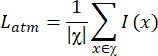    8
   Atmospheric light L_atm is calculated by selecting the top 0.1% brightest pixels from the dark channel image. This is performed as follows:
   Input:
   Hazy Image I^hazy RGB image)
   Output:
   Atmospheric light L_atm (a 3-element RGB vector)
   Steps:
   Step 1: Computed the Dark Channel of the Image:
   The dark channel image is .
   Step 2: Found Most Haze-Opaque Pixels
   Flattened the dark channel into a 1D array
   Sorted the pixel values in descending order.
   Selected the top 0.1% brightest pixels (i.e., highest values in dark channel → high haze concentration).
   Step 3: Picked Candidate Pixels in the Input Image
   Among the selected top 0.1% pixels (from the dark channel), identify the corresponding pixels in the original hazy image I^hazy.
   For each selected pixel, the intensity was computed (e.g., sum or norm of its RGB values).
   Step 4: Set Atmospheric Light L_atm
   The RGB value of the brightest pixel selected above has been taken as the estimated atmospheric light.
   The above procedure systematically estimates the atmospheric light, L_atm.
   The above procedure systematically estimates the atmospheric light L_atm by leveraging the dark channel prior to identifying the most haze-affected regions in the image. By excluding bright, clear areas and focusing on the top 0.1% darkest regions (indicative of dense haze), the method ensures a robust and accurate estimation of the global atmospheric light, which is a critical parameter for effective haze removal in single-image dehazing algorithms.
   1. Hazy image recovery
      Finally, after finding the atmospheric light L_atm and refined transmission map , the haze-free image J^clear(x) is obtained by using the Van et al.¹⁴, formulation in (9), which is given by
      9
      where γ is the transmission's lower bound (set to 0.05)
      As illustrated in Figure 1, the proposed transmission-map refinement method effectively preserves the complex characteristics of the picture and enables haze-free picture recovery.
4. Hazy video recovery
   The video dehazing approach presented in this work builds upon the single-image dehazing algorithm by incorporating temporal coherence considerations to prevent flickering artifacts. The authors recognize that applying single-image dehazing independently to each frame of a video would break temporal coherence between frames, resulting in visual inconsistencies. To address this issue, a novel video dehazing algorithm has been developed that quantifies temporal coherence between consecutive initial frames. This information is used to adaptively estimate transmission maps and atmospheric light values for the upcoming frames.
   1. Flickering artifacts
      The same image region may be captured at different pixel coordinates in consecutive frames of a video due to the movement of the object and/or camera. Flickering artifacts emerge as a result of these motions, which change the transmission values at the same spot. Motion estimation techniques, such as optical flow estimation¹⁹, can be used to track the location of a movable object and address these issues. However, motion estimation methods often need a high degree of computational complexity. Therefore, a simple probability model called a GCF has been used instead of explicitly computing the motions between frames. The differential image between the two consecutive frames serves as the foundation for this model.
   2. Gradient-based correlation factor
      The Gradient-Based Correlation Factor (GCF) measures the similarity between two consecutive video frames based on the gradients of their pixels. The images/frames I₁ and I₂ are highly similar, as indicated by high correlation values (I₁, I₂) ≈ 1, which implies that pixel (x, y) represents the duplicate object or scene content in both frames. Low correlation values (I₁, I₂) ≈ 0 indicates that the images and frames are not the same, most likely due to motion or occlusions. Since a hazy image has less contrast and clarity, the pixel values of the image cannot be used to observe a correlation between two frames.
      Hazy images often appear mostly whitish due to the scattering and absorption of light, leading to a general increase in pixel intensity and reduced contrast. As a result, most pixels across two consecutive hazy frames become similar, making direct pixel-based correlation ineffective because the haze masks the actual scene details. In this context, the GCF becomes more significant. Unlike pixel-wise correlation, which is heavily influenced by the haze, GCF focuses on the gradients, changes in intensity and color transitions between neighboring pixels. These gradients are less affected by the overall brightness of the Image and better capture structural information, such as edges and contours. This makes GCF a more reliable measure of similarity between frames in hazy conditions compared to the pixel-based correlation factor (CF) between two frames, as shown in Table 1.
      The correlation  between consecutive video frames I^K and I^K-1is as follows.
      10
      where the number of pixels in the frame is N and σ = 10. and are the gradient images corresponding to video frames I^K and I^K-1. A simple step to compute GCF is:
      Input: Frame I^K and IK^-1.
      The gradient between each frame and its preceding frame was calculated, and (10) was then applied to compute the CGF, which was subsequently used to determine the transmission map and atmospheric light required to calculate the current frame, or can be used to compute the initial frame and the steps repeated for each next coming frame. GCF calculates the correlation between two consecutive frames. If the correlation is high, it indicates two consecutive frames are almost the same; otherwise, it indicates a low correlation.
   3. GCF-based decision for atmospheric light and transmission map estimation
      The GCF plays a crucial role in determining how to handle atmospheric light and estimating transmission maps in dehazing processes. The GCF measures the similarity between consecutive video frames based on their gradients, which helps assess how much the scene has changed between frames, considering factors such as motion or occlusions.
      When the GCF value is high, specifically greater than 0.85, it indicates that the current frame is highly similar to the previous one. In such cases, the transmission map from the previous frame is assumed to be still valid, as the scene has not changed significantly. Using the transmission map from the previous frame helps maintain consistency across frames and avoids unnecessary recalculations, thereby improving computational efficiency.
      However, if the GCF value falls below 0.5, it suggests a significant difference between the frames, likely due to motion or other dynamic changes in the scene. In such cases, relying on the previous frame’s transmission map would lead to inaccurate results. Therefore, the atmospheric light L_atm needs to be recalculated to adapt to the new scene conditions. Additionally, a new transmission map is computed to better represent the current frame's content. This recalibration ensures that the dehazing process accounts for the scene's updated characteristics, accurately restoring clarity and contrast.
      This decision-making process, guided by the GCF, enables the dehazing algorithm to dynamically adjust to changes in frame similarity, resulting in more precise and reliable image restoration. By adapting the transmission map and atmospheric light based on the observed correlation, the protocol effectively handles dynamic scenes and fluctuating haze conditions, improving the quality of the dehazed images.

5. Step-by-Step summary of single-image and video dehazing approach

Provided is a step-by-step summary of the single-image and video dehazing approach, guided by Figure 2, which provides the algorithm's initial framework. (1) Loaded the input hazy image into the system for processing; (2) Converted the image to grayscale and downsampled it repeatedly by a factor of 2 as { ,  ...,   }. Selected the coarsest image  such that max (W, H) <= 320, where W and H represent the width and height at the coarsest level L; (3) Divided the coarse image  into m × m blocks. Here, m is selected as (5); (4) Computed the minimum intensity in each block to obtain the downsampled image  with dimension ; (5) The coarsest level dark channel image, , is then obtained by applying a 3 × 3 minimum filter to ; (6) Estimated the initial transmission map using the formula, , where w is selected as 0.95 in this work; (7) Refined the transmission map by using GWGIF(.) to obtain ; (8) Estimated atmospheric light L_atm by averaging the RGB value corresponding to the top 0.1% brightest pixel locations in the dark channel () of the hazy image; (9) Recovered the dehazed image J^clear (x) using the light scattering model

; (10) For video, extracted frames at regular intervals; (11) Calculated the Gradient-Based Correlation Factor (GCF) between two consecutive frames to measure frame similarity; (12) If < 0.5, calculated a new transmission map for the current frame; if GCF≥0.85, reused the transmission map from the previous frame; (13) Refined each frame and recover the dehazed frames using the same steps as for images; (14) Evaluated output quality using metrics like NIQE¹¹, PIQE¹², BRISQE¹³, FADE⁸, and MSE¹⁴.

Results

Qualitative and quantitative results provide complementary insights when evaluating a method or experiment. Qualitative results focus on subjective assessments, often using visual comparisons, perceptual evaluations, or expert opinions to analyze the effectiveness of an approach. They help illustrate improvements in real-world scenarios but can be influenced by human perception. In contrast, quantitative results rely on objective numerical metrics, such as accuracy, like NIQE¹¹, PIQE

Discussion

The proposed efficient multiscale gradient-domain filtering for image and video dehazing with an enhanced temporal coherence approach addresses the computational bottleneck in physical model-based dehazing algorithms by efficiently estimating atmospheric light and transmission maps using an image pyramid structure. The key innovation is performing MPS transmission map estimation at the coarsest pyramid level, following GWGIF filtering during up-sampling to preserve important image details. For videos, the method incorpor...

Materials

List of materials used in this article

Name	Company	Catalog Number	Comments
DataSet	Vision and Image Processing Lab, University of Waterloo	5http : //ivc.uwaterloo.ca/database/Dehaze/	valuation of image and video dehazing algorithms
Gradient based weighted guided filter (Matlab implementation)	Wang  et al.	16 https://arxiv.org/pdf/2211.16796	Efficient transmission map refinement
MATLAB (with Image Processing Toolbox)	Version: MATLAB Online (24.2.0.2871072 (R2024b) Update 5)	https://www.mathworks.com/products/matlab.html	Implementation of proposed and baseline algorithms
Processor	Intel i3-6006U CPU (2.00 GHz)	https://www.intel.com/content/www/us/en/products/sku/91157/intel-core-i36006u-processor-3m-cache-2-00-ghz/specifications.html	Running algorithms
source codes for baseline methods	Kim et  al.3, Van et  al.14, Yang et al.20,  Ren et al.21,  Chen et  al.23, Li B et al.26	3https://github.com/metinsuloglu/Haze-Removal	Evaluation of learning-based dehazing methods
		14https://github.com/viengiaan/MGF dehazing
		20https://github.com/legendongary/Proximal-Dehaze-Net-CPU
		21https://github.com/rwenqi/GFN-dehazing
		23https://cchen156.github.io/code/robustdehaze.zip
		26https://github.com/Boyiliee/EVD-Net
		4 http : //live.ece.utexas.edu/research/f og/f adedef ade.html

References

- Sharrab, Y. O., Alsmadi, I., Sarhan, N. J. Towards the availability of video communication in artificial intelligence-based computer vision systems utilizing a multi-objective function. Cluster Comput. 25 (1), 231-247 (2022).
- Afif, M., Said, Y., Atri, M. Computer vision algorithms acceleration using graphic processors NVIDIA CUDA. Cluster Comput. 23, 3335-3347 (2020).
- He, K., Sun, J., Tang, X. Single image haze removal using dark channel prior. IEEE TransPattern Anal Mach Intell. 33 (12), 2341-2353 (2011).
- Live Image Quality Database (Release 2). , Live Image Quality Database. http://live.ece.utexas.edu/research/fog/fadefade.html (2025).
- IVC Dehazing Dataset. , Image & Vision Computing (IVC) Laboratory. https://ivc.uwaterloo.ca/database/dehaze.html (2025).
- Ma, K., Duanmu, Z., Wu, Q., Wang, Z., Yong, H., Li, H., Zhang, L. Waterloo exploration database: New challenges for image qulity assessment models. IEEE TransImage Process. 26 (2), 1004-1016 (2017).
- MATLAB Online. , MathWorks. at https://matlab.mathworks.com (2025).
- Choi, L. K., You, J., Bovik, A. C. Referenceless prediction of perceptual fog density and perceptual image defogging. IEEE Trans. Image Process. 24 (11), 3888-3901 (2015).
- Kansal, I., Kasana, S. S. Minimum preserving subsampling-based fast image de-fogging. J Mod Opt. 65 (18), 2103-2123 (2018).
- Choi, L. K., You, J., Bovik, A. C. FADE: Fog Aware Density Evaluator. IEEE TransImage Process. 24 (11), 6436-6448 (2015).
- Blind image quality evaluation using perception based features. Venkatanath, N., Praneeth, D., Maruthi Chandrasekhar, B. H., Channappayya, S. S., Medasani, S. S. 2015 21st Natl Conf Commun, , 1-6 (2015).
- Chen, X., Fan, Z., Li, P., Dai, L., Kong, C., Zheng, Z., Li, Y. Unpaired deep image dehazing using contrastive disentanglement learning. in computer vision -- ECCV 2022. Avidan, S., Brostow, G., Cissé, M., Farinella, G. M., Hassner, T. , Springer Nature Switzerland. Cham. 632-648 (2022).
- Mittal, A., Moorthy, A. K., Bovik, A. C. No-reference image quality assessment in the spatial domain. IEEE Trans. Image Process. 21 (12), 4695-4708 (2012).
- Van Nguyen, T., Vien, A. G., Lee, C. Real-time image and video dehazing based on multiscale guided filtering. Multimed Tools Appl. 81 (25), 36567-36584 (2022).
- Image dehazing based on multiscale retinex and guided filtering. Gao, Z., Zhai, Y. 2022 Int Conf Image Process Comput Vis Mach Learn, , 123-126 (2022).
- Wang, B., Wang, Y., Sui, X., Liu, Y., Chen, Q. Gradient domain weighted guided image filtering. Signal Image Video Process. 17 (8), 4097-4105 (2023).
- Chang, M., Feng, H., Xu, Z., Li, Q. Low-light image restoration with short- and long-exposure raw pairs. IEEE Trans Multimed. 24, 702-714 (2022).
- Physically-based rendering for indoor scene understanding. Zhang, Y., Song, S., Yumer, E., Savva, M. Proc IEEE Conf Comput Vis Pattern Recognit, , 5287-5295 (2017).
- Tan, Y., Zhu, Y., Huang, Z., Tan, H., Li, K. MAPD: An FPGA-based real-time video haze removal accelerator using mixed atmosphere prior. IEEE Trans Comput Des Integr Circuits Syst. 42 (12), 4777-4790 (2023).
- Yang, D., Sun, J. Proximal dehaze-net: A prior learning-based deep network for single image dehazing. Lect Notes Comput Sci. 11211 LNCS, 729-746 (2018).
- Gated fusion network for single image dehazing. Ren, W. Proc IEEE Comput Soc Conf Comput Vis Pattern Recognit, , 3253-3261 (2018).
- Wang, W., Yuan, X., Wu, X., Liu, Y. Fast image dehazing method based on linear transformation. IEEE Trans Multimed. 19 (6), 1142-1155 (2017).
- Chen, C., Do, M. N., Wang, J. Robust image and video dehazing with visual artifact suppression via gradient residual minimization. Computer Vision -- ECCV. Leibe, B., Matas, J., Sebe, N., Welling, M. , Springer International Publishing. Cham. 576-591 (2016).
- Kim, J. H., et al. Optimized contrast enhancement for real-time image and video dehazing. J. Vis. Commun. Image Represent. 24 (3), 410-425 (2013).
- GridDehazeNet: Attention-based multiscale network for image dehazing. Liu, X., Ma, Y., Shi, Z., Chen, J. Proc IEEE Int Conf Comput Vis, , 7313-7322 (2019).
- Wen, S., Zheng, Y., Lu, F. Polarization state attention dehazing network with a simulated polar-haze dataset. IEEE Trans Multimed. 27, 263-274 (2024).
- End-to-end united video dehazing and detection. Li, B., Peng, X., Wang, Z., Xu, J., Feng, D. 32nd AAAI Conf Artif Intell, AAAI 2018, 7016-7023 (2018).
- Li, Z., Shu, H., Zheng, C. Multiscale single image dehazing using Laplacian and Gaussian pyramids. IEEE Trans Image Process. 30, 9270-9279 (2021).
- Cai, B., Xu, X., Jia, K., Qing, C., Tao, D. DehazeNet: An end-to-end system for single image haze removal. IEEE Trans. Image Process. 25 (11), 5187-5198 (2016).
- Wu, Z., Liu, W., Wang, J., Li, J., Huang, D. FrePrompter: Frequency self-prompt for all-in-one image restoration. Pattern Recognit. 161, 111223(2025).
- Liu, F., Li, H., Hu, W., He, Y. Review of neural network model acceleration techniques based on FPGA platforms. Neurocomputing. , 128511(2024).
- Yang, J. Driving-video dehazing with non-aligned regularization for safety assistance. Cvpr. , 26109-26119 (2024).
- Yang, Y., Guo, C. L., Guo, X. Depth-aware unpaired video dehazing. IEEE Trans Image Process. 33, 2388-2403 (2024).
- Agrawal, R., Gupta, N., Batra, M., Arora, K. A Comprehensive review of image restoration and noise reduction techniques. Int J Recent Innov Trends Comput Commun. 11, 463-474 (2023).
- Ayoub, A., et al. Review of dehazing techniques: Challenges and future trends. Multimed Tools Appl. 84 (3), 1103-1131 (2025).
- Wei, H., et al. Robust unpaired image dehazing via adversarial deformation constraint. IEEE Trans Circuits Syst Video Technol. 34, 8614-8628 (2024).
- APL: Adaptive parameter learning for image dehazing. Martinho, L. A., Cavalcanti, J. M. B., Pio, J. L. S., Oliveira, F. G. 2024 International Conference on Machine Learning and Applications (ICMLA), , 636-643 (2024).
- Guo, X., et al. Single-image dehazing method based on Rayleigh Scattering and adaptive color compensation. PLoS One. 20, 1-18 (2025).
Access restricted. Please log in or start a trial to view this content.