Using LEXY and LINuS Optogenetics Tools and Automated Image Analysis to Quantify Nucleocytoplasmic Transport Dynamics in Live Cells

Summary

This protocol describes how to efficiently set up and perform automated analyses of live cell imaging data obtained from tracking the nucleocytoplasmic transport via optogenetic tools.

Abstract

Nucleocytoplasmic transport (NCT) is essential for maintaining cellular homeostasis, and its disruption is involved in various diseases, including neurodegenerative disorders and amyotrophic lateral sclerosis. This underscores the need to develop tools to monitor and quantify NCT. Amongst these tools, the fast and reversible optogenetics probes, LEXY (light-inducible nuclear export system) and LINuS (light-inducible nuclear localization signal), allow the measurement of NCT dynamics in live cells.

The original publications describe manual segmentation and quantification of the fluorescent probe signal in the nucleus and cytosol upon transfection of LEXY and LINuS constructs in live-cell imaging. However, both transfection and manual segmentation limit the number of cells that can be analyzed and are subject to imprecision due to potential user-dependent errors. While the high speed and reversibility provided by optogenetics should, in principle, allow for high sensitivity in detecting changes in NCT dynamics, it depends on the acquisition parameters and analysis of a sufficient number of cells.

We have therefore established lentiviral vectors expressing LEXY and LINuS to create stable cell lines, tested live imaging markers and control conditions, and implemented a semi-automated image analysis pipeline that allows for the analysis of hundreds of cells. This analysis method uses the open-access software FIJI, is accessible to beginners in bioinformatics, and does not require advanced computer setups. Here we provide a step-by-step protocol to set up LEXY as an example of these optogenetic tools to monitor nuclear export, from preparation of the samples to live-cell imaging acquisition and automated analysis, while demonstrating how to adapt the protocol for other conditions, controls, or models in any lab. All plasmids and cell lines used in this protocol will be made available to the scientific community, therefore further increasing the accessibility of the method.

Introduction

The importance of nucleocytoplasmic transport (NCT) to regulate key cellular pathways and maintain cellular homeostasis has been well studied over the last years¹. In consequence, several tools were generated to study the NCT's dynamics^2,3,4. Amongst these tools, LINuS⁵ and LEXY⁶ optogenetic probes, published respectively in 2014 and 2016, provide a powerful way to monitor NCT in live cells. These tools, designed to follow either the inducible export (LEXY) or import (LINuS) of a fluorescent reporter, are inducible by exposure to blue light and reversible.

In brief, these two small probes use the properties of the LOV2 domain from the protein phototropin-1 of the plant Avena sativa⁷. In the absence of blue light, the Jα helix from the LOV2 domain is photocaged and embedded into the protein core. As the Jα helix can respond to light stimulus, illumination by blue light induces a conformational change and the subsequent undocking of the Jα helix from the LOV2 domain. The authors of LEXY and LINuS used this light sensitivity to fuse either a Nuclear Localization Signal (NLS) or a Nuclear Export Signal (NES) to the Jα helix, for LINuS and LEXY, respectively (Figure 1). The resulting tool is a probe that translocates into the nucleus (LINuS) or the cytosol (LEXY) upon blue light illumination.

To track the probes with fluorescent imaging, a mCherry fluorescent reporter was also added to the constructs. Finally, a weak NES (for LINuS) or NLS (for LEXY) was added to the system to ensure that the probes were not in their final localization before blue light illumination, which would prevent observing LEXY or LINuS translocation between the nucleus and cytosol.

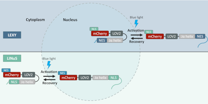
Figure 1: Representation of LEXY and LINuS probes. Both probes consist of a mCherry protein fused to the light-sensitive LOV2 domain. The difference between the two tools resides in the signaling sequence hidden by the Jα-helix: an NES for LEXY and an NLS for LINuS. Both probes also possess a weak signal sequence to control their initial localization: a weak NLS for LEXY and a weak NES for LINuS. The activation of the systems by blue light illumination therefore induces either their export for LEXY or their import for LINuS, allowing users to monitor nuclear export or import. Abbreviations: LEXY = light-inducible nuclear export system; LINuS = light-inducible nuclear localization signal; NLS = nuclear localization signal; NES = nuclear export signal. Please click here to view a larger version of this figure.

The localization of mCherry fluorescence reports the shuttle of LEXY and LINuS probes between nuclei and cytosol, and can therefore be followed in live cell imaging, allowing users to monitor NCT. In addition to being used as simple probes, LEXY and LINuS can also be engineered to control the localization and study proteins of interest, in vitro^5,6,8,9 or in vivo^10,11.

The quantification method proposed in LEXY and LINuS publications shows the relative nuclear intensity of the probes. The suggested analysis is done manually and relies on the measurement of a Region of Interest (ROI) in the nucleus and the cytosol. Although this method gives a good representation of the probe's signal over time, it is very long and tedious, especially when experiments and conditions are repeated. Of importance, this method also lacks accuracy since only a small portion of the designed compartment is represented.

Here we propose a new protocol for LEXY and LINuS fluorescent signal quantification. We implemented automated techniques, which facilitate the analyses and provide greater accuracy. This will ease the process for new users of these tools and help to increase throughput. Our quantification protocol uses only one interface, the open-source TrackMate¹² plugin of FIJI. Notably, to improve the reliability of the quantifications, we used a live-imaging compatible far-red DNA marker to perform whole nucleus segmentation with StarDist¹³, a trained convolutional neural network, combined with tracking and measuring of the probe's fluorescent signal with TrackMate¹².

The data obtained can then easily be exported into the provided and ready-to-use spreadsheet (Supplemental Table S1) to obtain the relative nuclear intensity of each identified nucleus. This protocol also explains how to pool the obtained values in a graph by fitting the time course curve obtained to a monoexponential model, as in Yoo and Mitchison¹⁴ and how to calculate the transport rate for the different conditions tested. With this protocol and the provided spreadsheet for analysis, users will be able to easily quantify live-cell imaging data, even with limited bioinformatics skills.

Protocol

NOTE: The following protocol is described for monitoring nuclear export with LEXY's probe. Details regarding settings to adjust for LINuS are presented in section 5.

1. Cell culture

NOTE: The procedure in this section should be performed in a tissue culture grade hood. The steps described below have been optimized for NIH/3T3 mouse fibroblast¹⁵ cell line, using DMEM (or phenol red-free DMEM when indicated), supplemented with 10% fetal bovine serum and 1% Penicillin-Streptomycin as the medium (see the Table of Materials). However, users can adapt the procedure for other cell types. The protocol is suitable for transfected cells or stable cell lines. However, we recommend creating stable cell lines, as mentioned in the discussion section.

1. Prepare the coating solution with 23 µg/mL collagen and 2 µg/mL fibronectin in sterile 1x PBS. Add 800 µL of the coating solution to each live imaging dish (see Table of Materials) and keep in the incubator for 90 min.
2. Wash the coating mix with sterile 1x PBS and seed 60,000 cells on the live imaging dishes in media, for an acquisition the next day.
3. If needed, transfect the cells with the LEXY plasmid according to the transfection method that best suits the cell type used. To follow this protocol, perform a co-transfection of the probe with an empty vector to increase efficiency, in a ratio of 1:5 for LEXY:empty vector. Protect the cells from light in a dark box or with aluminum foil and let them grow for a day.
4. Before acquisition, stain the cells with a far-red DNA marker compatible with live cell imaging, in a phenol red-free medium, and make sure that they are completely protected from light until the acquisition.
   NOTE: In our case, we use SiR-DNA¹⁶ at 1 µM, incubated for at least 1 h before the acquisitions.
5. To control for export, use the nuclear export inhibitor Leptomycin B¹⁷ at 0.5 nM (mild export inhibition) and 1 nM (strong export inhibition), applied to the cells 1 h before the acquisitions.

2. Imaging

NOTE: Acquisitions can be made with a live imaging compatible confocal microscope, that has the ability to create a pattern of chosen acquisitions and a pulsatile 458 nm laser illumination. Our imaging was performed in the dark in a 37 °C chamber (with 5% CO₂) of a confocal microscope with resonant scanning. The setup is optimized with the 20x objective, therefore allowing simultaneous imaging of multiple cells in the same field of view. The imaging sequence is composed of three phases, as in Figure 2.

1. Stable phase
   1. Perform one acquisition of mCherry (LEXY, 561 nm laser) and far-red (SiR-DNA, 633 nm laser) signals every 15 s, and repeat it 10x, for a total duration of 150 s. Ensure that neither bleaching nor translocation of LEXY to the cytosol are observed at this point.
      CAUTION: An illumination of the system with blue light at this stage would activate LEXY, which would immediately induce its export into the cytosol.
2. Illumination phase
   NOTE: This phase is composed of three steps, repeated 15x.
   1. Carry out pulsatile illumination with blue light (458 nm laser), with 36 ms pulses repeated 150x, for a total duration of ~5 s.
   2. Perform one acquisition of mCherry (LEXY, 561 nm laser) and far-red (SiR-DNA, 633 nm laser) fluorescent signals.
   3. Pause for 15 s.
3. Recovery phase
   1. Perform one acquisition of mCherry (LEXY, 561 nm laser) and far-red (SiR-DNA, 633 nm laser) signals every 15 s, repeat 25x, for a total duration of 375 s.
      NOTE: This step is optional and can be removed if users only want to observe the export of the probe and not the recovery.

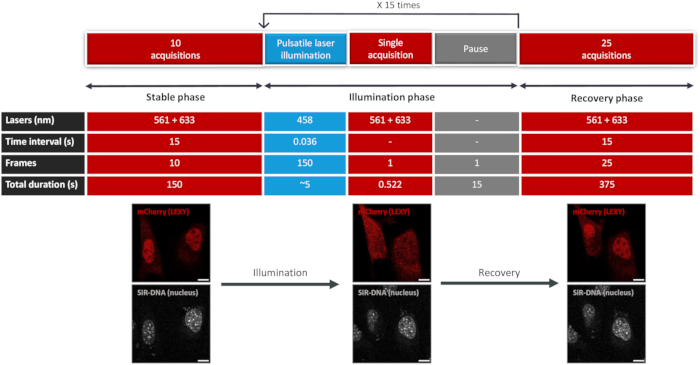
Figure 2: Configuration of the three phases of LEXY. To monitor nuclear export with LEXY, three phases must be set up on the microscope software. The top part indicates the configuration to use for LEXY's live cell imaging acquisitions. This configuration consists of a stable phase, to ensure the signal is stable in the nucleus, an illumination phase, to induce the translocation of LEXY from the nucleus to the cytosol, and a recovery phase, to observe LEXY coming back to the nucleus. The bottom part of the figure indicates the expected results with live cell imaging. In red, the mCherry indicates the localization of LEXY. In grey, the SiR-DNA stains the nucleus of the cells. Scale bars = 10 µm. Please click here to view a larger version of this figure.

3. Analysis for LEXY

NOTE: The whole segmentation and tracking analysis is made using FIJI, with TrackMate¹², an open-source Fiji plugin (version required detailed in the Table of Materials).

1. Install FIJI and then download StarDist¹³ and TrackMate plugins. To install the plugins, go to Help | Update … | Manage Update Sites and tick CSBDeep, StarDist, and Trackmate-StarDist, then click on Apply changes. Restart Fiji.
2. While some microscopes can take each acquisition phase (Stable-Illumination-Recovery) together, others (e.g., the referenced confocal microscope) save them separately. Therefore, an additional step, if using this configuration, is to concatenate the phases together: open the images of the three sequences, run the concatenate function to compile the three time-lapse phases in a single file: click on Image | Stacks | Tools | Concatenate….
3. Select the stable phase as Image1, the illumination phase as Image2, and the recovery phase as Image3. The resulting image is a single image for the time-lapse of the three phases, with the mCherry (channel 1) and SiR-DNA (channel 2) channels merged.
4. Keep the obtained image for the later segmentation step and save it: go to File | Save As | Tiff….
5. Split the mCherry channel alone for the following analyses: go to Image | Color | Split Channels and save it: go to File | Save As | Tiff….
6. To check for eventual bleaching during acquisition, run the Plot Z-axis Profile command on the mCherry channel: go to Image | Stacks | Plot Z-axis Profile. On the generated table, click on Data | Copy 1 ^st Data Set and paste it into the ready-to-use spreadsheet provided with this protocol (Supplemental Table S1), below the Z-axis profile cell.
7. Draw a circular region of interest (ROI) of the average size of a nucleus and save it: go to Analyze | Tools | ROI Manager…. Add the ROI and save it: go to More | Save…
   NOTE: The same ROI should be used to measure the background for all the conditions analyzed.
8. Place the saved ROI in a region without cells during the whole time-lapse and measure the average intensity within this ROI with the ROI interface function. First, make sure that the mean grey value is ticked by clicking on Analyze | Set Measurements. Then, click on More | Multi Measure. Tick Measure all 50 slices and one raw per slice, and click on ok.
9. Copy-paste all the values displayed in the provided spreadsheet (Supplemental Table S1), below the "ROI Background" cell.
10. In Fiji, close the image with only the mCherry channel and select the previously saved image with the merged mCherry and SiR-DNA channels.
11. Open the TrackMate plugin: go to Plugins | Tracking | TrackMate.
12. Check that the number of time points is correct (0 to 49 if the proposed phases were followed) and click on Next.
13. Select the StarDist detector and click on Next.
14. Select channel 2 (SiR-DNA) to segment the nuclei and click on Next. Wait a few seconds for the segmentation process to finish. Visually inspect that the obtained segmentation corresponds to the border of the nuclei and click on Next (Figure 3). In case of inaccurate segmentation, take note of the corresponding nucleus identifier (SpotID) to exclude it from further analysis in step 3.26.
15. Leave the default parameters and click on Next on the initial thresholding setting window. This window gives the number of segmented spots (nuclei) among the 50 time points.
16. Set filters on spots: create and set filters:
    1. Create two filters with Mean intensity ch1 as a parameter to remove nuclei with too intense or too weak signal, which could skew the analyses: one filter to select values above the defined threshold and the other to select the values below the threshold. Define the value to only remove the very low or saturated signal.
       NOTE: These filters might not be needed if stable cell lines are used. Note these values as they need to be reapplied for all the conditions.
    2. Create two filters Area to remove undesired objects (debris, dying or dividing cells) from analyses: one filter to select values above the defined threshold and the other to select the values below the threshold. Click on Next.
       NOTE: Reapply these values for all the conditions.
17. Select a tracker: choose Simple LAP tracker and click on Next.
18. Select the parameters for the tracking. Adjust the Linking max distance (here, 30 µm)-the maximum distance that will be allowed to link to objects between frames. Use the Gap-closing max distance (here, 15 µm) and Gap closing max frame gap (here, 3) to define how many spots of a single track can be omitted without excluding this same track. Click on Next (Figure 3).
    NOTE: These proposed parameters were optimized for our setup and cellular model using a trial-and-error approach and might need to be adjusted experimentally.
    Linking max distance needs to be adjusted to prevent mistracking from one nucleus to another, especially if the cells move a lot.
19. After calculations, click on Next and set filters on tracks. To only select nuclei that have been tracked during the entire time course (50 time points with the proposed sequence), select the highest number of spots in the track (place the cursor on over 49 for the proposed sequence). Click on Next.
    NOTE: This will facilitate the analysis but is only possible if enough nuclei have been tracked for the entire time course, if not: see discussion.
20. Display options: tick Display spot names to be able to retrace each nucleus in further analyses. Customize the displayed features according to the user's preferences.
21. On the bottom of the page, click on Tracks | Export to CSV to save the table with all the measurements. Close the table and click on Next.
22. Optionally, plot the track features with T (time) as the X axis and the Mean intensity of the ch1 for the Y axis. Click on Plot features. Close the graph and click on Next.
    NOTE: This will give the users an idea of the general tendency of the export. At this point, it is not normalized to the background and initial intensity.
23. Click on Capture overlay as action and Execute | OK. The image generated will be used to identify the quantified nuclei. Save: go to File | Save As | Tiff….
24. In a spreadsheet file, import the CSV file obtained with TrackMate: On the Data tab, in the Get & Transform Data group, click From Text/CSV and Import.
25. Select the whole four following columns by clicking on their corresponding letter and copy and paste them at the top of the provided spreadsheet (Supplemental Table S1), columns A to D, with the background: Spot ID (B), Track ID (C), Frame (I), Mean intensity ch1 (M).
    NOTE: Ensure that the beginning of the measures pasted starts at row 6 of Supplemental Table S1. If this is not the case, the measurements could be shifted from one or more cells and therefore be incorrect. Refer to the spreadsheet of Supplemental Table S2 to have an example of the expected disposition.
26. Sort the results alphabetically first by TrackID (individual nucleus) by clicking on the arrow in cell B5 and Frame (time point) by clicking on the arrow in cell C5.
27. To remove background noise, subtract the values obtained in step 3.8 from each value obtained in Mean intensity ch1 (precalculated in the provided spreadsheet, see Supplemental Table S1).
28. To normalize LEXY's signal, calculate the mean intensity of the mCherry fluorescent signal in the stable phase (frames 0 to 9). Then, divide all the results obtained in Mean intensity ch1 by the mean intensity of the stable phase (precalculated in the provided spreadsheet, see Supplemental Table S1).
    ​NOTE: The number obtained is the mean nuclear fluorescent intensity of LEXY. All measures are already displayed by nuclei from column L and can be plotted in a graph.

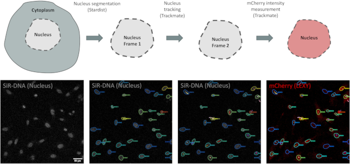
Figure 3: TrackMate analysis using FIJI. On top, schematic representation of the TrackMate analyses, on the bottom, images obtained from the FIJI analyses. The first representation on the left shows the unsegmented SiR-DNA staining, a marker of the nucleus, in grey. The second panel represents the automatic segmentation performed with the SiR-DNA channel by Stardist. The nuclei are colored according to the intensity of the mCherry channel, to facilitate the visualization and the final step. The third panel shows the tracks obtained by tracking SiR-DNA staining in the timepoints of the whole live cell imaging sequence. The last panel on the right shows LEXY's fluorescent signal, in red, in the area defined by the segmentation, which will be measured for each time point. Scale bar = 50 µm Please click here to view a larger version of this figure.

4. Transport rate, statistics, and figures

1. Plot the relative nuclear intensity graph.
   1. Open GraphPadPrism and create a sheet: click on Enter or import data into a new table, and in the options, select elapsed times for X and the maximum number of segmented nuclei for the replicate values in side-by-side subcolumns for Y. Click on Create and paste the obtained data in the table.
   2. For the X values (time), if the parameters of acquisitions were kept as suggested, copy and paste the column under 'time' in the provided spreadsheet. Otherwise, adjust the values according to the parameters used.
   3. To create the graph of the relative nuclear intensity, go to the Graphs section. Select XY as the graph family, and Points & connecting line with error bars as the graph type.
   4. In the Plot section, select Mean, Error, and SEM and click on OK to see the graphs. Change the scales and visuals according to the chosen parameters.
2. Fit the relative nuclear intensity to a monoexponential model.
   1. In the Data Table section, click on New Data Table.
      1. Select Enter X values as X and Enter and plot a single Y value for each point as Y, and click on Create.
      2. In the X column, report the times in decimals only for the stable and illumination phases; if the suggested parameters of acquisitions were kept, copy and paste the column under 'decimal time' in the provided spreadsheet, Supplemental Table S1.
      3. Paste the values obtained as relative nuclear intensity in the table, only for the stable and illumination phases.
      4. In the Results section, select the following analysis: XY analyses | Exponential | Nonlinear Regression (Curve Fit) and click on OK.
      5. In the parameters, select Plateau followed by one phase decay as Model, and in the constrain parameters, select a constant equal to 2.25 as X0 (the starting time of illumination), a constant equal to 1 as Y0 (relative nuclear intensity at the beginning of illumination), a constant equal to 0 for the plateau (the values towards which the relative nuclear intensity should lean on), and indicate that K (the export rate), should be greater than 0. Leave the other parameters on default. Click on OK.
      6. In the Results section, the K row indicates all the export rates for the nuclei of the tested condition.
      7. Repeat steps 4.2.1 to 4.2.1.5 for the other conditions if needed.
3. Create the export rate graph.
   1. Create a new table: select Enter X values as X and Enter and plot a single Y value for each point as Y, and click on create.
   2. For each condition (in columns), paste and transpose the K values obtained in the previous step.
   3. To create the graph of the export rate, go to the Graphs section, select column as graph family, and in the Box and violin section, select Violin plot as graph type, with Violin plot. Show all points as plot. Click on OK to see the graph. Customize the way of representing the data if needed.
   4. To run a statistical test for the export rate, perform a two-sided Welch's t test,as described in Yoo and Mitchison¹⁴, by following the next steps:
      1. In the table containing the export rates of all the conditions, click on Analyze | Group Comparison | T-Test (and nonparametric tests), select the conditions to be tested, and click on OK. Tick Unpaired, Yes use parametric test, and Unpaired t test with Welch's correction. Do not assume equal SDs, and click on OK.
   5. Observe the results of the analysis in the table of the Results section and report on the export rate graph if required.

5. Adaptations for LINuS

NOTE: The protocol described above can easily be adapted to monitor nuclear import with LINuS by applying the following changes.

1. Cell culture
   1. Instead of Leptomycin B in step 1.5, use importazole¹⁸ as the nuclear inhibitor, at a concentration of 10 µM for 1 h before the acquisition.
2. Imaging
   1. To have an optimal import of the system, replace the 150 repetitions of 36 ms pulses of illumination by the 458 nm laser in step 2.2.1 by 250 repetitions for a total duration of ~9 s.
      NOTE: the sequence timing can be cell type-dependent, and the parameters for both probes might need adjustment to be optimal, since the systems depend on the recognition of NLS and NES, which are cell type-specific^19,20.
3. Transport rate, statistics, and figures
   1. Instead of fitting a curve to a Plateau followed by one phase decay in step 4.2.1.5, select the Plateau followed by one phase association analysis.
   2. Constrain X0 to 2.25, Y0 as 1, and K (the import rate in case of LINuS) greater than 0.
      NOTE: LINuS's analyses with TrackMate are identical to LEXY's. The relative nuclear intensity is still the value measured and analyzed, but instead of observing a decrease due to the probe's export, an enrichment of the fluorescent signal in the nucleus after blue light illumination should be observed.

Results

The above-mentioned protocol should allow the users to visualize the probe's localization and translocation during the acquisition in live cell imaging. An example of the expected images acquired to visualize nuclear export with LEXY is shown in Figure 4. A rapid decrease of the signal from the nucleus and an enrichment in the cytosol should be observed after a couple of rounds of blue light illumination. A progressive recovery of the probe's signal can be visible after stopping the illumination cycles. To control the system, Leptomycin B, an export inhibitor, attests that a change in export can be visualized with the analyses, since it prevents LEXY from being exported upon blue light illumination (Figure 4).

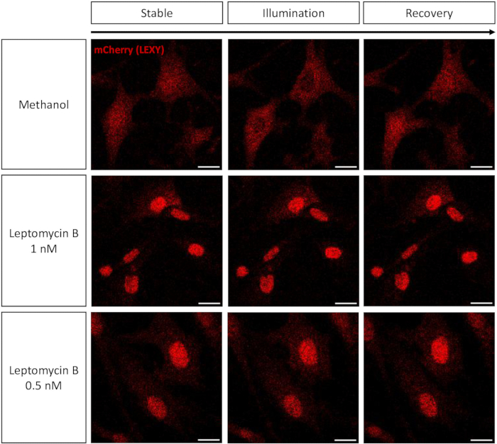
Figure 4: Visualization of LEXY's signal over time. Capture of representative time points of the stable, illumination, and recovery phases, acquired with live cell imaging. The methanol condition represents the control condition. Upon pulsatile blue light illumination, in red, the mCherry fluorescent signal, reporter of LEXY's location, is translocated from the nucleus to the cytosol. After stopping the illumination, the signal is recovered in the nucleus. Treatment with the export inhibitor Leptomycin B at 1 nM or 0.5 nM shows the absence or decrease of LEXY's export when the export is blocked. Scale bar = 30 µm. Please click here to view a larger version of this figure.

Regarding the analyses, while values of the relative nuclear intensity curve during the stable phase should be around 1, after blue light activation, they should display a slow decrease until reaching a plateau at the end of the illumination phase (Figure 5A). If the decrease is too fast or too slow, acquisition parameters can be optimized (see discussion). Leptomycin B treatment at sufficient concentrations can also confirm that the analyses and technique are sensitive enough to show that nuclear export is completely blocked, with relative nuclear intensity values stable at around 1 for the whole experiment. Intermediate Leptomycin B concentrations, however, should display a mild nuclear export (Figure 5A). These visual observations should be confirmed quantitatively with the obtention of the export rate (Figure 5B).

Figure 5: Expected relative nuclear intensity of LEXY and transport rate. (A) The graph represents the relative nuclear intensity of LEXY's fluorescent signal over time, normalized to the mCherry mean intensity of the stable phase. The relative nuclear intensity of the methanol (control, red) condition decreases by half after illumination, in contrast to the cells treated with the export inhibitor Leptomycin B, at a concentration of 0.5 nM (light blue) or 1 nM (dark blue). Error bars: SEM. (B) Export rate of the control and Leptomycin B conditions, obtained by fitting the curve to a monoexponential model. The values obtained when the export is blocked by Leptomycin B are significantly lower than the control condition. N = 18 cells for Methanol (red), 19 cells for Leptomycin B 0.5 nM (light blue), and 15 cells for Leptomycin B 1 nM (dark blue). P values were calculated by a two-sided Welch's t test. ***: P < 1×10⁻⁴, ****: P < 1×10⁻⁵. Please click here to view a larger version of this figure.

Supplemental Table S1: Spreadsheet with predefined calculations. This spreadsheet is provided to facilitate the analysis. The intensity values obtained with TrackMate can be directly copied and pasted into the spreadsheet to obtain the normalized relative nuclear intensity values. Please click here to download this File.

Supplemental Table S2: Example of the expected results for a control condition of LEXY's analysis. The spreadsheet represents an example of the obtained values for a control condition of LEXY's stable cell line. Please click here to download this File.

Discussion

As mentioned in the protocol, the creation of stable cell lines greatly improves the quality of the analyses. First, having 100% of the cells expressing the probes increases the number of nuclei tracked and analyzed, which strengthens the robustness of the analyses. Second, it reduces cell death induced by the overexpression of the probes and the toxicity of the transfection reagents used. And finally, it reduces the strong heterogeneity of fluorescent signals amongst the cells. This parameter is of importance since a saturated signal will not allow proper detection of the change of intensity after illumination. The same conclusion is true for weak signals, which may bleach or not allow for the quantification of differences. Therefore, we recommend first testing the probes by transfection to ensure that they work properly, setting up the acquisition parameters, and then rapidly creating stable cell lines. We created lentivirus vectors for both LEXY and LINuS probes, which are available to share upon request, as well as the NIH/3T3 LEXY or LINuS stable lines created with these lentiviruses.

If the probes are transfected or if cells are sparse, the parameters suggested will likely decrease the number of tracks detected, and the analyses will be less robust. If this is the case, the users can be more permissive with the spots omitted in the tracking by decreasing the filter Number of spots in tracks (we suggest keeping at least 45 out of 50 spots). Caution: if this filter is decreased, the Excel file provided (Supplemental Table S1) should be manually adjusted: indeed, the values pasted from the CSV imported will not take into account the gaps. The user needs to find where the missing spots are with the TrackID number and correlate them with the nucleus number, which usually takes a few copy-paste rounds.

A critical parameter to guarantee the success of the experiment is to keep the cells in the dark. As the probes react to blue light, users must ensure the transport of the cells in the dark for at least 30 min before acquisition. A small closed box or using aluminum to cover the dish is sufficient. Similarly, it is necessary to be very careful to only use the mCherry light to search for the cells at the microscope, since illumination with blue light activates the cells. If an eventual illumination happens under the microscope, search for another distant field for the acquisition. Plotting the Z-axis Profile in step 3.6 will help to know if the cells were impacted by an illumination, if the curve is decreasing instead of being a plateau.

The imaging sequence is set up to consist of three phases. First, the stable phase, to assess for potential bleaching but also to ensure that LEXY's localization is steady without activation (1). Second, the activation phase, consisting of rounds of pulsatile blue light illumination, to induce the translocation of LEXY from the nucleus to the cytosol (2). Finally, the optional recovery phase, where the signal progressively goes back to its initial location in the nucleus (3).

The sequence described for acquisitions can be cell-type-specific^19,20. For the first experiment, the user should test and modify the laser power and timings to see the system progressively translocate between the nucleus and cytosol. Of importance, a laser power too strong, as a pause too short, might prevent seeing a progressive translocation, but instead a brutal drop/enrichment (depending on the probe used) of the mCherry intensity after illumination.

If the sequence's optimization does not solve the problem, it is likely that the NES and/or NLS are not suited for the cell type used. Users can refer to the LINuS method article⁸ to engineer and modify the probes. Users can also consult this article for imaging LINuS with an epifluorescence microscope.

The nuclei segmentation is a critical step of the analysis. A robust and reliable nuclear marker should be used for live cell imaging of the probes. Since illumination with blue light activates the probe's translocation, and because the probes are monitored with mCherry fluorescent protein, this marker must be visible in the far-red spectrum or close. In our case, we use SiR-DNA that stains the cells during 1 to ~24 h of incubation, but using SPY-DNA 650 is also an option (see Table of Materials for references).

Finally, if the segmentation with StarDist combined with the filtered tracking of TrackMate proves its efficiency, it is important to note that the user should always visually check the results of the segmentation and the quantification. A dividing or dying cell might be included in the quantification, whereas it should not. To reduce the risks of analysis of such events, the provided Excel sheet attributes a color code to the relative nuclear intensity (blue = low values, red = high values). By inspecting the colors before plotting the values in GraphPad Prism, the user should be able to notice any unusual values. For example, LEXY's relative nuclear intensities should vary from high (red, strong amounts of the probe in the nuclei) during the stable phase to low (blue, reduced amounts of the probe in the nuclei) at the end of the illumination phase, before coming back to high values (red), at the recovery phase (as displayed in the Supplemental Table S2).

This protocol presents various advantages over previously proposed methods^5,6. The semi-automatic pipeline facilitates the analysis of LEXY and LINuS nucleocytoplasmic transport, and provides more accuracy than previously proposed manual quantification^5,6. Using our protocol will enable beginners in the field to perform efficient analyses, but also provide a new tool for experienced users, who will need only one open-access interface to perform semi-automated analyses of the nucleocytoplasmic transport.

This method can be used for further applications than the study of global nucleocytoplasmic transport rate in NIH3T3 cell lines. Indeed, with a few optimization steps, it can be adapted to study the probe's transport rate in various cell types or living animals⁸. Furthermore, by fusing a protein of interest to either LEXY or LINuS, it is also possible to study its transport rate or the downstream effects of its light-induced translocation in or out of the nucleus. For example, it is possible to sequester a protein in the cytoplasm with LEXY, or to force its localization into the nucleus with LINuS^5,6,21,22,23. Finally, the analyses described can also be extended to more applications than LEXY and LINuS, to track any signal that translocates between subcellular compartments that can be segmented.

Materials

List of materials used in this article

Name	Company	Catalog Number	Comments
Collagen	Sigma-Aldrich	08-115
Confocal microscope	LEICA	SP8
DMEM	Gibco	31966021
Excel	Microsoft
FBS	Sigma-Aldrich	F7524
Fibronectin	Sigma-Aldrich	F1141
FIJI software	FIJI		ImageJ 2.16.0/1,54p; Java1.8.0_322
Fluorodishes	Dutscher	FD3510-100	Alternative: Attofluor chamber (Invitrogen #A7816)
GraphPad Prism 10.4.1	GraphPad Software, Inc.
Importazole	Sigma-Aldrich	SML0341
Leptomycin B	Sigma-Aldrich	L2913
LEXY plasmid	Addgene	72655	pDN122
LINuS Plasmid	Addgene	61347	pDN77
Pencillin-Streptomycin	Gibco	15140-122
Phenol-red free DMEM	Gibco	21063-029
SiR-DNA	Spirochrome	SC007	Alternative: SPY-DNA650 (Spirochrome #SC501)
Stardist 2D plugin	StarDist		StarDist_0.3.0
TrackMate plugin	TrackMate		TrackMate-7.14.0

References

- Wing, C. E., Fung, H. Y. J., Chook, Y. M. Karyopherin-mediated nucleocytoplasmic transport. Nat Rev Mol Cell Biol. 23, 307-328 (2022).
- Kelley, J. B., Paschal, B. M. Fluorescence-based quantification of nucleocytoplasmic transport. Methods. 157, 106-114 (2019).
- Crefcoeur, R. P., Yin, R., Ulm, R., Halazonetis, T. D. Ultraviolet-B-mediated induction of protein-protein interactions in mammalian cells. Nat Commun. 4 (2), 1779(2013).
- Beyer, H. M., et al. Red light-regulated reversible nuclear localization of proteins in mammalian cells and zebrafish. ACS Synth Biol. 4 (9), 951-958 (2015).
- Niopek, D., et al. Engineering light-inducible nuclear localization signals for precise spatiotemporal control of protein dynamics in living cells. Nat Commun. 5, 4404(2014).
- Niopek, D., Wehler, P., Roensch, J., Eils, R., Di Ventura, B. Optogenetic control of nuclear protein export. Nat Commun. 7, 10624(2016).
- Zayner, J. P., Antoniou, C., Sosnick, T. R. The amino terminal helix modulates light activated conformational changes in AsLOV2. J Mol Biol. 419 (1-2), 61-74 (2012).
- Wehler, P., Niopek, D., Eils, R., Di Ventura, B. Optogenetic control of nuclear protein import in living cells using light-inducible nuclear localization signals (LINuS). Curr Protoc Chem Biol. 8 (2), 131-145 (2016).
- Lataster, L., et al. Cell cycle control by optogenetically regulated cell cycle inhibitor protein p21. Biology. 12 (9), 1194(2023).
- Forlani, G., et al. Analysis of slow-cycling variants of the light-inducible nuclear protein export system LEXY in mammalian cells. ACS Synth Biol. 11 (10), 3529-3533 (2022).
- Inutsuka, A., Kimizuka, N., Takanohashi, N., Yakabu, H., Onaka, T. Visualization of a blue light transmission area in living animals using light-induced nuclear translocation of fluorescent proteins. Biochem Biophys Res Commun. 522 (1), 138-143 (2020).
- Tinevez, J. -Y., et al. TrackMate: An open and extensible platform for single-particle tracking. Methods. 115, 80-90 (2017).
- Schmidt, U., Weigert, M., Broaddus, C., Myers, G. Cell detection with star-convex polygons. Medical Image Computing and Computer Assisted Intervention - MICCAI 2018. Frangi, A. F., Schnabel, J. A., Davatzikos, A. F., Alberola-López, C., Fichtinger, G. , Springer International Publishing. Cham. 265-273 (2018).
- Yoo, T. Y., Mitchison, T. J. O-GlcNAc modification of nuclear pore complexes accelerates bidirectional transport. J Cell Biol. 220 (7), e202010141(2021).
- Jainchill, J. L., Aaronson, S. A., Todaro, G. J. Murine sarcoma and leukemia viruses: assay using clonal lines of contact-inhibited mouse cells. J Virol. 4 (5), 549-553 (1969).
- Lukinavičius, G., et al. SiR-Hoechst is a far-red DNA stain for live-cell nanoscopy. Nat Commun. 6, 8497(2015).
- Kudo, N., et al. Leptomycin B inactivates CRM1/exportin 1 by covalent modification at a cysteine residue in the central conserved region. Proc Natl Acad Sci U S A. 96 (16), 9112-9117 (1999).
- Soderholm, J. F., et al. Importazole, a small molecule inhibitor of the transport receptor importin-β. ACS Chem Biol. 6 (7), 700-708 (2011).
- Henderson, B. R., Eleftheriou, A. A comparison of the activity, sequence specificity, and CRM1-dependence of different nuclear export signals. Exp Cell Res. 256 (1), 213-224 (2000).
- Lu, J., et al. Types of nuclear localization signals and mechanisms of protein import into the nucleus. Cell Commun Signaling. 19 (1), 60(2021).
- Krueger, D., et al. Principles and applications of optogenetics in developmental biology. Development. 146 (20), dev175067(2019).
- Kögler, A. C., et al. Extremely rapid and reversible optogenetic perturbation of nuclear proteins in living embryos. Dev Cell. 56 (16), 2348-2363 (2021).
- Zhang, W., et al. Hitchhiking of Cas9 with nucleus-localized proteins impairs its controllability and leads to efficient genome editing of NLS-free Cas9. Mol Ther. 32 (4), 920-934 (2024).
Reprints and Permissions