Optically Trapping Large Metallic Particles in Air Using a 'Boat' Trap with Direct-Drawn Sidewalls

Summary

This paper describes the experimental method for achieving long-duration, stable trapping and precise positioning of large metallic particles in air using a dynamic, boat-shaped photophoretic trap. This system enables controlled manipulation that is suitable for plasmonic interaction studies.

Abstract

We present a method for achieving stable optical trapping of large metallic particles (>1.16 µm mean diameter solid gold particles, and >100 μm conductor-coated microspheres) using a focused beam, scanned by acousto-optic modulators to directly draw a parabolic trap cross-section in the air.  The result of this drawing action is the formation of a 'boat' trap, open on top, capable of catching, loading, and stably holding large metallic particles without hopping.  A high-power continuous-wave 532 nm laser is scanned in both the x- and y-directions, forming a boat-shaped intensity distribution optimized for trapping microspheres. The trapping duration is maximized by careful selection of drawing frequency to be fast enough to appear continuous relative to particle dynamics, but slow enough to avoid trap distortion. This protocol describes the experimental setup, including laser modulation, particle introduction techniques, and validation. Carbon-coated microspheres are used primarily to visualize and validate trap formation and stability, while solid gold nanoparticles serve as the target for plasmonic interaction studies. This method allows for any one of a number of cross-sections to be drawn on command, in real-time, to provide a robust, flexible approach for capturing, loading, and translating airborne particles over long timescales, with potential applications in plasmonic enhancement of levitated optical systems. 

Introduction

This work presents a method for the precise capture, placement, and manipulation of large metallic particles in air using a dynamically generated boat trap. Prior approaches—such as those employing loosely focused Gaussian beams¹, aberration traps², speckle fields^3,4,5, or vortex beams^6,7—suffer from key limitations, including rotational motion¹, multiple stable trapping loci^2,3,4,5, or a lack of a single, well-defined trapping site^6,7, which, in some geometries, may lead to hopping between multiple stable trapping loci^3,7 (see Figure 1A).  One noteworthy exception is the upward-directed axicon trap, which provides a single trapping locus, supports top-loading, and—at least theoretically—permits lateral translation⁸. The method described here retains those advantages while introducing three critical improvements: (1) robust trapping of metallic particles, (2) a horizontal beam geometry, and (3) real-time reconfigurability of the trapping potential via direct-drawn optical walls. 

Approaches for trapping gold particles to date have typically been performed in water^9,10,11, may have trap characteristics that impart rotational motion¹², or employ counter-propagating beams that inhibit the flexible translation of a trapped particle¹³. To overcome these challenges for solid gold particles with diameters greater than 1 μm, a dynamically modulated photophoretic 'boat' trap is employed.  

This method is applicable to a wide range of particle sizes and types, from 20 nm carbon nanosphere clusters to 100 µm coated glass microspheres. It is effective in both open ambient and closed partial-pressure environments. The technique can operate at powers up to several tens of Watts.  Because the traps are distributed as lines rather than points, with optical power spread over large areas, practical implementation is most effective at powers above 1 W.

The trapping mechanism relies on positive photophoresis, which arises from asymmetric heating of the particle by the laser beam. When an absorbing metallic particle is illuminated, the hotter side emits gas molecules with greater momentum than the cooler side, resulting in a net force that pushes the particle away from the light. This photophoretic force can be expressed as:

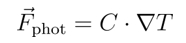
where C  is a coefficient that depends on the particle geometry, gas properties, and thermal accommodation coefficient, and ∇T is the temperature gradient along the particle surface. In this system, this force is directed upward in the trap and counteracts gravity, allowing stable levitation. A more detailed derivation of the photophoretic force—including both radiometric pressure and thermal creep effects—is provided in Mirzaei-Ghormish et al.¹⁴.

The boat trap uses an arbitrary waveform generator (AWG) to control acousto-optic modulators (AOMs) to form a high-intensity optical wall created by scanning a focused continuous wave (CW) laser beam to generate a stable parabolic trapping potential¹⁴ (see Figure 1B).  This approach enables precise control of the trap shape, allowing particles to be trapped, held still, and exposed on one surface—key requirements for applications such as bringing nanodiamonds close to gold plasmonic particles of dimension greater than 1 μm for Purcell enhancement of nanodiamond fluorescence¹¹

Protocol

This section describes the preparation of particles and the construction of the optical setup. Note that this setup differs from vortex, diffracting, and other wavefront shaping approaches, which result in a single trap morphology (see Gong et al. for a review of wavefront shaping traps⁸). In this setup, by scanning a focused point primitive, one can create many trap cross-sections. Therefore, while this work emphasizes the boat trap morphology, be aware that the setup described is flexible enough to create many other trap geometries to be treated in future work.

1. Preparation of particles

1. Carbon-coated glass microspheres (used for visualization, Figure 2)
   1. Transfer 3 mL of microspheres into a small, clean crystallization dish (Figure 2A, left) using a clean spatula. Perform this step in a fume hood to prevent bulk dispersal of fine glass particles.
      NOTE: The fume hood maintained negative pressure, drawing air inward with an average face velocity of 101 ft·min^-1.
   2. Cover the dish with a lid or watch glass and transfer to a carbon rod evaporation system (Figure 2B).
   3. Set the evaporation routine to 3 pulses at 73 A pulse current, 3 s pulse length, and 10 s pulse interval (See Table 1).
   4. Remove the lid. Insert particle dish. Run the coating program. Replace the lid. Remove the dish.
   5. Agitate the dish by shaking the particles with sufficient force to randomize the particle positions (Figure 2C). Remove the lid and place the dish back in the coater for coating. Repeat 10 times.
      NOTE: After coating, the particles will look like those in Figure 2A, on the right-hand side. Note also that the resultant size of the carbon-coated microsphere is practically unchanged, as the 20 nm coating is small compared to the average diameter of a carbon-coated microsphere, which can exceed 60 µm.
   6. Cover the resulting particles with a watch glass or film and keep them in a humidity-controlled environment.
      NOTE: All coating and experimental work was performed in an environment maintained at indoor lab conditions with a temperature of 21-25 °C (70-75 °F) and 20-45% relative humidity.
2. Solid gold particles (used for plasmonic experiments)
   1. Solid gold particles are sold dry with average diameters of 1 µm (see Figure 2D and Table of Materials). When ready to use, transfer the dried particles into the rotating glass particle chamber (Figure 2E).

2. Setup of optical system

NOTE: The optical setup is shown in Figure 3. The complete list of required optical and electrical components to complete the setup is provided in Table of Materials. In this setup, four identical lenses create two cascaded 4F relays that image AOM₁ onto AOM₂. AOM₁ deflects the beam vertically, AOM₂ deflects it horizontally, and because the focal lengths are equal, the conjugate plane of AOM₁ coincides with AOM₂.

1. Laser source and initial beam alignment
   1. On an optical table, place a laser source capable of powers from <5 mW to >5 W of 532 nm light output.
      NOTE: The source laser used in these experiments was capable of trap powers in excess of 10 W. At the output of the laser and prior to entering AOM¹, the beam is collimated with a diameter of approximately 1.3 mm (1/e² intensity width), measured using a beam profiler. A 532 nm source was selected because it is available in high powers with good beam quality and has good plasmonic absorption for the target particles.
   2. Reduce laser power to <5 mW. Use a polarizer to determine if the polarization is vertically oriented. If it is not, rotate the laser or insert and rotate a high-power half-wave plate to ensure vertical polarization orientation. Use a kinematic beam elevator (Figure 4A, right side) and a ruler to set the beam height to 23 ± 0.5 cm (this height is arbitrary but has proven to be convenient). Measure the beam height at 10 cm from the elevator and at 40 cm. Ensure that both of these measurements give a height of 23 cm.
      NOTE: The AOM operates using a slow shear mode birefringent acousto-optic interaction in tellurium dioxide (TeO₂), which requires the input beam to be horizontally polarized. The diffracted beam emerges with vertical polarization due to the birefringent nature of the interaction. Since the first AOM is physically rotated by 90° relative to the global coordinate system, the input beam must be vertically polarized in global coordinates to align with the AOM's internal horizontal polarization axis.
2. Objective and relay lens placement
   1. Adjust the microscope to beam height, facing in the -z direction, at a distance greater than 100 cm from the output of the beam elevator (Figure 4A,B).
   2. Place a Fourier transform lens 10 cm in the -z direction with a convex surface facing in the +z direction (Figure 4C,D).
   3. Place the remaining three Fourier transform lenses 20 cm apart with convexities alternating as shown in Figure 4E.
3. AOM configuration
   1. Position AOMs 10 cm in the -z direction from the lenses closest and furthest from the laser, as shown in Figure 5,B.
   2. Ensure that AOM₁ (the AOM closest to the laser) is vertically oriented.
      NOTE: In this instantiation, a custom 3D printed holder was created for this purpose. Rotate AOM₁ approximately 2° toward the optical axis as shown (Figure 5A).
   3. Place AOM₂ 10 cm from the lens furthest from the laser. This AOM will be oriented horizontally (Figure 5B). Rotate AOM₂ approximately 2° away from the optical axis as shown (Figure 5B).
   4. Turn the laser on to a low power (e.g., <5 mW).
   5. For each channel of the AWG, connect a voltage-controlled oscillator (VCO), an amplifier, and one AOM (Figure 5C). First, connect the amplifiers to the AOMs as shown in Figure 5D, E.
      NOTE: It is important to make sure the amplifiers are connected to a load before they are powered on. Amplifiers and VCO's both take 12 V DC power and can be connected to a common 12 V source with banana clips as shown in Figure 5F.
4. AOM optimization
   1. Place an aperture in the system as shown in Figure 6A.
   2. Using the AWG, turn the radio frequency signal to both AOMs to a value of 175 MHz (~5 V on the VCO).
      NOTE: There will now be two beams after AOM¹ and four beams after AOM² (see Figure 6B).
   3. Decrease the tilt angle of AOM₁ to zero. Gradually increase the angle until the first-order beam (the top right' pass beam' which appears when looking in the -z direction as shown in Figure 6C) is at its brightest. The AOM will have returned to approximately the original tilt angle of 2°.
   4. Decrease the tilt of AOM₂ to zero. Gradually increase the angle until the first-order beam is at its brightest. The AOM will have returned to approximately the original tilt angle of 2°.
      NOTE: The average diffraction efficiency (when driven at 1 W electrical power) was approximately 70% for each AOM. Total system optical efficiency was approximately 30%.
   5. Ensure that both beams exiting the first AOM enter the second. Ensure that of the four beams entering the second AOM, the top right beam is chosen to pass through an aperture.
      NOTE: The aperture must be small enough to obstruct the 'block beams' and allow the 'pass beam' to proceed even when deflected by the AOM (Figure 6C,D).
   6. Place a beamsplitter as shown in Figure 6E to direct a portion of the beam to an observation surface (Figure 6E,F).
5. AWG control
   1. With AWG amplitudes set to zero (or AWG outputs set to 'off'), the resulting beam at the observation surface will look like a dot (Figure 7A,B).
   2. Set the vertical channel offset to 3 V, amplitude to 5 V, and frequency to 4 kHz to see a vertical line (Figure 7C,D).
   3. Set the horizontal channel offset to 3 V, amplitude to 5 V, and frequency to 4 kHz to see a diagonal line (Figure 7E,F).
   4. Set the vertical channel frequency to 8 kHz and phase offset to 90° to see a Lissajous pattern (Figure 7G,H).
   5. Press the align phase button to convert the Lissajous pattern to a parabolic shape (Figure 7I,J).
   6. Adjust the vertical channel phase offset to refine the parabolic shape (Figure 7K,L).

3. Imaging system setup

NOTE: The imaging system allows for axial (i.e., ' head-on'), rear-illuminated viewing of particles and the trap profile.

1. Camera, filter, and interface
   NOTE: The camera has a nominal maximum speed of 751 fps; however, the actual rate will vary dramatically with chosen resolution and system latency. In these experiments, the actual rate was approximately 500 fps. Playback was most useful at 1/100th speed or 5 fps (assuming no frames were dropped at capture).
   1. Place a telecentric lens on a linear stage (movable along the z-axis) with a 45 mm focal length, 55 mm in front of the objective (+z direction, Figure 8A). Place a dichroic filter designed to reflect 532 nm light (see Table of Materials) in front of the lens as shown in Figure 8A,B.
   2. Connect the camera by USB to a PC with associated imaging software (see Table of Materials for type and brand. See Table 2 for initial camera settings).
   3. Tilt the dichroic filter slightly (5-10 °) until the parabolic trap shape appears  (Figure 8C,D).
   4. Place the camera on a linear stage (Figure 8E) and move the lens back to refine the image focus (Figure 8F).
   5. Illuminate the beamsplitter with a fiber light source (Figure 8G).
   6. Adjust the fiber light to center its illumination around the parabolic trap (an example of off-centered illumination in Figure 8H, and on-center in Figure 8I).

4. Particle loading and trapping

1. Using a laboratory spatula, place a small quantity (~1 g) of particles inside a 25 mm long, 12 mm diameter glass cylinder mounted to allow rotation along the cylinder axis (Figure 9A).
2. Place the loaded glass cylinder centered at 15 mm (i.e., objective working distance) away from the objective (Figure 9B).
3. Rotate the cylinder  (Figure 9C), tap the cylinder, and observe the camera display. As the user taps, they may observe the following states: default/no trapped particles (Figure 9D), particles falling (Figure 9E), and particle(s) trapped (Figure 9F).

5. Computational tracking with OpenCV

NOTE: Particle tracking and retention time quantification were performed using a custom OpenCV-based program (OpenCV version 4.6.0) developed in C++ and executed in Microsoft Visual Studio 2022.

1. Install software
   1. Install Visual Studio 2022 Community Edition (if the user's use case allows it) at https://visualstudio.microsoft.com/downloads/. Install the Desktop development with C++ workload.
   2. Download and install OpenCV. https://github.com/opencv/opencv/releases. While installing, take note of the installation directory.
   3. Download and install NI VISA. https://www.ni.com/en/support/downloads/drivers/download.ni-visa.html One has to make an account to install it. While installing, take note of the installation directory.
   4. Download and install Pylon version 7.5.0.15658. https://www.baslerweb.com/en-us/downloads/software/3359722533/. While installing, take note of the installation directory.
2. Software configuration
   1. Open Visual Studio CE and create a new empty project.
   2. Add a main.cpp source file and paste the code from Supplementary File 1 ( main.cpp) into the new source file.
      NOTE: Copy code into files created by Visual Studio instead of importing external files to avoid conflicts with Visual Studio's project file structure.
   3. Go to Project > YourProjectNameHere Properties.
   4. Change Configuration to All Configurations, and change Platform to x64.
   5. Change Configuration Properties > General > C++ LanguageStandard to ISO C++14 Standard.
   6. Change Configuration Properties > C/C++ > General > Additional Include Directories so that it includes the OpenCV headers. In this study, these were installed in C:\Program Files\opencv\build\include.
   7. In the same Additional Include Directories text box, add the paths to the normal pylon headers, and the pylon sample headers. In this study, these were installed in C:\Program Files\Basler\pylon 7\Development\include and C:\Program Files\Basler\pylon 7\Development\Samples\C++\include respectively.
   8. In the same Additional Include Directories text box, add the normal pylon headers, and the pylon sample headers. In this study, these were installed in C:\Program Files\Basler\pylon 7\Development\include and C:\Program Files\Basler\pylon7\Development\Samples\C++\include respectively.
   9. In the same Additional Include Directories text box, add the VISA headers. In this study, these were installed in C:\Program Files\IVI Foundation\VISA\Win64\Include.
   10. Change Configuration Properties > Linker > General > Additional Library Directories so that it includes the OpenCV lib folder. In this study, these were installed in C:\Program Files\opencv\build\x64\vc15\lib.
   11. In the same Additional Library Directories text box, add the pylon lib folder. In this study, these were installed in C:\Program Files\Basler\pylon 7\Development\lib\x64.
   12. In the same Additional Library Directories text box, add the VISA lib folder. In this study, these were installed in C:\Program Files\IVI Foundation\VISA\Win64\Win64\Lib_x64\msc.
   13. Change Configuration to Debug, then set Change Configuration Properties > Linker > Input > Additional Dependencies to include both opencv_world460d.lib and visa64.lib.
   14. Change Configuration to Release, then set Change Configuration Properties > Linker > Input > Additional Dependencies to include both opencv_world460.lib and visa64.lib.
3. Software calibration
   1. Launch Visual Studio 2022 and open the user's project, YourProjectNameHere.sln.
   2. Press the green Run/ Play button. A video feed and terminal will appear (Figure 10A).
   3. Ensure that the green trapping parabola is visible. If not, adjust power, filtering, and/or alignment as necessary until the trapping region is visible.
   4. Capture the screen by first pressing Windows key + Shift + S and then clicking then dragging the mouse pointer from the top left to the bottom right corner of the video feed (Figure 10B). The screen capture utility will generate a pop-up. Click on this pop-up to open the screenshot editor. Within this editor is a button to Edit in MS Paint. Click on the Edit in MS Paint button.
   5. Place the cursor in the top left corner of the parabola shown in the MS Paint window. Record the coordinates shown at the bottom left corner of the MS Paint window (Figure 10C). Coordinates are referred to as (xmin, ymin).
   6. Place the cursor in the bottom right corner of the parabola. Record the coordinates shown at the bottom left corner of the MS Paint window. Coordinates are referred to as (xmax, ymax).
   7. Close the video feed by hitting the escape key.
   8. Enter xmin, xmax, and ymin, ymax on line 280 in the is_trapped() function of main.cpp within the user's project: e.g.,Mat cropped_image = input_image(Range(335, 403), Range(322, 385));
      NOTE: The first Range function takes xmin and xmax as parameters, while the second Range function as ymin and ymax. This will determine the detection window for the particle detection (Figure 10D).
4. Frequency selection
   1. Launch Visual Studio 2022 and open the user's project, YourProjectNameHere.sln if not already open.
   2. Open PowerShell (Win+X → Windows PowerShell) or Command Prompt.
      Run: python -c "import random; print(random.sample(range(0,101),101))"
      Copy the generated list of test numbers.
      NOTE: Each number generated represents a frequency. The mathematical mapping from number to frequency is:
      f(n) = 100 • 10^0.03n Hz
      Domain: n∈{0,1,...,100}
      Range: f(0) = 100Hz up to f(100) = 100,000Hz (100 kHz)
      Steps are log spaced. This script is included as a Supplementary File 2, numbershuffler.py for the reader's convenience.
   3. Edit line 443 of main.cpp by copying the generated list of numbers into the test numbers sequence: e.g.,
      vector<int> test_numbers = { 64, 24, 9, 81, 15, 38, 12, 5, 99, 49, 37, 16, 83, 17, 30, 82, 53, 65, 85, 94, 26, 67, 90, 97, 95, 22, 63, 32, 42, 77, 46, 87, 52, 33, 0, 10, 4, 88, 98, 13, 60, 3, 39, 41, 11, 59, 69, 80, 23, 89, 73, 36, 34, 18, 70, 25, 74, 21, 2, 58, 45, 56, 8, 7, 43, 14, 62, 31, 75, 20, 40, 78, 76, 28, 84, 29, 55, 19, 86, 93, 35, 48, 27, 54, 6, 68, 96, 57, 44, 1, 47, 72, 50, 61, 66, 100, 71, 92, 79, 51, 91 };
   4. Save the project.
5. Running an experiment
   1. Prepare the laser. Allow the laser to complete its warm-up routine if necessary. Open the laser shutter and increase power to the target level. This was approximately 8 W in this case.
   2. Open YourProjectNameHere.sln in Visual Studio.
   3. Ensure the camera is connected to the PC via USB.
   4. Ensure that the AWG is connected via USB to the PC.
      NOTE: For the AWG listed in the Table of Materials, the correct USB port for VISA control is the USB-B port located at the rear of the instrument (Figure 11A).
   5. Ensure that amplifiers are terminated at AOMs. Turn on the VCO power supplies.
   6. Turn on the white light lamp and adjust it to evenly illuminate the parabola.
      NOTE: The code will detect dark particle shadows, mark successful traps, and time their duration. Results are automatically exported to a text file.
   7. Hit the Run/ Play button in Visual Studio to run the project. A video feed will appear.
      NOTE: If the program crashes, try switching between Debug and Release configurations (see Microsoft guidance: https://learn.microsoft.com/en-us/visualstudio/debugger/how-to-set-debug-and-release-configurations?view=vs-2022).
   8. Adjust the tilt of the notch filter until the laser at full power (≈8 W) is barely visible.
   9. Tap the glass tube and observe the feed as particles fall. In the case of carbon-coated glass microsphere particles, the particles will appear as black circles falling rapidly in the camera field of view. Continue tapping. The program will begin at the first frequency of the specified frequency sequence. Once it has logged 10 trap events of any time length (including particles merely passing through the detection zone), it will advance to the next frequency in the sequence. If the number of particles falling during tapping diminishes, rotate the glass tube 180° and resume tapping. When all frequencies have been tested, the program will terminate and the user may stop tapping.
6. Data visualization
   1. Open the results.txt file (Supplementary File 3) in a text editor. In this study, the file was located at C\:Users\<username>\source\nepos\<YourProjectNameHere>\<YourProjectNameHere>\ results.txt. Each time the program is run new results appear under a heading "Start of a new batch of results." in the format <test number> result: <trap time in ns>.
   2. Use Find and Replace to replace all instances of "result:" with a comma (,). Delete all data not related to the current run. Use Save As to save the cleaned file as results.csv.
   3. Open results.csv in a spreadsheet. Copy the test numbers and trap times from the .csv file into the spreadsheet example.xlsx (Supplementary File 4). Paste the test numbers into the first column. The second column will automatically populate with the corresponding writing frequency in Hz, calculated from the test numbers. Paste the trap time data into the third column. Additional columns will auto-populate by applying filters such as minimum time filters. A scatter plot graph will then populate, displaying data points representing trap times versus trap draw frequency (Figure 11B).
      NOTE: The STL file for the 3D-printable AOM holder used to mount AOM₁ is shown in Supplementary File 5.

Results

Results for carbon-coated microspheres

Carbon-coated microspheres provide the most visually convenient particles to trap of the two particle types treated in this paper (i.e., carbon-coated microspheres and solid gold particles). Carbon-coated microspheres produce dark shadows when backlit, as shown in Figure 9E,F.  This makes them ideal for validating the setup of the boat trap hardware. Their high visibility makes it possible to...

Discussion

The successful implementation of this trapping technique relies on precise modulation of the AOM frequencies and the correct alignment of optical components. One of the most critical steps is ensuring that the scanning laser beam generates a well-formed parabolic potential.  While shorter focal lengths and higher numerical apertures generally improve trap stiffness and confinement, the convenience of a long working distance objective for particle loading and observation outweighed these benefits in this application....

Materials

List of materials used in this article

Name	Company	Catalog Number	Comments
1x, 40 mm WD CompactTL Telecentric Lens	Edmund Optics	63-745	Used to image trapped particles; telecentric lens; labeled as 'i' in Figure 3
50.8 mm (2 in) N-BK7 A Coated Plano Convex Lens	Thorlabs	LA1050-A	Used for beam collimation and superposition (alignment discussed); Relay Optics; labeled as 'b' in Figure 3
5x Long Working Distance LM Plan Achromatic Metallurgical Microscope Objective Lens Working Distance 15.5mm MT05073231	BoliOptics	MT05073231	fourier transforms output of AOMs; objective; labeled as 'g' in Figure 3
AmScope Powerful 6 Watt LED Dual Gooseneck Illuminator	Amscope	LED-6W	Used to improve imaging contrast; White Light Source; labeled as 'f' in Figure 3
AO deflector, part number 97-02799-01	Gooch & Housego	4120-2	Acousto-optic Modulators (AOM), y-direction scan; Y-AOM; labeled as 'a' in Figure 3
AO deflector, part number 97-02799-01	Gooch & Housego	4120-2	AOM used for beam scanning in the x-direction; X-AOM; labeled as 'c' in Figure 3
Basler ace acA640-750uc USB3, Color	Edmund Optics	33975	Used to detect particles; camera; labeled as 'j' in Figure 3
Computer Running Windows 11	Dell	n/a	Equipped with data acquisition and imaging software
CW laser (532 nm, up to 10 W)	Coherent	Verdi V10	Illumination Laser; Laser source
Disposable Culture Tubes	Fisher	14-961-26	rotating chamber for particles; particle chamber; labeled as 'h' in Figure 3
Glass Chamber 20 mm length 12 mm diameter Borosilicate glass culture tube cut	Fisherbrand	14-961-26	20L × 12D mm, used for airflow stabilization
Glass Microspheres 40-60 µm ave diameter, 3M K1 'bubbles'	Kremer	#59910	Used for comparative testing
Gold Particles (1.16 µm mean diameter)	ASI	162-0010	Solid gold particles
model number TB-17	Minicircuits	15542	Used to amplify signal to AOMs; RF Amplfiers; labeled as 'm' in Figure 3
Mounted Standard Iris, Ø25.0 mm Max Aperture, TR3 Post	Thorlabs	ID25	Used to spatial filter the diffracted orders; Aperture; labeled as 'd' in Figure 3
Ø1" 50:50 UVFS Plate Beamsplitter, Coating: 350 - 1100 nm, t = 5.0 mm	Thorlabs	BSW26	used to introduce white light along the optical axis to backlight particles; beamsplitter; labeled as 'e' in Figure 3
Rigol DG4202, 2 Channel waveform generator with 200 MHz sine wave and 60 MHz square wave capabilities, 500 MSa/sec sample rate, 16 kPt arbitrary memory length, 7 inch display, and USB and ethernet (LXI) interfaces.	TestEquity	DG4202	Rigol DG4202, used for AOM control; Arbitrary waveform generator; labeled as 'k' in Figure 3
ZOS-150+	Minicircuits	M110171	Used for AOM frequency tuning; Voltage-controlled oscillators (VCOs); labeled as 'l' in Figure 3

References

- Lin, J., Li, Y. Q. Optical trapping and rotation of airborne absorbing particles with a single focused laser beam. Appl Phys Lett. 104 (10), 101909(2014).
- Smalley, D. E., Bove, V. M., Barabas, J. A. Photophoretic-trap volumetric display. Nature. 553 (7689), 486-490 (2018).
- Shvedov, V. G., et al. Selective trapping of multiple particles by volume speckle field. Opt Express. 18 (3), 3137-3142 (2010).
- Sil, S., et al. Dual-mode optical fiber-based tweezers for robust trapping and manipulation of absorbing particles in air. J Opt. 19 (12), 12LT02(2017).
- Sil, S., et al. Ultrastable three-dimensional photophoretic trap in air facilitated by a single multimode fiber. ACS Photonics. 11 (1), 159-170 (2024).
- Shvedov, V. G., et al. Giant optical manipulation. Phys Rev Lett. 105 (11), 118103(2010).
- Shvedov, V. G., et al. Robust trapping and manipulation of airborne particles with a bottle beam. Opt Express. 19 (18), 17350-17356 (2011).
- Wang, C., Gong, Z., Pan, Y. -L. Optical configurations for photophoretic trap of single particles in air. Rev Sci Instrum. 87 (10), 103104(2016).
- Svoboda, K., Block, S. M. Optical trapping of metallic Rayleigh particles. Opt Lett. 19 (13), 930-932 (1994).
- Hansen, P. M., Bhatia, V. K., Harrit, N., Oddershede, L. Expanding the optical trapping range of gold nanoparticles. Nano Lett. 5 (10), 1937-1942 (2005).
- Sasaki, K., et al. Optical trapping of a metal particle and a water droplet by a scanning laser beam. Appl Phys Lett. 60 (7), 807-809 (1992).
- O’Neil, A. T., et al. Intrinsic and extrinsic nature of the orbital angular momentum of a light beam. Phys Rev Lett. 85 (5), 764-767 (2000).
- Roosen, G., Imbert, C. Optical levitation by means of two horizontal laser beams: a theoretical and experimental study. Phys Lett A. 66 (6), 448-450 (1978).
- Mirzaei-Ghormish, S., et al. Optical trapping of large metallic particles in air. Phys Rev Appl. 22 (6), 064042(2024).
Access restricted. Please log in or start a trial to view this content.
Reprints and Permissions