Enhanced Visual SLAM and Path Planning for Autonomous Navigation of Wheeled Mobile Robots

Summary

This study presents an approach to improve WMR autonomous indoor navigation by optimizing visual SLAM and path planning algorithms. It integrates multi-sensor fusion, enhances feature extraction, and applies trajectory optimization techniques for better localization, obstacle avoidance, and smoother paths, demonstrating superior performance in real-world and simulated environments.

Abstract

This research focuses on important technologies used in wheeled mobile robot autonomous navigation, such as path planning optimization, system integration, and advancements in visual simultaneous localization and mapping (SLAM) techniques. An enhanced approach is suggested to overcome localization issues in traditional visual odometry brought on by duplicated or unevenly distributed feature points. This approach combines Efficient Perspective-n-Point (EPNP) feature matching, iterative closest point (ICP) pose optimization, and quadtree-based feature management. According to experimental findings, the suggested method greatly increases localization accuracy and stability. A dense point cloud reconstruction technique based on RGB-D data is developed to improve the completeness and detail of environmental representation while mitigating the sparsity often seen in point cloud maps produced by conventional SLAM systems. In order to enhance path quality and computational efficiency, an enhanced rapidly-exploring random tree (RRT) method is presented, which incorporates adaptive step-size management, goal biasing, and B-spline-based path smoothing. Furthermore, real-time local obstacle avoidance in dynamic situations is made possible by the integration of the Timed Elastic Band (TEB) algorithm. Comprehensive real-world tests have confirmed the usefulness of the suggested solutions in terms of efficiency, robustness, and practical applicability after they were implemented on an experimental platform based on the Robot Operating System (ROS).

Introduction

The potential and application patterns of robotics are undergoing a period of rapid transformation, driven by advancements in artificial intelligence technologies. In recent years, Visual Simultaneous Localization and Mapping (Visual SLAM) and its extension to Visual-Inertial Navigation Systems (VINS) have made substantial progress in terms of robustness and localization accuracy¹. To enhance the initialization reliability under challenging conditions such as low texture and poor illumination, Campos et al. proposed ORB-SLAM3, which introduces a multi-map system and improved initialization for visual and visual-inertial systems². For improved feature matching in challenging scenarios, DeTone et al. developed SuperPoint, a self-supervised interest point detection and description method³, while Sarlin et al. created SuperGlue, a graph neural network-based feature matcher that handles difficult visual conditions⁴. For dense 3D reconstruction, Dai et al. proposed BundleFusion, a real-time globally consistent 3D reconstruction system that uses on-the-fly surface reintegration to handle large-scale environments and loop closures⁵.

In the field of path planning, Rapidly-exploring Random Trees (RRT) and their variants remain widely adopted for robotic motion planning. The foundational RRT algorithm was first introduced by LaValle as a new tool for path planning, providing an efficient sampling-based method for solving complex high-dimensional problems⁶. This was significantly advanced by Karaman and Frazzoli, who developed the RRT* algorithm that provides asymptotic optimality guarantees in motion planning⁷. Building upon these core algorithms, modern research has focused on hybrid approaches that combine sampling-based methods with other techniques. For example, Rösmann et al. developed the Timed Elastic Band (TEB) method, which enables locally optimal trajectory generation and has been widely integrated with global planners⁸. Similarly, the Dynamic Window Approach (DWA) introduced by Fox et al. provides an effective method for local obstacle avoidance in dynamic environments⁹.

At the local planning and semantic perception level, Chen et al. proposed a semantic-aware informative path planning strategy for micro aerial vehicles (MAVs), enhancing both search efficiency and safety during target exploration¹⁰. Kabiri et al. integrated 5G Time-of-Arrival (ToA) measurements into a VINS framework to enable global-local SLAM fusion, effectively improving localization accuracy in environments with limited GNSS coverage¹¹. To facilitate high-frequency real-time mapping, Xu et al. developed FAST-LIO2, a tightly coupled LiDAR-IMU odometry method capable of producing accurate and dense 3D maps¹². For path planning in complex environments, Gammell et al. introduced an informed RRT* method that incorporates bidirectional tree growth and adaptive sampling, significantly improving path quality and search efficiency in dynamic environments¹³. Additionally, for narrow-passage scenarios, Coleman et al. presented a sampling-based motion planning method with variable probability sampling, which improves planning success rates and computational efficiency¹⁴.

The present study addresses fundamental challenges in autonomous indoor navigation for wheeled mobile robots (WMRs) by improving both the path planning strategy and the SLAM front-end. Specifically, the proposed system is designed for typical structured indoor environments such as laboratories and corridors, operating under conditions with moderate lighting and minimal GNSS access. The navigation system primarily utilizes a stereo RGB-D camera, an inertial measurement unit (IMU), and wheel encoders, with all sensors configured to sample at no less than 20 Hz. To ensure reliable system performance, the robot's maximum speed is constrained to under 1.5 m/s. The following are the key contributions:

A multi-sensor fusion autonomous navigation platform for wheeled mobile robots (WMRs) has been developed using a depth camera as the primary sensor. To achieve accurate localization and efficient obstacle avoidance in typical indoor environments, the system integrates wheel odometry and an inertial measurement unit (IMU). The synergy between these components plays a critical role in enhancing the overall navigation performance.

Combining EPnP and ICP algorithms with a quadtree-based feature extraction technique has helped the tracking module in ORB-SLAM2 improve. Better tracking accuracy and robustness follow from these developments.

A new path planning method is proposed that emphasizes trajectory optimization. It is based on an improved RRT technique with goal biasing and adjustable step sizes and uses B-spline curves for trajectory smoothing. The TEB algorithm is also included to manage obstacle avoidance in dynamic environments.

The system's performance is confirmed by real-world testing and simulation. Typical indoor environments allow quantitative and qualitative analysis to evaluate map accuracy, path quality, and navigation performance. In terms of robustness, real-time processing, and trajectory smoothness, the proposed approach beats current solutions.

Protocol

1. Hardware platform

1. Prepare the two-wheeled differential-drive mobile robot platform suitable for indoor navigation (see Figure 1). This platform uses two independently driven wheels aligned along the center of the chassis and passive caster wheels at the front and rear to ensure mechanical balance and maneuverability.
2. Mount the differential drive wheels along the central longitudinal axis of the chassis. Use a hex screwdriver to align and fasten the wheel shafts into the motor hubs. Ensure the wheels are firmly attached but rotate freely without axial wobble. Verify that both wheels are aligned precisely to maintain straight-line motion and accurate odometry.
3. Install the front and rear caster wheels at both ends of the chassis to provide mechanical support during turns. Poor alignment may lead to instability or tilting during high-speed directional changes.
4. Mount a structured-light depth camera on the upper front panel of the chassis. Use an adjustable bracket or adhesive mount to affix the camera securely. Orient it such that the field of view covers approximately 0.3 m to 3.0 m ahead of the robot.
5. Connect the IR projector and receiver modules into the camera housing, ensuring all optical centers are properly aligned. Adjust the pitch angle of the camera to optimize depth perception.
6. Tilt the camera downward by 15°-30° using the adjustable mount. Make sure no part of the chassis obstructs the projected IR pattern. This angle helps in capturing near-field terrain features and avoiding blind spots.
7. Verify the camera's real-time depth output using visualization software such as RViz (version 1.14.1). Launch the camera node and observe the depth image stream. Connect the depth camera to the Microcontroller Unit (MCU) mounted at the center of the chassis.
   NOTE: Ensure power is off during all connections. Keep cables organized and away from moving parts to prevent entanglement during motion.

2. Optimization of ORB-SLAM2 for indoor mapping

1. Prepare the ORB-SLAM2 environment. Calibrate the camera (RGB-D) using standard ROS calibration tools. Configure the launch file to specify camera topics, resolution (e.g., 640 x 480), and frame rate (e.g., 30 fps). Launch the SLAM system using: xtark@tarkbot: $ roslaunch robot_platform slam map.launch slam _methods:=gmapping. Verify live camera feed and SLAM initialization messages in the terminal. Keyframes should appear after motion begins.
2. Modify ORB-SLAM2 to support dense mapping. Extend the default mapping module to include a dense reconstruction thread that processes depth data from keyframes.
3. For each selected keyframe: Extract synchronized RGB and depth images, convert depth pixels to 3D points using camera intrinsics, and fuse accumulated point clouds across keyframes using pose information. Recursively subdivide any region with more than one key point into four quadrants. Continue until each leaf node contains at most one dominant key point , or the region size is below 10 x 10 pixels.
4. Enhance feature distribution using a quadtree (see Figure 2). Modify the ORB feature extraction module to include a quadtree-based spatial partitioning strategy. Divide the image into hierarchical grid regions, apply FAST corner detection in each region, and retain only the most salient feature per region to ensure uniform spatial coverage.
5. From each valid region, select the candidate with the highest saliency response as the representative feature.
6. Improve pose estimation with EPnP. Replace default pose estimation (e.g., iterative methods) with the Efficient Perspective-n-Point (EPnP) algorithm using OpenCV's solvePnP. Use 2D image features and their corresponding 3D map points to solve the camera pose.
7. Deploy, visualize, and control the robot. Assign a static IP address to the robot's onboard system for stable communication (e.g., ROBOT IP: 172.20.10.13). On the host PC, open RViz (v1.14.1) and load the configuration to visualize the robot's trajectory, sparse and dense point cloud maps, keyframes, and detected features.
8. Manually control the robot using the keyboard arrow keys to navigate the space for mapping. Ensure the trajectory line appears in RViz, and camera pose frames update in real time.
   NOTE: Figure 3 illustrates the keyboard layout for manual robot control during mapping.

3. Feature point processing using the Quadtree algorithm

1. Perform ORB feature extraction as described below.
   1. Load the input image from a ROS image topic or a local dataset using OpenCV (version 4.5.3).
   2. Build a Gaussian pyramid with four levels, divide the image into uniform grid cells (8 x 8 cells per level). Within each cell, apply the FAST detector with a threshold of 20 to identify local keypoints.
2. Construct a quadtree-based feature refinement as described below.
   1. For each set of keypoints at a given pyramid level, construct a quadtree structure: Start with the full image as the root node. Recursively subdivide any region with more than one keypoint into four quadrants. Continue until each leaf node contains at most one dominant keypoint , or the region size is below 10 x 10 pixels.
3. Apply feature saliency assessment as described below.
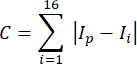
   1. Evaluate the saliency of each candidate keypoint within a node using Equation:
           (1)
      where I_p is the intensity value of the center pixel in a local neighborhood, and I_i represents the intensity values of its 16 neighboring pixels. The absolute difference |I_p - I_i| measures the local contrast between the center pixel and each neighbor. The sum over all 16 neighbors provides a measure of the overall local contrast or texture strength around the center pixel.
   2. Rank all candidates using a dynamic priority queue sorted by the saliency score. From each valid region, select the candidate with the highest saliency response as the representative feature.
4. Optimize and validate feature selection
   1. Combine all selected features across pyramid levels. Ensure uniform spatial coverage across the image. Store the final feature points and their descriptors using the ORB descriptor extractor, version aligned with OpenCV.
   2. Verify that features are not clustered in a few image areas. Feature points should exhibit uniform spatial distribution, supporting robust tracking. Avoid executing image processing in a physical robot system while in motion. Ensure the camera stream is stable and the workspace is cleared.

4. Pose estimation using EPnP

1. Establish 2D-3D correspondences by selecting at least four matched pairs of 3D map points (in world coordinates) and their corresponding 2D image keypoints. Ensure these correspondences are extracted from valid ORB feature matches obtained in the tracking thread.
2. Solve initial pose with EPnP. Continue until each leaf node contains at most one dominant keypoint , or the region size is below 10 x 10 pixels. Use OpenCV's solvePnP function with the cv::SOLVEPNP_EPNP flag to estimate the camera pose.

5. Fine pose refinement with ICP

1. Perform point cloud sampling as described below.
   1. Downsample the source point cloud to reduce computational load and remove redundant data.
   2. Use uniform sampling to ensure structural features are retained evenly across all directions. If needed, apply voxel grid filtering or random selection based on the input point cloud's density and noise characteristics. Ensure the filtered cloud preserves object contours while reducing total point count by at least 50%.
2. Match corresponding points by constructing a KD-Tree from the destination point cloud to enable efficient nearest neighbor searches. For each point in the down sampled source point cloud, find its closest point in the destination cloud using the KD-Tree. Ensure accuracy in point matching, as this step critically affects registration performance.
3. Estimate the optimal transformation as described below.
   1. Use the matched point pairs to compute a rigid-body transformation matrix, including both rotation and translation.
   2. Compute the optimal rigid transformation between the matched point pairs by minimizing the mean squared error (MSE) through singular value decomposition (SVD) of the cross-covariance matrix, which yields the rotation matrix directly, followed by computation of the translation vector based on the rotated centroids.
4. Apply the computed transformation to the source point cloud and update all point coordinates. Repeat the point matching and transformation estimation process iteratively. Continue iterating until either the registration error falls below a predefined threshold or the maximum number of iterations is reached.

6. Dense point cloud map construction

1. Construct a dense 3D point cloud map to achieve an accurate and detailed representation of indoor environments. Follow the steps (see Figure 4) described below.
2. Extract RGB and depth data from keyframes. Select keyframes based on visual richness and spatial coverage. From each selected keyframe, extract both the RGB image and the corresponding aligned depth map from the RGB-D sensor.
3. Convert image pixels to 3D camera coordinates. For each valid depth pixel, project the 2D pixel into 3D space using the intrinsic camera parameters. This process generates 3D coordinates in the camera coordinate system.
4. Transform camera coordinates into world coordinates. Retrieve the optimized camera pose from ORB-SLAM2 for each keyframe. Use the camera pose to transform the 3D camera coordinates into the world coordinate system, aligning all point clouds in a common global reference.
5. Generate colorized 3D points. For each transformed 3D point, assign the corresponding RGB value from the original image. This results in a colorized point cloud that captures both geometry and appearance.
6. Merge point clouds from all keyframes. Accumulate all transformed and colorized point clouds into a unified global point cloud map. Ensure correct alignment using the camera poses associated with each keyframe.
7. Register and refine the final map using PCL. Use the Point Cloud Library (PCL) to refine the final map. Apply filtering to remove noise and down sampling to improve efficiency. Perform global registration (e.g., using ICP) to fine-tune alignment between point clouds if necessary (see Figure 5).
   NOTE: As shown in Figure 6, the initial point cloud alignment during the dense mapping initialization phase may exhibit transient misalignment due to limited observational data, which rapidly converges as additional viewpoints are incorporated. By controlling the robot to traverse the environment, a complete three-dimensional model can be obtained.

7. Generate an occupancy grid map from VSLAM-derived point clouds

1. Down sample the global dense point cloud. Apply voxel grid filtering using a voxel resolution of 0.05 m to reduce redundancy and define the spatial resolution for grid construction.
2. Project 3D points into a 2D occupancy grid. Project all 3D points onto the horizontal (x-y) plane. Discretize the space into uniform grid cells, each representing a 0.05 m x 0.05 m square in the real world.
3. Estimate occupancy probabilities. Use an inverse sensor model to compute the occupancy probability of each cell based on point density and simulated ray-tracing.
   1. Set the occupied probability threshold to 0.65. Set the free probability threshold to 0.35. Classify grid cells with intermediate values as unknown.
4. Apply obstacle inflation. Inflate the occupied regions by applying a circular kernel with a radius of 0.2 m to account for robot clearance and safety margins.
5. Export the occupancy map. Save the generated occupancy grid map in the Portable GrayMap format, accompanied by a corresponding m.yaml metadata file, to ensure compatibility with ROS-based navigation systems.

8. Improved global path planning strategy (based on RRT algorithm)

1. Initialize the path tree. Set the robot's start position as the root node of the tree. Randomly sample points in the configuration (state) space to explore new areas.
2. Identify the nearest existing node. For each newly sampled random point, calculate the Euclidean distance to all existing nodes. Select the node with the minimum distance as the nearest node to serve as the expansion base.
3. Generate a new node toward the random sample. Create a directional unit vector from the nearest node toward the sampled point. Move a fixed step (initially) along this direction to form a new node and connect it to the tree.
4. Replace fixed step size with an adaptive mechanism. Instead of using a constant step size, dynamically adjust the step length based on the local obstacle density. Use larger steps in open environments to accelerate tree expansion. In cluttered or narrow regions, reduce the step size to improve control and obstacle avoidance.
5. Compute the adaptive step size in real time as described below.
   1. Use sensor data (e.g., LiDAR or depth camera) to estimate the density of obstacles around the current region.
   2. If the number of detected obstacles is low, slightly increase the step size. If obstacles are dense, reduce the step size proportionally to insert more intermediate nodes for safe traversal.
6. Iterate the expansion process. Continue sampling, nearest-node searching, and new-node generation using the adaptive step size.
7. Apply B-spline curves for smoothing. Replace the polyline segments in the RRT path with a continuous B-spline curve to improve smoothness. Select control points along the original RRT path, typically at turning points or key waypoints. Construct a control polygon by connecting these control points in sequence.
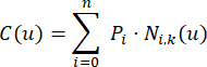
8. Generate the B-spline curve. Use the standard B-spline formula¹⁵:
        (2)
   This formula is used in B-spline curves, where the final curve C(u) is a weighted combination of the control points. The weights are determined by the B-spline basis functions N_i,k (u), which ensure that the curve is smooth and follows the general shape defined by the control points.
9. Set the curve degree to 3 (cubic), which ensures continuity (smooth first and second derivatives). Use the path planning module written in PyCharm 2024.3.

9. Local trajectory optimization with modified TEB

1. Introduce the shortest distance constraint as described below.
   1. To mitigate these drawbacks, integrate a shortest distance constraint into the TEB framework.
   2. Define the constraint as the Euclidean distance between the robot's current position S_t and a future pose S_i+n along the trajectory:
           (3)
      This constraint penalizes inefficient deviations by encouraging the path to stay close to the edge of the global path corridor, improving planning quality and safety.
2. Integrate constraint into TEB cost function by modifying the original TEB optimization graph to include the distance constraint as an additional edge. Adjust the total cost function to include a weighted term for f_os, balancing smoothness, feasibility, and energy efficiency.
3. Integrate constraint into TEB cost function. During optimization, solve for trajectory points that minimize the total cost, including velocity, acceleration, obstacle clearance, and the added shortest-distance term. Use TEB's underlying solver to iteratively optimize the trajectory over N time intervals. Optimize the path considering the constraint (see Figure 7).

Results

Evaluation of improved ORB-SLAM2
Feature extraction experiment
To evaluate the effectiveness of an RGB-D depth camera in practical scenarios, a feature point extraction experiment was conducted. The test was designed using two distinct background environments, each varying in object color and brightness to simulate real-world visual complexity.

Both the proposed improved extraction method and the conventional baseline approach were applied to the same set of test conditions. The number and spatial consistency of the extracted feature points were recorded and analyzed as primary performance indicators.

As shown in Table 1, the number and spatial consistency of the extracted feature points were recorded and analyzed as primary performance indicators. The improved method has increased the percentage of feature points recognized by 25.95%, and the uniformity of feature points has improved by 24.36%. The experimental results, presented in Figure 8, illustrate the comparative performance of both methods. Notably, the improved method yielded a higher number of feature points with enhanced stability across variable lighting and color conditions.

Time-to-completion note: Feature extraction was executed in real time. For each 640 x 480 frame, the complete extraction pipeline (including quadtree filtering and saliency ranking) required approximately 18 ms to 24 ms on a 2.4 GHz quad-core CPU. This allows the system to operate at 40 to 55 FPS, sufficient for real-time SLAM applications.

Experiments on dense point cloud map construction
To address the limitations of sparse point cloud maps in representing continuous scene features and dense obstacle regions, we implemented an enhanced mapping module based on the ORB-SLAM2 framework. Specifically, we incorporated a dense mapping thread to improve environmental perception and navigational robustness in confined indoor spaces.

The mapping experiment was conducted using a differential-drive wheeled mobile robot platform. During operation, the robot navigated a controlled indoor environment while continuously acquiring visual data. The RVIZ visualization tool was used to render real-time mapping output. As illustrated in Figure 9, the green box indicates the current pose of the robot, blue boxes represent the estimated pose of keyframes, and red dots correspond to detected visual features. A complete indoor environment measuring 1.5 m x 6 m was densely reconstructed in approximately 2.5 min to 3 min of runtime. During the process, the system captured approximately 2000-3000 keypoints per frame and accumulated 180-220 keyframes during the reconstruction process. A representative mapping result under well-lit indoor conditions is shown in Figure 10. The red arrow identifies the robot's forward direction at the time of capture. The dense point cloud generated by the proposed method clearly delineates environmental structures, including obstacle contours and spatial geometry.

Compared to conventional sparse mapping, the dense point cloud demonstrates significant improvements in detail fidelity and environmental completeness. This enriched representation supports downstream tasks such as motion planning, obstacle avoidance, and spatial interaction with higher reliability and precision.

Path planning algorithm evaluation
Improved RRT simulation and analysis
To empirically validate the performance of the proposed enhanced RRT-B algorithm, a series of simulation experiments was conducted. The experiment compares four path planning methods: the conventional RRT, the RRT*, the RRT with adaptive step-length and target bias, and the proposed RRT-B, which integrates cubic B-spline smoothing. All algorithms were evaluated within the same simulated environment using 40 independent trials per method. The evaluation of the proposed path planning components was carried out in two complementary stages. Initially, algorithm feasibility and performance were assessed through simulation using the PyCharm development environment. This setup allowed controlled comparisons among baseline and improved methods under consistent environmental parameters. Subsequently, the algorithms were integrated into a full SLAM-based navigation system deployed on a mobile robot platform. In this real-world setting, the robot utilized the enhanced ORB-SLAM2 module for mapping and localization while executing path planning and real-time obstacle avoidance based on the proposed RRT-B and TEB algorithms.

The evaluation metrics include total iteration count, path length, number of path nodes, and path planning time. A summary of the simulation setup and parameters is provided in Table 2. Figure 11 presents the visual outcomes of path generation for each algorithm in an identical simulation scenario. In Figure 11A, the standard RRT demonstrates rapid node expansion but results in irregular, unsmoothed paths with high computational cost. Figure 11B shows RRT*, which improves path quality through local rewiring and optimization. Figure 11C visualizes the adaptive RRT, where dynamic step-length adjustment enhances convergence in complex regions while target bias prevents unnecessary expansions.

The proposed RRT-B method, shown in Figure 11D, applies cubic B-spline smoothing to further optimize path continuity, especially at turns. This significantly reduces abrupt path changes and oscillations, making the algorithm more suitable for real-world navigation tasks that demand high maneuverability.

Quantitative results are detailed in Table 3. Compared with conventional RRT, the enhanced RRT-B achieves an 8.14% reduction in path length, an 85.70% reduction in the number of nodes, a 12.10% decrease in effective search range, and a 16.89% decrease in convergence time. When benchmarked against RRT*, RRT-B reduces path length by 11.35%, node count by 76.09%, lessens the search range by 12.28%, and shortens convergence time by 52.32%.

These findings confirm that the proposed enhancements improve path quality and continuity and significantly optimize computational efficiency. The integration of adaptive step-length control, target biasing, and B-spline smoothing allows the RRT-B algorithm to achieve a robust balance between efficiency and path feasibility.

TEB algorithm enhancement and results
This section demonstrates the effectiveness of the enhanced Timed-Elastic Band (TEB) algorithm through a series of simulation experiments. All tests were conducted within the Python 3.9.18 programming environment, executed on Windows 11. The simulations leveraged a 2D environment for robot navigation using the PyCharm-based visualization tool. As shown in Figure 12, the robot is tasked with moving from a defined start point to a target location while dynamically avoiding obstacles represented by black squares. The 2D robot (visualized as a yellow rectangle) starts moving. During navigation, the robot detects nearby obstacles and begins path re-planning. The enhanced TEB algorithm dynamically adjusts the trajectory in real time to avoid collisions, continuously generating new path segments as needed. As the robot progresses, further path adjustments are made to optimize smoothness and maintain obstacle clearance. The system actively responds to evolving environmental inputs, refining the trajectory accordingly. The robot successfully completes its navigation task, reaching the goal while avoiding all obstacles. The resultant path remains smooth, and no excessive detours or sudden stops are observed, indicating the robustness of the obstacle avoidance mechanism.

Throughout the simulation, the robot demonstrates effective local planning and dynamic obstacle avoidance. The enhanced TEB framework enables real-time reactivity, allowing the robot to adapt its path based on environmental changes. This validates the proposed method's capability to ensure safe, efficient navigation in the presence of unknown, dynamic obstacles.

The velocity profiles of the robot during path planning in a dynamic environment are illustrated in Figure 13. In the initial stage, the robot rapidly accelerates to a steady linear velocity of approximately 0.04 m/s, indicating a relatively unobstructed path. Between approximately 2 s and 7 s, fluctuations in linear velocity and significant variations in angular velocity are observed, suggesting that the robot detected dynamic obstacles and executed deceleration and obstacle avoidance maneuvers. After 7 s, the linear velocity stabilizes and the angular velocity approaches zero, indicating that the robot successfully avoided the obstacles and resumed uniform linear motion. In the final stage, a sharp decrease in velocity and changes in angular velocity suggest that the robot reached its target and autonomously came to a stop, marking the end of the task.

Indoor mapping in real environments
To evaluate the effectiveness of the proposed enhanced mapping strategy, an experiment was conducted in a standard indoor office environment, as shown in Figure 14. The experimental site measures approximately 6 m in length and 1.5 m in width, replicating a typical narrow and confined space common in indoor robotics applications. The full mapping process of the 9 m² test area took approximately 5.8 min, including feature extraction: 1.5 min; keyframe insertion and pose estimation: 2.1 min; dense map reconstruction: 2.2 min. All computations ran onboard in real time at 5 fps for RGB-D input.

The mapping performance of the enhanced ORB-SLAM2 algorithm was benchmarked against the conventional ORB-SLAM2. Evaluation metrics included map completeness, detail fidelity, and the continuity of extracted feature structures.

Prior to the operation, network communication was established by manually modifying the configuration file to assign a static IP address to the host. Once connected, the robot was remotely operated through the host keyboard to execute the mapping sequence. To ensure mapping stability and accuracy, the following guidelines were strictly followed during experimentation: maintain a consistent and moderate robot speed to avoid tracking failure due to motion blur; perform multiple short loop closures to counteract cumulative drift and enhance loop detection frequency; avoid frequent in-place rotations or long stationary pauses, which may lead to visual tracking loss or pose estimation errors.

The robot incrementally constructed the map of the office environment. The mapping process is visualized in Figure 15, showing the robot's trajectory and progressive environmental reconstruction. Figure 16A depicts the final map created using the conventional ORB-SLAM2 method, after the robot navigated the entire space at a steady pace. Notably, distortion and false structures can be observed in the lower-left region. These do not correspond to any actual obstacles and reflect typical inaccuracies also observed during prior Gazebo simulations. Figure 16B presents the output from the proposed improved mapping method. The visualization uses color-coded symbols for clarity: black outlines represent environmental boundaries, black patches denote detected obstacles, such as chairs, and the white square marks the robot's real-time position.

The comparison shows that the enhanced approach substantially improves spatial representation and accuracy. By eliminating the phantom structures found in the traditional method, it provides a map that more faithfully reconstructs the true geometry of the environment. This results in a more reliable base for downstream tasks such as localization, navigation, and obstacle avoidance.

Autonomous navigation performance analysis
This section evaluates the proposed navigation framework with respect to two primary objectives: path planning assessment and trajectory execution verification. The experiments are conducted on the preconstructed environmental map using the enhanced ORB-SLAM2 method. A specific target point is designated on the map, and the robot is instructed to navigate autonomously from its current position toward the target. Both global and local trajectories are continuously monitored and visualized.

The first test case involves selecting a target position located near the robot's starting location. As shown in Figure 17, the green trajectory denotes the global path, calculated by the global planner using the occupancy grid map. The red trajectory indicates the local path, which is dynamically adjusted in real-time based on the proximity to obstacles and other constraints. The curvature observed in the local path near environmental boundaries highlights the robot's obstacle-avoidance capabilities. This interaction between local and global path planning modules ensures both safety and efficiency during navigation.

Figure 18 presents the robot's initial and final positions for this test. There is negligible positional deviation observed at the start and end points, demonstrating accurate pose estimation and smooth execution. No visible jitter, oscillation, or trajectory deviation was recorded. These results validate the system's reliability and high-precision path-tracking performance in close-range navigation scenarios.

In the second test case, the target point is placed at a significantly farther distance from the robot's initial location. Based on the spatial layout, the Euclidean distance between the initial and target positions is approximately 3.62 m, which qualifies as long-distance navigation within the tested scenario. The results are visualized in Figure 19A, where the red trajectory represents the global path generated by the global planner, and the green trajectory indicates the local path continuously adjusted by the local planner in response to environmental dynamics. Figure 19A shows that the path overlaps between the global and local paths are minimal in areas with dense environmental complexity. These regions contain dynamic obstacles, variable terrain constraints, and collision risks. The robot continually adapts its local path to account for these real-time changes, as reflected in the frequent trajectory updates along the path.

In contrast, as depicted in Figure 19B, regions with sparse obstacle distribution show strong alignment between the global and local paths. This suggests that in less cluttered environments, the robot can efficiently follow the pre-planned global trajectory without frequent re-routing. This capability significantly reduces computational overhead and promotes faster navigation through wide-open spaces.

Overall, the results demonstrate that the proposed path planning and execution framework enables robust, real-time navigation. It adapts effectively to both dynamic and static conditions while preserving safety margins and optimizing execution efficiency. The combination of global-local path coordination, dynamic obstacle avoidance, and precise path tracking renders this method suitable for a broad range of real-world indoor robotic navigation applications.

Figure 1: Schematic diagram of a differential drive robot platform in ROS. This figure presents in detail the complete system architecture of a differential drive robot implemented under the framework of the Robot Operating System (ROS). Please click here to view a larger version of this figure.

Figure 2: Quadtree feature point extraction. This figure demonstrates the algorithm process of adaptively partitioning the input image using a Quadtree data structure to efficiently extract and uniformly distribute feature keypoints. Please click here to view a larger version of this figure.

Figure 3: Keyboard layout for manual robot control during mapping the robot. This figure clearly labels the specific key layout on a keyboard used for the teleoperation of a robot, facilitating its movement to assist in environmental mapping tasks. Typically, arrow keys are used to control forward, backward, and rotational movements, and may include additional function keys for starting/stopping the mapping process or saving the map. Please click here to view a larger version of this figure.

Figure 4: Dense mapping thread flow diagram. This figure depicts the complete workflow of the dedicated thread for dense point cloud map generation, presented in a flowchart format. Please click here to view a larger version of this figure.

Figure 5: Flow chart of the ICP algorithm. Using a standard flowchart, this figure elaborates the core procedures and iterative cycle of the Iterative Closest Point (ICP) algorithm for point cloud registration. Please click here to view a larger version of this figure.

Figure 6: Initial position mapping effect when starting dense point cloud mapping. This figure demonstrates the initial mapping outcome upon algorithm activation: successful processing and integration of the first few sensor data frames captured from the robot's initial pose. Please click here to view a larger version of this figure.

Figure 7: Constraint relationship graph of the improved TEB planner. This figure visually represents, via a graph model, the complex interrelationships between multiple constraints in the optimization problem of the enhanced Timed Elastic Band (TEB) planner. These constraints collectively define trajectory feasibility, safety, and smoothness. The optimization involves adjusting a sequence of Path Point states (S_i, S_j) to generate a feasible and optimal trajectory (f_path). Key factors considered include the distance to obstacles (f_dis), the temporal information (T_i) associated with each point, and the overall objective to maintain a safe distance from any Obstacle (f_ob). Please click here to view a larger version of this figure.

Figure 8: Comparison of feature point extraction before and after improvement. (A) Traditional algorithms; (B) Optimized algorithms. A side-by-side comparison visually highlights the improved algorithm's superior performance in feature point distribution uniformity, reduced clustering, and stable feature count. Please click here to view a larger version of this figure.

Figure 9: Visualization of the RVIZ mapping process. This figure displays the real-time mapping monitoring interface within RVIZ, the standard ROS visualization tool. Please click here to view a larger version of this figure.

Figure 10: Dense point cloud map. This figure presents the final high-resolution, high-precision 3D dense point cloud map generated by the algorithm, which accurately reconstructs the experimental environment's geometry with rich detail for subsequent navigation, obstacle avoidance, and 3D reconstruction tasks. Please click here to view a larger version of this figure.

Figure 11: Comparison of path planning results of different algorithms. (A) Traditional RRT algorithms; (B) RRT-Star algorithm; (C) Improved RRT algorithm; (D) B-spline path smoothing. This figure illustrates the complete path optimization process: from the initial RRT-generated path, through RRT* optimization and improved RRT refinement, to the final smooth, safe, and executable trajectory after B-spline smoothing. Please click here to view a larger version of this figure.

Figure 12: Dynamic obstacle avoidance process of the improved TEB algorithm. (A) time = 4s; (B) time = 8s; (C) time = 12s; (D) End. The figure shows how the robot (typically represented as an arrow) dynamically replans its local trajectory based on predicted obstacle motion, smoothly and safely circumventing obstacles before returning to the original global path. Please click here to view a larger version of this figure.

Figure 13: Linear and angular velocity profiles during obstacle avoidance in dynamic environments. This figure quantitatively displays, using time-velocity curves, the continuous variation of robot control commands (linear velocity v and angular velocity ω) during the dynamic obstacle avoidance process shown in Figure 12. The curves reflect control strategies for smooth avoidance, requiring continuity without abrupt changes to ensure stability and comfort. Please click here to view a larger version of this figure.

Figure 14: Environment of the office. This figure is a real-world photograph of an office environment, showing the actual physical setting where mapping and navigation experiments were conducted, including workstations, desks, chairs, and pathways. Please click here to view a larger version of this figure.

Figure 15: Schematic diagram of ORB-SLAM2 office map. This figure is a schematic representation of an office map generated by the ORB-SLAM2 system, typically containing not only point clouds or feature maps but also keyframes with their covisibility relationships or pose graph, representing the map's structure and optimization connections. Please click here to view a larger version of this figure.

Figure 16: ORB-SLAM2 map construction. (A) Traditional ORB-SLAM2 mapping; (B) Improved ORB-SLAM2 mapping. This figure demonstrates the performance differences in mapping before and after algorithm improvements, typically reflected in map completeness (reduced gaps), accuracy (reduced drift), and robustness (performance in low-texture areas). Please click here to view a larger version of this figure.

Figure 17: Robot navigation experiment. (A) Initial position; (B) Location of the target point. This figure indicates the start point of the robot's global path planning task and the target point set by the user via the human-machine interface within the map. Please click here to view a larger version of this figure.

Figure 18: Schematic diagram of the robot's position. (A) Schematic diagram of the starting point of the robot. (B) Schematic diagram of the end point of the robot. Presented in schematic or map annotation form, this figure precisely displays the coordinate positions of the start (A) and end (B) points for the robot navigation task, along with the robot's orientation (pose) at these locations. Please click here to view a larger version of this figure.

Figure 19: Schematic diagram of long-distance navigation of the robot. (A) Schematic diagram of the initial location path. (B) Schematic diagram of the path of the movement process. This figure demonstrates the path planning status for the robot's long-distance navigation task. Please click here to view a larger version of this figure.

Discussion

The two key technologies in autonomous interior navigation systems for wheeled mobile robots that are the focus of this study are visual simultaneous localization and mapping (SLAM)^16,17and path planning¹⁸. The SLAM module proposes a quadtree-based hierarchical selection method to correct the uneven feature point distribution of ORB-SLAM2. To enhance the precision of the generated map, an asynchronous dense mapping approach is employed. The experimental findings demonstrate that the proposed method significantly enhances localization stability and mapping precision, resulting in a 25.95% improvement in feature point extraction accuracy.

In order to surmount the delayed convergence and suboptimal smoothness in path planning that is characteristic of the conventional Rapidly-Exploring Random Tree (RRT) method¹⁹, a novel sampling technique has been developed that integrates goal deviation and adaptive step size. A cubic B-spline function is also employed for trajectory optimization, and the Timed-Elastic-Band (TEB) technique is utilized to facilitate obstacle avoidance in dynamic scenarios. In comparison to the traditional RRT technique, experiments demonstrate that the proposed method effectively enhances trajectory quality and planning efficiency, leading to an improvement of 8.15% in runtime, an 85.70% decrease in node count, and a 12.11% reduction in path length.

However, some limitations remain. The system may underperform in low-texture or poorly lit environments, where fewer features are detected. Dense mapping also introduces computational overhead, which may affect real-time performance on low-end hardware. While current tests were conducted in a 6 m  1.5 m office space, larger environments (>1 m) may present new challenges such as increased pose drift and reduced localization accuracy. Future improvements may include integrating IMU data for more robust tracking or applying submap-based mapping and loop closure strategies to enhance scalability and global consistency. For troubleshooting, mapping drift or phantom structures often indicate camera calibration or RGB-depth misalignment issues, which can be resolved by recalibration. Navigation instability is typically caused by outdated costmaps or poor localization; restarting the planner and ensuring timely map updates can help maintain stable operation.

The validity of the proposed autonomous navigation system is substantiated through a synthesis of simulation and real-world trials, indicating its feasibility for utilization in intricate interior environments for engineering applications. The system demonstrates particular applicability in structured indoor settings with moderate obstacle density and stable lighting conditions, such as office corridors, laboratory spaces, and residential environments.

Materials

List of materials used in this article

Name	Company	Catalog Number	Comments
Astra Pro Plus 3D Camera	CRBBEC	None	3D Camera
TARKBOT-R20-TWD	None	None	ROS Robot

References

Loading...
$$\rightleftharpoonup{xx}$$ $$\longleftharp{xx}$$, $$\longrightharp{xx}$$,
1. VINS-Mono: a robust and versatile monocular visual-inertial state estimator. IEEE T Robot. 34 (4), 1004-1020 (2018).">Qin, T., Li, P., Shen, S. VINS-Mono: a robust and versatile monocular visual-inertial state estimator. IEEE T Robot. 34 (4), 1004-1020 (2018).
2. ORB-SLAM3: an accurate open-source library for visual, visual-inertial and multi-map SLAM. IEEE T Robot. 37 (6), 1874-1890 (2021).">Campos, C., Elvira, R., Rodríguez, J. J. G., Montiel, J. M. M., Tardós, J. D. ORB-SLAM3: an accurate open-source library for visual, visual-inertial and multi-map SLAM. IEEE T Robot. 37 (6), 1874-1890 (2021).
3. SuperPoint: self-supervised interest point detection and description. DeTone, D., Malisiewicz, T., Rabinovich, A. Proc IEEE Conf Comp Vision Pattern Recognit Workshops, , 224-236 (2018).
4. SuperGlue: learning feature matching with graph neural networks. Sarlin, P. E., DeTone, D., Malisiewicz, T., Rabinovich, A. Proc IEEE/CVF Conf Comp Vision Pattern Recognit, , 4938-4947 (2020).
5. BundleFusion: real-time globally consistent 3D reconstruction using on-the-fly surface reintegration. ACM T Graphic. 36 (4), 1(2017).">Dai, A., Nießner, M., Zollhöfer, M., Izadi, S., Theobalt, C. BundleFusion: real-time globally consistent 3D reconstruction using on-the-fly surface reintegration. ACM T Graphic. 36 (4), 1(2017).
6. LaValle, S. M. Technical Report No. 98-11. Rapidly-exploring random trees: a new tool for path planning. , Iowa State University. (1998).
7. Sampling-based algorithms for optimal motion planning. Int J Robot Res. 30 (7), 846-894 (2011).">Karaman, S., Frazzoli, E. Sampling-based algorithms for optimal motion planning. Int J Robot Res. 30 (7), 846-894 (2011).
8. Integrated online trajectory planning and optimization in distinctive topologies. Robot Auton Syst. 88, 142-153 (2017).">Rösmann, C., Hoffmann, F., Bertram, T. Integrated online trajectory planning and optimization in distinctive topologies. Robot Auton Syst. 88, 142-153 (2017).
9. The dynamic window approach to collision avoidance. IEEE Robot Autom Mag. 4 (1), 23-33 (1997).">Fox, D., Burgard, W., Thrun, S. The dynamic window approach to collision avoidance. IEEE Robot Autom Mag. 4 (1), 23-33 (1997).
10. Semantic-aware informative path planning for autonomous exploration with micro aerial vehicles. IEEE T Robot. 38 (5), 3122-3138 (2022).">Chen, Y., Zhong, L., Liu, S. Semantic-aware informative path planning for autonomous exploration with micro aerial vehicles. IEEE T Robot. 38 (5), 3122-3138 (2022).
11. 5G-enhanced visual-inertial SLAM for robust localization in GNSS-denied environments. IEEE T Intell Transp Syst. 24 (6), 6421-6435 (2023).">Kabiri, M., Vos, H., Atia, M. M. 5G-enhanced visual-inertial SLAM for robust localization in GNSS-denied environments. IEEE T Intell Transp Syst. 24 (6), 6421-6435 (2023).
12. FAST-LIO2: fast direct LiDAR-inertial odometry. IEEE T Robot. 37 (4), 1150-1166 (2021).">Xu, W., Zhang, F. FAST-LIO2: fast direct LiDAR-inertial odometry. IEEE T Robot. 37 (4), 1150-1166 (2021).
13. Informed sampling for motion planning in dynamic environments. Int J Robot Res. 41 (5), 517-540 (2022).">Gammell, J. D., Barfoot, T. D. Informed sampling for motion planning in dynamic environments. Int J Robot Res. 41 (5), 517-540 (2022).
14. Variable probability sampling for motion planning in narrow passages. IEEE Robot Autom Lett. 8 (2), 1024-1031 (2023).">Coleman, D., Srinivasa, S. S. Variable probability sampling for motion planning in narrow passages. IEEE Robot Autom Lett. 8 (2), 1024-1031 (2023).
15. The NURBS Book. Piegl, L., Tiller, W. , 2nd ed, Springer-Verlag. (1997).">The NURBS Book. Piegl, L., Tiller, W. , 2nd ed, Springer-Verlag. (1997).
16. Simultaneous localization and mapping: part I. IEEE Robot Autom Mag. 13 (2), 99-110 (2006).">Durrant-Whyte, H., Bailey, T. Simultaneous localization and mapping: part I. IEEE Robot Autom Mag. 13 (2), 99-110 (2006).
17. Simultaneous localization and mapping: part II. IEEE Robot Autom Mag. 13 (3), 108-117 (2006).">Bailey, T., Durrant-Whyte, H. Simultaneous localization and mapping: part II. IEEE Robot Autom Mag. 13 (3), 108-117 (2006).
18. Hybrid motion planning for mobile robots using enhanced RRT and dynamic window approach. IEEE T Robot. 39 (2), 1123-1137 (2023).">Zhang, L., Wang, X., Yang, J. Hybrid motion planning for mobile robots using enhanced RRT and dynamic window approach. IEEE T Robot. 39 (2), 1123-1137 (2023).
19. RRT-connect: an efficient approach to single-query path planning. Kuffner, J. J., LaValle, S. M. Proc IEEE Int Conf Robotics Automat, 2, 995-1001 (2000).
Reprints and Permissions
Request permission to reuse the text or figures of this JoVE article
Request Permission
Tags
Feature MatchingPoint Cloud ReconstructionRapidly Exploring Random TreeTimed Elastic BandPose OptimizationRobot Operating System
Related Articles