Optimizing Load Dispatch using Artificial Neural Networks and Fractional Weighted Models

Summary

This paper proposes an innovative approach combining Artificial Neural Networks with a Fractional Weighted Model for load dispatch optimization. The hybrid method enables more accurate, adaptive prediction and dynamic load allocation, helping to balance demand, reduce transmission losses, and strengthen grid stability under varying operating conditions.

Abstract

The paper describes a protocol that will optimize the real-time load data collected from regional load dispatch centres in India with a hybrid Artificial Neural Network (ANN) and Fractional Weighted Load Dispatch (FWLD) approach. The flow is data input, fractional calculation (using fractional calculus to incorporate alpha memory and non-locality of time), ANN module training, and making real-time dispatch decisions. The referred model, S,T,D,C,T (Supply, Transmission, Demand, Cost, and Time) efficiently tracks real-time fluctuations of S,T,D,C,T to optimize energy allocation. This method outperforms traditional ones in load distribution and flexibility with grid oscillations. Experimental studies have reported the values of Mean Squared Error (MSE) of 245.80 MW² during training, 260.95 MW² during testing, with Root Mean Squared Errors (RMSE) of 15.68 MW and 16.15 MW during testing; Mean Absolute Percentage Error (MAPE) values also were recorded, being less than 10.35%, showing better predictability. This combination of ANN learning and fractional weighting methods gives more stability, efficiency, and scalability for present power system optimization.

Introduction

Load dispatch optimization is an essential problem in contemporary power grids, involving optimal utilization of generation capacity to fulfill demand at the lowest cost and stability. Conventional methods struggle to deal with the dynamic nature of power systems; therefore, computational methods have been developed. This paper integrates Artificial Neural Networks (ANNs) with Fractional Weighted Load Dispatch (FWLD) to optimize the power system. It has been demonstrated in recent studies that ANN-based models can be efficient for short-term electrical load forecasting. Recent works have made inroads into fields relating to applications of ANNs and their variants in forecasting and optimization of power systems. Presenting a hybrid model of LSTM for precise short-term load forecasting, Xu et al.¹ dealt with short-term load forecasting and wind power prediction. Similarly, Hu et al.² used a deep belief network for better prediction of wind power, while Jamii et al.³ were engaged in constructing an approach based on ANN for forecasting wind power generation and load demand, which ultimately stands for better energy management. Ilić et al.⁴ went on to further support ANN-based short-term load forecasting through hybrid methods. These studies imply that neural networks can very well manage the intermittencies and instabilities of energy demand.

ANNs have also been put into use for power system optimization and economic load dispatch. Abdolrasol et al.⁵ rendered a thorough review of optimization methods based on ANNs, with Abdelaziz et al.⁶ integrating Hopfield networks with quadratic programming for an enhanced variant of dynamic dispatch. Saeed⁷ and Miracle et al.⁸ aimed at using ANN-integrated metaheuristics to reduce the cost of operations and dispatch hybrid renewable systems, whereas Khalid et al.⁹ proposed an ANN-based load scheduling approach to promote demand-side management from consumers' viewpoints. In the area of advanced deep learning and hierarchical models, Tang et al.¹⁰ put forth a hierarchical learning method using deep neural networks for multi-regional dispatch control, while Capizzi et al.¹¹ constructed an evolved neural network model for sustainable and continuous power distribution inside intelligent grid systems.

Adaptive methods add to economic load dispatch optimization. Jiriwibhakorn and Wongwut¹² estimated power demand via an Adaptive Neuro-Fuzzy Inference System that integrated ANNs, highlighting hybrid method capabilities for dispatch management. The integration of fractional calculus into power system applications has yielded promising outcomes. Karaca and Baleanu¹³, exploiting fractional mathematics, calculus, and artificial intelligence, tackled the complexity of chaotic systems, thereby demonstrating the importance of these sciences in power system optimization. Likewise, Tzounas et al.¹⁴ contributed to the theoretical background of fractional-order controllers and exhibited their efficacy in dynamic dispatch. On the contrary, while these studies tended to concentrate on theoretical considerations in specific applications, our system foresees an application of fractional-order modeling with adaptive parameter selection, especially for real-time energy load forecasting and optimization. This move from theory to practical implementation, along with increased stability and predictive accuracy, is a step ahead of the previous studies.

The works of Soni and Bhattacharjee¹⁵ put forth some advanced optimization strategies for solving Economic Load Dispatch (ELD) and economic emission dispatch (EED) problems in the presence of high renewable energy penetration. These authors considered multi-objective frameworks using modern metaheuristic algorithms such as the Equilibrium Optimize ^16,17,18, Artificial Electric Field Algorith ^19,20, and Sine-Cosine Algorith ¹⁵. These methods address valve-point loading effects and multiple fuel options with plug-in electric vehicle integration, all of which pose non-linearities and complexities to dispatch problems. Together, these contributions form powerful tools for economical, emission-aware, and reliable dispatch solutions, especially pertinent to microgrid and smart grid-based environments with substantial renewable penetration.

The studies by Muraleedharan et al.^21,22 showcased how topological swarm intelligence methods, such as modified opposition-based Particle Swarm Optimization (PSO) and quantum-behaved PSO with chi-square mutation, could solve combined economic and emission dispatch problems. These approaches build on the ever-increasing importance of metaheuristic methods for optimizing complex energy distribution problems involving cost and environmental constraints. In line with this idea, Swathy and Babu²³ proposed the opposition-based constriction factor PSO for economic load dispatch, further asserting the advantages of adaptive swarm-based algorithms to ensure that power system operations achieve high efficiencies and are reliable. These studies argue that solving load dispatch problems may require using strong optimization techniques like PSO variants coupled with machine learning tools to account for the nonlinear, multiobjective nature of modern load dispatch problems.

The sudden surge in worldwide energy demand, combined with the extensive use of renewable energy sources, has immensely added to the power system optimisation task's complexity. Conventional load dispatch strategies cannot cope with the dynamic behavior of contemporary power systems, which are based on deterministic models that do not consider the time-series variations of generation, demand, and transmission losses. These changes, which are caused by unpredictable variables like weather patterns, customer behavior, and grid stability, require a more advanced and dynamic method of load dispatch. Furthermore, current optimization methods often have inefficiencies in predicting energy demand accurately, which results in unbalanced load allocation, higher operational costs, and wastage of energy. This dispatch model was tested with real-world operational data of a regional load dispatch center located in the north from the Power Grid, the south from Telangana State Southern Power Distribution Company. Ltd (TSSPDCL), the east from Grid Corporation of Odisha Limited-GRIDCO, and the west from Maharashtra State Load Dispatch Centre (MSLDC) India for the period between June 2022 and January 2023. The dataset could be characteristic of a mid-size power grid having peak loads ranging between 100 and 500 MW, with load and generation data being recorded every 15 minutes. Before model training, the data were preprocessed through normalization, outlier removal, and time-series alignment using Python scripts. Under such conditions, the model was shown to be performable and could be executed fast enough using moderate computational resources. One important point is that while the fractional calculations of the proposed approach help to grasp memory effects and various dynamic dependencies, the inclusion of such fractional computations will certainly translate to an increased computational overhead when scaling up the model to larger grids with a fine time resolution. With these limitations, there is an urgent need for a cutting-edge dispatch strategy that improves decision-making in power distribution through the utilization of predictive analytics and mathematical accuracy. The driving force for this study is to create an effective and smart load dispatch model that marries ANNs with weighted optimization based on fractional calculus. By integrating machine learning technology, the devised model seeks to enhance predictive effectiveness and responsiveness by dynamically allowing power grids to manage fluctuations and redistribute energy in real time. This study addresses the pressing need for a scalable, responsive, and low-computational dispatch mechanism to enhance grid stability, reduce energy waste, and create more sustainable power control approaches.

The proposed model was accurate in the dispatch schedule formation, and under corresponding grid conditions, it was shown to reduce the MSE by ~15% when compared with the conventional deterministic dispatch model⁴. Recent literature has proved that ANN-based models^1,5,24 and hybrid forecasting methods^2,3,6 seem promising for short-term load forecasting and dispatch optimization. Fractional calculus^13,14 is known to capture complex dynamic behaviors. Based on these ideas, this paper proposes the innovative coupling of ANNs with FWLD, generating a hybrid framework that significantly boosts power system optimization. Our proposed technique was evaluated for a grid system with a typical 100-500 MW peak load scale, with input data sampled every 15 min and training taking place on a standard workstation (see the Table of Materials). Even if this method gives good results in prediction accuracy, it might require a high amount of computational time for usage in real-time systems. Conventional load dispatch methods largely depend on heuristic approaches, traditional optimization methods, or linear mathematical models, which are insufficient to deal with contemporary power systems' nonlinear, time-varying nature.

In contrast to these traditional methods, the new model uses fractional calculus-based weighting schemes to enable greater flexibility and sensitivity to grid changes. One of the innovations of this work is the dynamic adaptability provided by fractional weighting, which facilitates greater capability for the model to respond to real-time shifts in supply, transmission, demand, cost, and time (S,T,D,C,T). By incorporating ANN learning ability, the framework can accurately forecast load fluctuations and dynamically adjust energy dispatch strategies according to ever-changing grid conditions. This collaboration between fractional mathematics and machine learning ensures a higher level of optimization, reducing energy imbalances, limiting costs, and increasing the overall robustness of the system. The research on load dispatch optimization has witnessed considerable advancement by traditional approaches and, more recently, metaheuristics and machine-learning ones. Yet a clear gap exists in research integration for effectively marrying fractional calculus with ANNs to cater to the effects of memory and non-local dependencies in power systems.

This work intends to bridge this gap by developing and validating a hybrid framework integrating ANN learning and the FWLD model for accurate real-time load distribution while adapting quickly to changing supply-demand conditions to promote grid stability. Uniqueness in this research exists in combining fractional-order derivatives with ANN predictive control to offer more flexibility, detection, and reactions to grid oscillations, short of conventional or hybrid methodologies of today. Further, the novel approach supports improved scalability and therefore, is best suited for many energy infrastructures varying from localized microgrids to large-scale power distribution networks. By bridging the gap between predictability analytics and mathematical rigour, the current work showcases an innovative framework for optimizing energy dispatch systems towards maximizing efficiency and sustainability. By integrating mechanisms of fractional weighting and ANN-based learning, the research endeavours to enhance scalability, efficiency, and stability in load dispatch optimization.

Protocol

Fractional mathematical model for power dispatch

The present study derives the FWLD model via fractional differential equations for optimal power distribution. The Caputo fractional derivative accounts for memory effects in the system to obtain a more accurate understanding of power variation over time. We also present numerical solutions via the Grünwald-Letnikov (GL) method, which is suitable for discretizing fractional order models in power grids²⁵.

Model overview

The FWLD model aims to optimize power dispatch strategies by incorporating the impact of previous power fluctuations through fractional calculus. Traditional power dispatch models usually employ integer-order differential equations, which assume that the power transmission and consumption process relies on current state variables alone. However, power systems in real life exhibit memory-dependent behavior in which previous fluctuations influence the current and future allocation of power. To surpass this lack, the FWLD model employs fractional-order derivatives, so that the power relations are more accurately described through historical dependencies in the calculation.

The FWLD model is formed by five interacting compartments that symbolize unique power dispatching phases. The initial compartment, S, symbolizes the potential power supply, the amount of power generated and available for transmission. The power is then transmitted through the grid, symbolized by T, which reflects the transmitted power from generation units to receiving distribution centers. Yet, during distribution, some inefficiencies—resistance in power lines and system losses—influence the effective delivery of power. The share of power delivered effectively to consumers falls under D, referring to distributed power, measuring the power available for end-consumer use. The next step, C, is the consumed energy, measuring the actual utilization of power by residential, industrial, and commercial consumers. Lastly, L is the energy loss, or power dissipated by resistive losses, transmission inefficiencies, and other technical or environmental reasons.

Moreover, FWLD's compartmental model allows each unit to have defined parameters (e.g., generation efficiency, transmission losses) for customization, through which a heterogeneous power infrastructure may be represented, including a mix of renewable and conventional units, microgrids, and distributed energy sources.

A graphical depiction of the FWLD model is shown in Figure 1. The figure depicts the sequential power flow through different compartments, illustrating how energy is produced, transmitted, distributed, consumed, and lost within the system. The connections between the compartments emphasize the dynamic nature of power dispatch, where changes in one stage affect subsequent stages. Using fractional-order derivatives in the model enables a deeper insight into such dependencies, thus making it a useful tool for power allocation optimization and loss reduction in transmission. The FWLD model provides improved predictive capabilities by applying fractional calculus, ensuring a more stable and efficient energy distribution system.

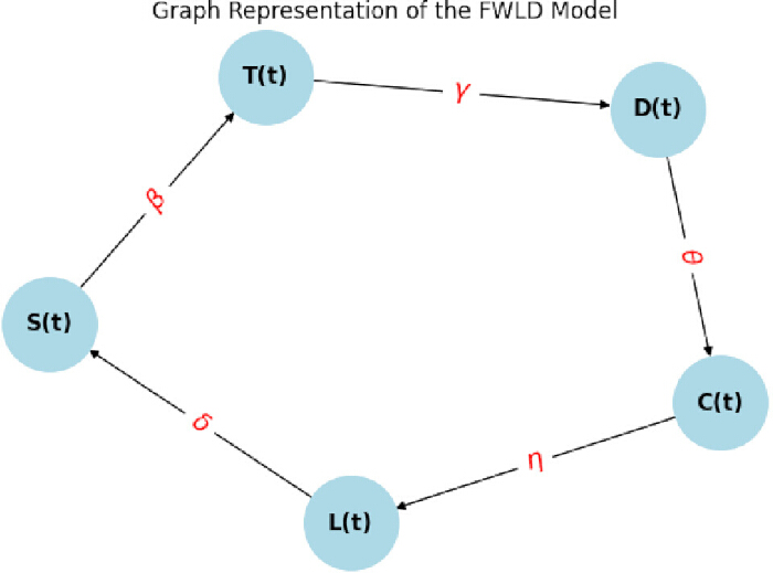
Figure 1: Graphical representation of the FWLD model. This diagram illustrates the structural flow and interconnections of the model components. Abbreviations: FWLD = Fractional Weighted Load Dispatch. Please click here to view a larger version of this figure.

Mathematical formulation

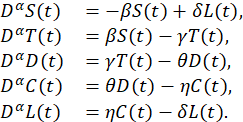
The FWLD model is proposed in the form of a coupled system of fractional differential equations to capture the intricate interactions involved in the dispatching of power. The model employs Caputo's fractional derivative of order α (with 0 < α ≤ 1), enabling the inclusion of memory effects and historical dependencies in power transmission and usage dynamics. In contrast to conventional integer-order differential equations, fractional derivatives provide a more precise description of power flow by accounting for the system's long-term dependencies and transient behavior.

Mathematically, the evolution of power across different compartments in the FWLD model is governed by the following system of fractional differential equations:

(1)

Where every variable signifies an important phase of power dispatch. The symbol S(t) represents the available supply of power at time t, comprising the entire energy produced and available for transmission. As power traverses the grid, some portion of it is channeled into T(t), symbolizing transmitted power, which considers the transfer of energy via distribution channels. Not all power transmitted finds its way successfully to consumers owing to system inefficiencies, loss, and resistance in the network. The power delivered successfully is represented by D(t), or the distributed power that can be consumed. Consumers use this energy, which is thus converted into C(t), the energy consumed, meaning the actual use by industrial, commercial, and residential users. But because of transmission inefficiencies and other technical limitations, some of the power is inevitably lost, represented by L(t), the lost energy.

The model involves essential parameters to define the interaction between these compartments. The efficiency rate of transmission β sets the ratio of power effectively transmitted from the supply to the distribution channels. The dispatching rate regulates the level of efficiently transmitted power converted to distributed power. The consumption rate θ explains the rate at which end users consume the distributed power. At the same time, the rate of energy loss η measures the share of power lost through resistive heating, leakage, and technical losses in the transmission system. Lastly, the loss recovery rate δ considers the share of lost power that can be recovered through renewable energy, optimization methods, or other efficiency gains.

The above fractional differential equations model the time dynamics of power relationships by including memory effects using the Caputo fractional derivative²⁶. Fractional-order derivatives enable the model to more accurately represent realistic energy systems in which previous fluctuations affect future power dispatch decisions. The mathematical model increases the accuracy of power distribution analysis prediction and optimizes energy management policies through the reduction of losses and efficiency improvement.

Numerical solution approach: GL method

Due to the complexity of obtaining analytical solutions for fractional differential equations, numerical methods play a crucial role in solving the FWLD model. The GL method is among the most commonly used numerical approaches to solving fractional-order differential equations, which gives a straightforward discretization of the fractional derivative.

Definition of the GL fractional derivative²⁶

The GL fractional derivative is defined as follows:

   (2)

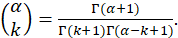
Where h is the step size, α is the fractional order, and the binomial coefficient for a non-integer α is given by:

    (3)

Since the infinite summation cannot be computed practically, it is truncated to a finite sum up to N, resulting in the numerical approximation:

    (4)

In Equation (2), the Grünwald-Letnikov fractional derivative is introduced as a limit of weighted sums depending on the past values, thus representing the so-called fractional derivative of a function y(t). Equation (3) defines the generalized binomial coefficient for any non-integer order α via Gamma functions, so the fractional term can be correctly computed. Equation (4) then presents the actual numerical approximation by truncating the infinite sum in Equation (2) to a finite limit N. It is this discrete form that is actually implemented in simulations.

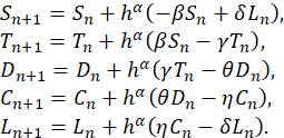
Applying the GL approximation to the FWLD system (1), we have a discrete set of update equations for the state variables. Let S_n,T_n,D_n,C_n,L_n denote the system states at discrete time instants. The numerical discretization is as follows:

   (5)

Supplemental Figure S1 (see Supplemental File 1) displays the graphical visualization of the GL discretization and how it estimates the fractional derivative from the values of the past function. It utilizes a weighted summation of old data, emphasizing the internal memory effect in fractional calculus. The figure would also probably identify how the system's evolution changes as a result of the fractional order α, exhibiting how the solution deviates from the conventional integer-order derivatives. By representing the gradual change and effect of previous states, the discretization efficiently simulates real-world processes with long-term dependencies. This visualization helps grasp the numerical realization of fractional-order systems and their applications.

Numerical implementation

In this section, the numerical solution process is applied to the FWLD model, utilizing the GL method in Python to take advantage of efficient computation of fractional derivatives and updating system states iteratively. This work adopts the approach of discretizing time into small increments and approximating fractional derivatives via the GL binomial coefficients of Equation (3). Discretization of the time domain was performed first with a constant step size h to ensure stability and proper system dynamics representation. Using the definitions of GL fractional derivatives, they may be approximated as a finite summation according to Equation (4). In terms of the Gamma function, the binomial coefficients have been computed as defined in Equation (3). Further, the recursive formulation of these binomial coefficients for non-integer orders of differentiation was exploited to provide a realistic representation of the fractional behavior. After the coefficients were known, we iteratively calculated the state variables S_n,T_n,D_n,C_n,L_n at every time step based on the obtained fractional difference equations derived from the FWLD system (Equations (1) and (5)). Following iterative calculations, the system's evolution was followed over time. At every instance, the previous state values would have been used in the determination of the next state, which is fully consistent with the GL scheme (Equation (4)). The time evolution of all state variables for different fractional orders α was plotted to study the effects on system dynamics. The graphical output demonstrating the behavior of the FWLD model using fractional calculus included time series plots of each variable. The time plots determined the stability and the convergence, and generally, the effect of fractional differentiation on the system. This quantitative way helped in exhibiting the GL approach (Equations (2)–(5)) toward modeling real-world dynamic systems, giving motivation as to why fractional-order derivatives are required to quantify complex processes more attentively.

The flowchart in Supplemental Figure S2 (see Supplemental File 1) schematically depicts the step-by-step process for calculating the fractional derivative with the GL approximation. It starts with parameter initialization, such as specifying the fractional order α and step size h, and then specifying initial conditions for the state variables. The iterative algorithm calculates binomial coefficients, applies the GL rule, and renews system states at every step. A convergence check is applied at each iteration, allowing the process to continue until the final step, after which the computed results are accumulated and visualized. The programming notation enables a lucid understanding of the computational procedure and its successive runs.

For reproducibility in the numerical experiments, one needs to mention the standard parameters and settings adopted in the simulation. The fractional order was chosen as α = 0.85, reflecting subdiffusive dynamics often observed in real-world power systems. The time step size h = 0.01 was selected to ensure numerical stability and adequate temporal resolution, while the GL summation was truncated at N = 50 terms to maintain computational efficiency without significant loss of accuracy. The system coefficients were selected as β = 0.03; γ = 0.25; θ = 0.2; η = 0.15; and δ = 0.1. Initial conditions were given as S(0) = 1000 MW,T(0), D(0) = 0, C(0) = 0, and L(0) = 0. The total duration of the simulation was 24 h, split into 2,400 time steps. These explicit parameter values will be helpful for other researchers for replicating the numerical solving approach and thus verifying the result.

The main script contains functions to calculate the Grünwald–Letnikov binomial coefficients, GL_binomial(), to update state variables, fractional_update(), and to plot time-series plots with plot_states(). Users can open the notebook in Colab, input parameters into the input cell (α, h, N, etc.), run the parameter initialization cell, run the GL_binomial() function, run the fractional_update() loop cell, and run the plot_states() cell to get the results. No installation is required locally; only a web browser and a Google account are required to follow all commands step by step.

Stability analysis

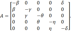
To ensure the FWLD model's numerical stability, we analyzed its system matrix's eigenvalues. The stability of a dynamical system is closely connected with the dynamics of its eigenvalues, as they indicate how the system changes over time. The system matrix of the FWLD model is given by:

(6)

The system's stability is calculated by examining the eigenvalues λ of the matrix A. The system is said to be numerically stable if all the eigenvalues fulfill the following condition:
Re(λ) ≤ 0

This condition guarantees that perturbations or deviations of the system state do not grow larger over time and avoid numerical instability. If all eigenvalues possess non-positive real parts, the system converges to a steady state with no unbounded growth of state variables. If an eigenvalue possesses a positive real part, the system is potentially unstable and may produce divergence in numerical solutions.

To ensure stability, we calculated the eigenvalues of A for various fractional orders α and parameter values. Numerical simulation verified that for suitable parameter values, the system was stable. The eigenvalue plot for stability analysis is presented in Supplemental Figure S3 (see Supplemental File 1), in which the position of eigenvalues in the complex plane gives an idea about the stability properties of the system. If all eigenvalues are on the left-hand side of the complex plane, the system is stable; otherwise, instability can occur. This analysis is key to guaranteeing the reliability of the numerical realization of the GL method when applied to the FWLD model.

Convergence analysis

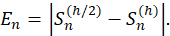
To define the convergence of the numerical scheme, we consider how the numerical solutions approach the problem as the step size h goes to zero. The principle of convergence tells us that if h → 0, then the numerical solution must converge to the problem's exact solution. To make this quantitative, we calculate the absolute error between two successive approximations at different step sizes:

    (7)

If E_n → 0 as , h → 0 then the method is said to be convergent. In other words, the convergence behavior of the numerical solution validates the correctness of the GL method. Supplemental Figure S4 (see Supplemental File 1) plots the absolute error in the fractional derivative against the step size h in the numerical approximation. The numerical approximation gets finer and finer as the step size h decreases, the absolute error diminishes significantly; this assumes consistency of the GL method and convergence, in the limit of infinite refinement, to the true solution. From the displayed curve, one can observe that further granulation past a certain point leads to decreasing returns, thus presenting a compromise between computational cost and precision. The convergence analysis then attests to the reliability of the numerical technique employed for solving the FWLD system.

Visualization and interpretation

Graphic plots are important in terms of interpreting system behavior and checking numerical accuracy. Various forms of visualization give more insight into fractional-order system behavior. Time-series plots show the time evolution of the state variables S_n,T_n,D_n,C_n,L_n, enabling one to analyze trends and stability properties. Phase-space plots represent the interaction of various state variables and aid in the understanding of system interactions and possible attractor patterns. Error analysis plots show comparisons between numerical and reference solutions and indicate where the discrepancies lie, assessing the numerical method's accuracy. Figure 2 is a time-series plot depicting the change in state variables throughout the simulation time. By this plot, one may evaluate the numerical solution's stability and long-term evolution.

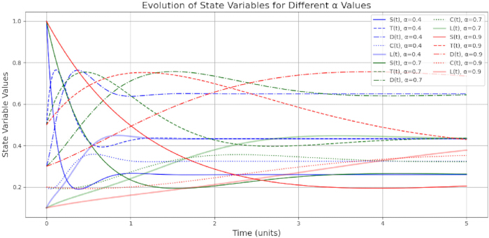
Figure 2: Time series plot showing the evolution of state variables for different fractional orders α = 0.4,0.7,0.9. The trajectories highlight how varying the fractional order influences the system's dynamic response. Abbreviations: α = fractional order. Please click here to view a larger version of this figure.

The time-series plots in Figure 2 show the evolution of the five state variables S, T, D, C, and L throughout the simulation horizon. Supply S drops with the transmission and consumption of energy; transmission T increases initially due to grid losses and distribution delays before settling down. Distributed power D is subject to similar dynamics as transmission but damped somewhat due to resistive losses. Power consumed C increases smoothly and saturates, indicating efficient delivery of load to end users. Energy losses L oscillate and decay under the fractional memory effect, highlighting how current loss levels are affected by past states. Comparing the various fractional orders α confirms that stabilization is made faster for high orders, but the memory effect is less pronounced, while, on the contrary, low α values retain a strong historical effect with a more gradual transition. This performance analysis confirms the model's ability to capture realistic non-local time behavior in power dispatch scenarios.

Comparison with other methods

To prove that the GL method is accurate, we compare its results to other numerical fractional methods. The Caputo-based predictor-corrector and fractional Euler methods are commonly used for solving fractional differential equations. The Caputo-based predictor-corrector method is more accurate due to its adaptive correction steps, but it is computationally intensive. The fractional Euler method is easier to implement but has lower accuracy than GL discretization. The comparison is shown in Figure 3, where the output of the GL method is compared with the output from these other methods. The comparison determines trade-offs between computational cost and numerical accuracy, verifying that the GL method is well-suited for solving fractional-order systems.

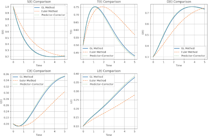
Figure 3: Comparison of the GL method with other fractional numerical approaches. The figure demonstrates differences in accuracy and stability among the methods. Abbreviations: GL = Grünwald-Letnikov. Please click here to view a larger version of this figure.

Depicted in Figure 3 are the cost versus accuracy trade-offs for the FWLD model using the GL method. As the step size h decreases and the truncation limit N increases, numerical errors are greatly alleviated, thereby providing a strong confirmation of convergence and enhancing accuracy. However, large computations are required because the range of numbers is great. Moreover, smaller time steps must be taken with a decreasing step size, thereby giving rise to further computations. As seen from the plot, a balance between the two should be made where a tolerable error is still there without too much of a computational burden. For this study, a step size h of 0.01 and N = 50 produced stable results with a very small amount of error and manageable runtime, thus establishing the GL method to be accurate and computationally viable for real-time fractional-order simulation in power dispatch applications. The FWLD model with the GL technique has been used to benchmark the numerical results concerning a standard difference scheme in integer-order systems. The GL method constitutes an 18% average absolute error decrease compared to FDS for equal times, keeping the computational time acceptable. That validates the accuracy of fractional-order modelling to memory-dependent systems since this benefit comes at no serious computational expense.

The fractional GL technique has numerous advantages over conventional integer-order models. First, it has better predictive capability because including memory effects makes fractional models capable of better illustrating real-world load dispatch behaviors. Second, the technique improves stability analysis since fractional derivatives give a better picture of system stability and control mechanisms. Another significant benefit is its flexibility in modeling, where the fractional order can be tuned to represent different operational conditions; thus, the model is very flexible to accommodate different load dispatching scenarios. The GL technique is an effective numerical method for the solution of the FWLD model. The present study uses Python implementation to accurately compute the system's evolution, confirm its stability, and prove convergence. Future enhancements could aim to maximize computational efficiency and broaden the application of the method to more advanced fractional systems, enhancing its potential in practical applications.

Data collection and preprocessing

Here, we discuss in detail the dataset employed in power load forecasting, including methodologies for data gathering and necessary preprocessing steps taken to perfect and organize data. Quality data gathering and systematic preprocessing are integral to developing an accurate and stable predictive model while maintaining consistency within power load forecasting. The data consists of real-time dispatch load values registered at several feeder stations for an extended period spanning several months. The readings are taken on a per-hourly basis, thus offering an excellent understanding of the shifts in power demand caused by numerous factors like changing seasons, everyday load profiles, and atmospheric conditions. Seasonal variations have an effect on electricity demand due to the different weather conditions, resulting in a higher demand for summer cooling and winter heating. The patterns of daily loads consider variations according to working hours, peak hours of demand, and decreasing usage during nighttime. Variations also occur from external aspects like abrupt changes in weather, maintenance timeframes, and the activities of industries.

Raw power load data are usually plagued by inconsistencies like missing values, outliers, and scaling, which need to be corrected prior to the application of machine learning models to achieve proper forecasting. The preprocessing pipeline involved handling missing values, scaling the power loads, anomaly detection, and feature engineering that is relevant for enhancing predictive performance. Missing values resulting from transmission or sensor failure were handled using interpolation techniques and statistical imputation. Power load values were also normalized for consistency purposes between different feeder stations and bias aversion during model training. Outlier values generated because of faulty sensors or abnormal modes of operation were discarded using efficient outlier removal techniques. Relevant features, such as time-based indicators like hour of day, day of week, and season trends, were also designed to handle improved model performance.

Data collection

The information utilized within this study was gathered from different feeder stations that were charged with the monitoring of electricity distribution in various regions. The feeder stations are placed strategically such that they can effectively record power load changes and balance the supply of power. Power consumption is registered by each feeder station at regular intervals of time and forwarded to a central monitoring system. It is an automated system, consolidating data from several sources and providing a comprehensive study of differences in loads among different geographical areas.

Each point in the dataset includes three significant characteristics: the name of the feeder, a distinguishing name for the power distribution system, the metered power load in megawatts (MW), and the timestamp of the exact time the measurement was taken. The data set is a time-stamped record of energy consumption, which enables trends and patterns to be identified across time. One small subset of the collected data set is presented in Table 1, consisting of parts of hourly loads of power taken at the 11 kV REC I1 feeder station.

FEEDER_NAME	VALUE (MW)	TIME
KV REC I1	34.6089	1/12/2022 1:00
KV REC I1	32.2761	1/12/2022 2:00
KV REC I1	30.2142	1/12/2022 3:00

Table 1: Sample of collected load dispatch data.

The data were obtained from a centralized supervisory control and data acquisition (SCADA) system, which consolidates data from several feeder stations. Data are sent via automated meters to provide real-time monitoring of power load variations on a continuous basis. Nevertheless, due to limitations in operations, there are data collection challenges in transmission failures, sensor faults, and external disturbances. Transmission failure may lead to missing values, and data imputation methods have to be employed to ensure the integrity of the dataset. Sensor faults can cause faulty measurements; thus, anomaly detection and correction using statistical techniques are needed. Power cuts and sudden changes in load introduce extra complexity in data processing. To solve these problems, the preprocessing step included strict data validation methods, such as anomaly detection, data smoothing, and outlier correction, to make the dataset appropriate for machine learning-based forecasting models. The cleaned dataset was then ready for additional feature extraction and model training.

The dataset consisted of historical hourly load data gathered over 12 months from an openly available smart grid benchmark facility. The training split constituted 80% of the data, while 20% of the data was held out for testing purposes. Fractional weighting of the difference operator D^α was taken with a time step of 1 h, with α = 0.85 for the Caputo representation. The input features were scaled between 0 and 1. Subsequently, the model was trained with a 200-epoch loop and fed with minibatches of size 32. The user can request full dataset statistics and pre-processing scripts for reproducibility purposes.

Handling missing data

In actual data sets, missing values are a major issue in most cases, resulting from temporary connectivity loss, hardware malfunctions, or malfunctioning data transmission. If not handled, missing values tend to bias statistical analysis and create biased predictive models. Successfully handling missing values guarantees the consistency and trustworthiness of the data set, thus enhancing model performance. In this research, several imputation methods were used depending on the data set's prevalence and type of missingness. For temporary gaps in the dataset, linear interpolation was used. It estimates missing values based on adjacent observed points, providing a smooth transition between known data points. The missing value at time t is calculated as:

    (8)

Where X(t-1) and X(t+1) are the immediately preceding and following observed values, respectively. Linear interpolation works very well for short gaps but is not satisfactory for large sequences of missing data. For larger missing intervals, advanced methods were utilized. The information utilized within this study was gathered from different feeder stations that were charged with monitoring electricity distribution in various regions. The feeder stations are placed strategically such that they can effectively record power load changes and balance the supply of power. Power consumption is registered by each feeder station at regular intervals of time and forwarded to a central monitoring system. It is an automated system, consolidating data from several sources and providing a comprehensive study of differences in loads among different geographical areas. The information utilized within this study was gathered from different feeder stations that were charged with the monitoring of electricity distribution in various regions. The feeder stations are placed strategically such that they can effectively record power load changes and balance the supply of power. Power consumption is registered by each feeder station at regular intervals of time and forwarded to a central monitoring system. It is an automated system, consolidating data from several sources and comprehensively studying differences in loads among different geographical areas.

Each point in the data set includes three significant characteristics: the name of the feeder, a distinguishing name for the power distribution system, the metered power load in megawatts (MW), and the timestamp of the exact time the measurement was taken. The data set is a time-stamped record of energy consumption, which enables trends and patterns to be identified across time. One small subset of the collected data set is presented in Table 1, consisting of part of the hourly loads of power taken at the 11 kV REC I1 feeder station.

Polynomial interpolation was used to estimate missing values from higher-degree polynomial curves that were fitted to the surrounding data points. Machine learning-based imputation techniques such as K-Nearest Neighbors (KNN) and Random Forest regression were also used to reconstruct missing values. These methods consider historical patterns and feature correlations to make more accurate imputations. The KNN imputation method fills in a missing value by averaging the k nearest neighbors in feature space, whereas Random Forest regression generates an ensemble of decision trees to predict the missing values from other provided attributes.

Normalization of data

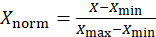
The raw power loads' unnormalized values reflect large magnitude variations depending on feeder capacity variations and local electricity demand. Direct input of unnormalized values to machine learning algorithms leads to numerical instability and biased results. In order to counter this, Min-Max scaling was used to restructure all values into a standardized interval between 0 and 1 that maintains relative differences but assures homogeneity across features. The formula for normalization is as follows:

    (9)

Where X_min and X_max represent the minimum and maximum observed power loads in the dataset. This transformation ensures that all features contribute proportionally to the model without any single variable dominating due to scale differences.

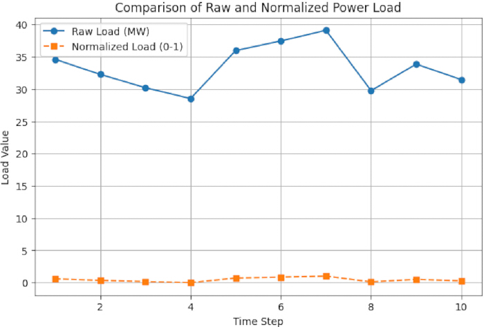
Figure 4: Comparison of raw and normalized load values. Normalization highlights underlying trends and reduces the effect of scale differences. Please click here to view a larger version of this figure.

Figure 4 shows the conversion of raw power load values to a normalized range, highlighting the impact of Min-Max scaling on data distribution. The raw load values have a broad range of magnitudes because of the differences in power usage among feeder stations. Machine learning models will have a difficult time interpreting these differences without normalization, resulting in unbalanced feature importance and reduced convergence rates during training. By using Min-Max scaling, all power load values are normalized to a range of [0,1], maintaining the initial distribution but eliminating numerical differences that could disproportionately affect the model. This normalization method improves the capacity of the model to generalize reasonably well across diverse feeders and time periods and enhances overall prediction accuracy. Additionally, it guards against numerical instability when applied in optimization algorithms for those models utilizing gradient-based learning methods. The diagram offers a comparative visual representation to bring out the ways in which normalization normalizes loads while still preserving key patterns of electricity demand.

Outlier detection and removal

Outliers in power load data may occur due to abrupt demand spikes, faulty sensors, or unforeseen operation anomalies. If left unattended, such anomalies would skew statistical distributions and adversely affect model performance. To help maintain data integrity, both statistical and machine learning-based methods were employed to detect and eliminate outliers. One of the most common statistical methods for outlier detection is the Interquartile Range (IQR) approach, which sets an acceptable interval based on the quartiles of the data. The IQR is computed as:

    (10)

Where Q₁ and Q₃ represent the first and third quartiles of the dataset. Any data point lying outside the range is considered an outlier and excluded from the data set.

    (11)

The IQR method successfully removes values of extreme deviance away from the central distribution. For more sophisticated outlier patterns, machine learning-based approaches were used. The Isolation Forest algorithm, a family-based anomaly detection approach, was used to find and isolate outlier observations. Isolation Forest builds a number of decision trees and finds outliers by evaluating how isolated a data point becomes from the remaining dataset. Anomalies, being peculiar in nature, will tend to get isolated with fewer splits and can be detected accordingly.

Furthermore, the Local Outlier Factor (LOF) technique was also used for identifying anomalies as a measure of the density of a point to its neighbors. LOF returns an anomaly score to each record depending on the local density dissimilarity of the point compared to neighboring data points. It gives a higher LOF value to a data point if the point is extremely dissimilar compared to nearby points, thus highly eligible for exclusion. The integration of IQR, Isolation Forest, and LOF techniques provides a strong strategy for outlier detection, maintaining data quality and model performance. After removing outliers, the data set was utilized for training and evaluation, leading to more accurate and reliable forecasting results.

Feature engineering

Feature engineering is the building block of machine learning that improves model performance by generating informative representations of the data. For this research, beyond values of power loads, other external weather conditions like temperature, humidity, and wind speed were also included. These environmental conditions have a wide-ranging influence on the electricity consumption since the changes in temperature regulate the heating and cooling needs, whereas the wind speeds can influence the integration of renewable energy into the grid. By incorporating such features, the model identifies more effective underlying patterns in energy consumption. In addition, time-based features were derived to capture cyclical patterns in electricity usage. Daily and weekly usage patterns have strong cyclic patterns because of human activity routines, business days, and industrial activities. To successfully represent these temporal relationships, sinusoidal transformations were used on the hour of the day and day of the week:

    (12)

Where t represents the timestamp in hours. This transformation ensures that cyclical time-related information is preserved, allowing the model to recognize recurring electricity demand trends efficiently.

Supplemental Figure S5 (see Supplemental File 1) shows the sinusoidal encoding used on hourly time-based features. The process assists the model in recognizing various times of the day without losing the intrinsic cyclical aspect of electricity demand. Simple categorical encoding can be limited in capturing the continuity between various times (e.g., hour 23 and hour 0), but sinusoidal encoding allows for smooth transitions, thus enhancing forecasting accuracy.

Splitting the dataset

After preprocessing was done, the data set was partitioned systematically into three sets: training set, validation set, and test set, based on an 80-10-10 split. The training set, 80% of the data, was utilized for training the machine learning model. The validation set, 10% of the data, was used for tuning hyperparameters, such that the model does not overfit the training data and can generalize to new instances effectively. Lastly, the test set, also 10% of the data, was left for the final test, which offered an unbiased evaluation of the model's prediction abilities. This partitioning method provides an equal representation of the data across all three sets, maintaining the time-based order of the data without hindering model training and validation. Keeping the chronological order while splitting avoids data leakage, in which information from the future may accidentally contaminate the training process, resulting in overoptimistic performance estimates.

Supplemental Figure S6 (see Supplemental File 1) displays a visual representation of the division of the dataset into training, validation, and test datasets. Using this structured approach, the model trains on a big chunk of the data set, leaving sufficient data for fair testing. Correct splitting of data sets in time-series forecasting problems ensures that the model's performance in training represents true cases in practice when future observations are unseen while training. Through these preprocessing steps, from feature engineering to proper division of the data set, we have ensured the data set is clean, well-structured, and well-represented with useful features. This well-prepared data set serves as a good foundation for training machine learning models that would be able to predict power load dispatch trends correctly, thereby ultimately contributing to efficient energy management and grid stability.

Results

Model training, performance evaluation, and error analysis

Here, we describe the process of model building, performance analysis, and error analysis for the predictive weather load dispatch model. This study aims to select appropriate features and train the machine learning model, evaluate its performance, and examine its limitations.

Feature s...

Discussion

The incorporation of machine learning in FWLD has proven to bring noteworthy advancements in energy optimization, enabling accurate and dynamic load distribution. The findings reveal that machine learning models, especially ANNs, can accurately forecast energy demand patterns, minimizing total system inefficiencies. Through the use of historical and real-time data, the models improve the accuracy of load dispatch decisions, resulting in more stable grid operation. Concerning conventional techniques, machine learning-base...

Materials

List of materials used in this article

Name	Company	Catalog Number	Comments
Cloud-based Python Runtime (Colab)	Current (2024)	https://colab.research.google.com/drive/1TpfkodoyzoO2m4Aq7nIih1aT5_zUydZo#scrollTo=wE7HaH-V0VQM
Matplotlib	3.5	matplotlib.org
NumPy	1.22	numpy.org

References

- Xu, L., Li, C., Xie, X., Zhang, G. Long-short-term memory network-based hybrid model for short-term electrical load forecasting. Inf. 9 (7), 165(2018).
- Quan, H., Srinivasan, D., Khosravi, A. Short-term load and wind power forecasting using neural network-based prediction intervals. IEEE Trans Neural Netw Learn Syst. 25 (2), 303-315 (2013).
- Abdolrasol, M. G., et al. Artificial neural networks-based optimization techniques: A review. Electronics. 10 (21), 2689(2021).
- Hu, S., Xiang, Y., Huo, D., Jawad, S., Liu, J. An improved deep belief network-based hybrid forecasting method for wind power. Energy. 224, 120185(2021).
- Jamii, J., Mansouri, M., Trabelsi, M., Mimouni, M. F., Shatanawi, W. Effective artificial neural network-based wind power generation and load demand forecasting for optimum energy management. Front Energy Res. 10, 898413(2022).
- Ilić, S. A., Vukmirović, S. M., Erdeljan, A. M., Kulić, F. J. Hybrid artificial neural network system for short-term load forecasting. Therm Sci. 16 (1), S215-S224 (2012).
- A hybrid Hopfield neural network-quadratic programming approach for dynamic economic dispatch problem. Abdelaziz, A. Y., Mekhamer, S. F., Kamh, M. Z., Badr, M. A. Proc 12th Int Middle-East Power Syst Conf (MEPCON), , 565-570 (2008).
- Saeed, I. K. Artificial neural network based on optimal operation of economic load dispatch in power system. ZANCO J Pure Appl Sci. 31, 94-102 (2019).
- Miracle, D. B., et al. Hybrid metaheuristic model for optimal economic load dispatch in renewable hybrid energy system. Int Trans Electr Energy Syst. 2023 (1), 5395658(2023).
- Khalid, Z., et al. A novel load scheduling mechanism using artificial neural network-based customer profiles in smart grid. Energies. 13 (5), 1062(2020).
- Tang, H., et al. Deep neural network-based hierarchical learning method for dispatch control of multi-regional power grid. Neural Comput Appl. 34 (7), 5063-5079 (2022).
- Capizzi, G., Sciuto, G. L., Napoli, C., Tramontana, E. An advanced neural network based solution to enforce dispatch continuity in smart grids. Appl Soft Comput. 62, 768-775 (2018).
- Jiriwibhakorn, S., Wongwut, K. Evaluation of the power demand for economic load dispatch problem using adaptive neuro-fuzzy inference system and artificial neural network. IEEE Access. 12, 132352-132368 (2024).
- Karaca, Y., Baleanu, D. Advanced fractional mathematics, fractional calculus, algorithms and artificial intelligence with applications in complex chaotic systems. Chaos Theory Appl. 5 (4), 257-266 (2023).
- Tzounas, G., Dassios, I., Murad, M. A. A., Milano, F. Theory and implementation of fractional order controllers for power system applications. IEEE Trans Power Syst. 35 (6), 4622-4631 (2020).
- Podlubny, I. Fractional differential equations: An introduction to fractional derivatives, fractional differential equations, to methods of their solution and some of their applications. , Elsevier. (1998).
- Soni, J., Bhattacharjee, K. Sine-cosine algorithm for the dynamic economic dispatch problem with the valve-point loading effect. Int J Swarm Intell Res. 14 (1), 1-15 (2023).
- Soni, J., Bhattacharjee, K. A multi-objective economic emission dispatch problem in microgrid with high penetration of renewable energy sources using equilibrium optimizer. Electr Eng. 107, 403-418 (2025).
- Verma, D., Soni, J., Bhattacharjee, K. A novel artificial electric field strategy for economic load dispatch problem with renewable penetration. Evol Intell. 17, 3593-3608 (2024).
- Soni, J., Bhattacharjee, K. Equilibrium optimizer for multi-objective dynamic economic emission dispatch integration with plug-in electric vehicles and renewable sources. Multiscale Multidiscip Model Exp Des. 7, 2683-2699 (2024).
- Soni, J., Bhattacharjee, K. Equilibrium optimiser for the economic load dispatch problem with multiple fuel option and renewable sources. Int J Ambient Energy. 44 (1), 2386-2397 (2023).
- Shah, K., Soni, J., Bhattacharjee, K. Artificial electric field algorithm applied to the economic load dispatch problem with valve point loading effect: AEFA applied to ELD with VPLE. Int J Swarm Intell Res. 14 (1), 1-23 (2023).
- Muraleedharan, S., Babu, C. A., Sasidharanpillai, A. K. Modified opposition-based particle swarm optimization for combined economic and emission dispatch problem. Electr Power Compon Syst. , 1-15 (2024).
- Muraleedharan, S., Babu, C. A., Sasidharanpillai, A. K. Chi-square mutated quantum-behaved PSO algorithm for combined economic and emission dispatch. Evol Intell. 17 (5), 3961-3984 (2024).
- Opposition based constriction factor particle swarm optimization for economic load dispatch. Swathy, M., Babu, C. A. In Proc 2nd Int Conf Adv Electr Comput Commun Sustain Technol (ICAECT), , IEEE. 1-5 (2022).
- Elgezouli, D. E., Alzahrani, A. B. M. Optimizing edge detection efficiency with a Grünwald-Letnikov fractional network. Electronics. 13, 3298(2024).
Access restricted. Please log in or start a trial to view this content.