Rapid in-silico Battery Electrolyte Electrochemical Reaction Generation using 3T-VASP Multi-Scale Energy Minimization

Summary

The 3T-VASP framework combines hierarchical structure transformation with ab initio multi-scale gradients to significantly reduce the number of steps needed to escape local energy minima and model electrochemical reactions. This protocol presents a method for generating electrochemical reaction byproducts for various electrolyte component combinations using only 100-150 static DFT calculations.

Abstract

Electrolytes are important components in lithium-ion batteries. However, battery degradation due to irreversible electrochemical reactions in the electrolyte can consume electrolyte molecules and severely reduce its effective operation lifetime. It is hence important to study the electrochemical reaction pathways in the battery electrolyte to further improve lithium-ion battery reliability. Unfortunately, it is difficult to experimentally study the exact electrolyte electrochemical reaction pathways in the electrolyte, which usually contains many chemical species (different solvents, salts, additive molecules, and electrode interfaces). These reaction byproducts may form complex solid electrolyte interphase (SEI) on the electrolyte-electrode interface (LiF, Li₂CO₃, Li₂O, LiOH, organolithium compounds, etc), which are more difficult to analyze, instead of being released as the easier-to-analyze small gas molecules. Our recent publication on the tiered tensor transform technique in combination with density functional theory software (tiered tensor transform- Vienna Ab-initio Simulation Package (VASP), or 3T-VASP) enables the practical usage of the ab-initio approach to generate physically meaningful electrolyte electrochemical reaction byproducts within just 100-150 DFT steps. In this work, we describe the inner workings of the 3T-VASP code (publicly available on Github) in greater detail, along with the simulation preparation steps needed to correctly set up the 3T-VASP workflow for new electrolyte systems of interest beyond the examples presented in the original 3T-VASP publication.

Introduction

Investigation of electrochemical reaction pathways in new battery electrolyte compositions is important for identifying methods to improve electric vehicle battery performance and lifetime¹. However, such studies are often difficult because battery electrolytes are often made by mixing different components, such as solvent, salt, and additive molecules, which interact with themselves and with different surfaces (cathode and anode electrodes) under different battery operating voltages and temperatures². In experiments, some of the irreversible electrolyte electrochemical decomposition reactions are easier to investigate because they produce small gas molecule byproducts which are released from the electrolyte solution into the air (correspondingly making it easier to probe using experimental techniques such as gas chromatography^3,4,5). However, many of these byproducts are larger molecules or complex organic-inorganic solid mixtures, such as complex organolithium polymer compounds⁶, which will not be released into the environment as gas molecules. This makes it difficult to study these more complex electrochemical reaction pathways experimentally².

Ab-initio modeling, such as density functional theory (DFT), is a promising method to study potential electrochemical degradation pathways in the electrolyte in silico⁷. However, simple DFT energy minimization of complex electrolyte structure (liquid mixture with experimentally reasonable electrolyte component concentrations in a periodic boundary condition box) will mostly fail to generate low-energy structures corresponding to physically meaningful electrochemical reaction byproducts. The DFT-minimized structures typically have higher energy and represent non-physical byproducts that correspond to incorrect electrochemical degradation pathways, because the structures are trapped in local energy minimums during the DFT energy minimization procedure. Methods such as ab-initio molecular dynamics (AIMD)^8,9, neural network force field^{10,11,12,13,14,15,16}, or DFT-based metadynamics^17,18,19 are often used to explore more diverse electrolyte structures, which may include more meaningful electrochemical reaction byproducts. Computational screening to generate electrolyte components that are predicted to be electrochemically more stable is also often attempted²⁰. However, all these methods have their own drawbacks, such as: requiring large and lengthy computational resources⁷, large amount of ab-initio training data¹³ or prior knowledge about the eventual electrochemical reaction byproducts to bias the simulation into specific results²¹.

We have recently introduced a method to perform ab-initio structure energy minimization in a multi-scale manner by connecting the energy gradients obtained from any ab-initio method, such as DFT atomic forces calculated using Vienna Ab-initio Simulation Package (VASP) software²², with the structure transformation function gradients calculated using PyTorch (3T-VASP)^23,24. This approach enables the user to simply set up a simulation box filled with multiple types and counts of electrolyte component molecules and run an external atomic energy and force calculator (such as a classical force field or VASP DFT). The structure energy minimization is then automatically performed in a multi-scale manner, which respects the natural structure transformation modes of the relevant molecules (translations and rotations of different segments of the molecule). Because a 3T-VASP simulation is typically 'completed' within 100-150 static DFT calls while generating physically meaningful reaction byproducts (many of these were experimentally observed in prior literature)²⁴, it is possible to run many different ensembles of 3T-VASP trajectories to generate potentially meaningful electrochemical reaction pathways and byproducts in the electrolyte for further computational or experimental investigation. The principles and math behind the multi-scale gradient structure minimization have been discussed in depth in a prior publication²⁴. In this work, we aim to further detail the 3T-VASP software architecture and computational workflow, the setup of the computing environment necessary to run 3T-VASP, the preparation of input files for 3T-VASP simulation of new systems, the monitoring of 3T-VASP simulations, and the example of output trajectories.

First, it is necessary to understand the overall architecture of the 3T-VASP software, as shown in Figure 1. 3T-VASP works by identifying and exploiting the natural structure transformation modes in the molecule (because these are structure transformations that are easier for the molecules to perform while maintaining relatively low ab-initio structure energy)²⁴. While it is possible to manually program these structure transformation modes for each new molecule species (it is cumbersome to do so), 3T-VASP offers to automate this process for the user by exploiting the information available in the classical force field file representing the molecule²⁴. Once these structure transformation modes are determined for the desired electrolyte molecule components, the user needs to specify the periodic boundary condition box and its lattice vector parameters (the box may originally be empty, or partially filled with individual cations or electrode surface) to be further filled with desired types and numbers of other electrolyte molecules (such as solvents, salt ions, additives). The 3T algorithm will then use either classical force field (a built-in classical force field calculator is included with 3T-VASP) or the computing environment's VASP software to calculate atomic energy and forces to perform multi-scale structure transformation, which can minimize the structure energy in a modest number of static DFT calls²⁴. This computational cost reduction makes it possible to repeat the electrochemical reaction trajectory and byproduct generation for large number of initial structures.

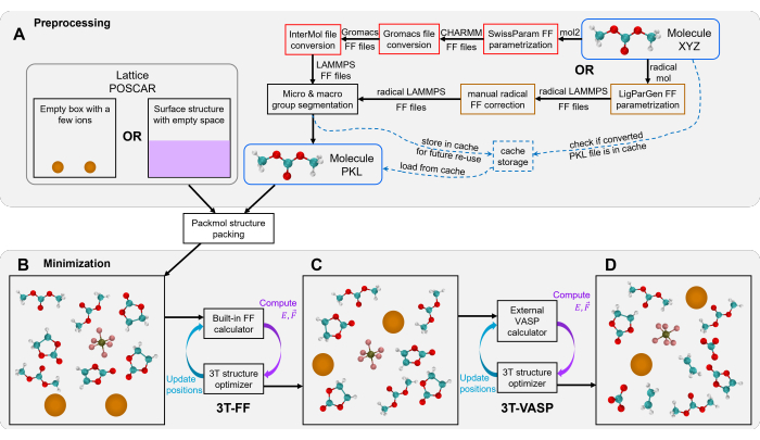
Figure 1: Computational workflow of 3T-VASP. (A) Preprocessing of 3T-VASP input structures (periodic boundary condition lattice and small molecules). The small molecule force field parametrization can be done either automatically using SwissParam webserver, manually modified after LigParGen webserver parametrization, or loaded from a cache based on previously finished parametrization. The micro and macro group segmentation of 3T algorithm is done automatically by parsing the molecule substructures based on their rotatable bonds. The PBC lattice input file is in the format of VASP POSCAR file and should be designed to have enough empty physical space to pack the desired number of input molecules. The PBC lattice can be an empty box filled with a few ions or a surface structure with some empty space. (B) The desired types and numbers of small molecules are put into the empty space in the PBC lattice using PackMol. (C) Multi-scale gradient 3T structure minimization using built-in force field calculator (3T-FF, mostly to enable liquid dispersion and create a physically reasonable initial structure for 3T-VASP without allowing for chemical reactions). (D) Multi-scale gradient 3T structure minimization using external software such as the VASP calculator (3T-VASP enables electrochemical reactions to proceed). Please click here to view a larger version of this figure.

Various open-source external software, such as GROningen Machine for Chemical Simulations (GROMACS), a classical force field-based molecular dynamics software, which is useful for running large-scale molecular dynamics simulations²⁵ and InterMol, a Python library codebase developed by Shirts et al. for molecular dynamics file format conversions²⁶, are utilized to enable automated molecule force field parametrization and rotatable bond extraction. VASP is used to enable electrochemical reaction during the ab initio phase (3T-VASP cycles). The steps needed to install these dependencies are presented in this article.

Protocol

1. Setting up a computing environment for running 3T-VASP

NOTE: It is recommended to use Linux²⁷ for the following steps.

1. Set up the conda environment²⁸ dedicated to running 3T-VASP.
   1. Install conda (such as miniconda) on the Linux machine by following the official instructions (refer to the Table of Materials for the link).
   2. Create a new 3T conda environment, activate it, and install git by running the following commands:
      conda create --name 3T python=3.11
      conda activate 3T
      conda install git -c conda-forge
   3. Clone the 3T-VASP github repository and enter the directory
      git clone https://github.com/jpmailoa/External_3T.git
      cd External_3T
   4. Install mamba to manage conda dependencies, and install the required libraries for the 3T conda environment:
      conda install mamba -c conda-forge
      mamba install --file requirements.txt -c pytorch -c conda-forge -c rdkit
2. Install the software GROMACS in the 3T environment.
   1. Install GROMACS in the 3T conda environment (the installation instructions can be found in Table of Materials).
      NOTE: If the user does not plan to process any new molecule into a .pkl format (see step 2.3) and can work with existing molecules that have been previously processed (in the form of .pkl file), this GROMACS installation (step 1.2) may be skipped.
3. Install the modified version of InterMol in the 3T environment.
   1. Follow these instructions to install a bugfix version of InterMol:
      cd utils/Convert_Gromacs_LAMMPS/InterMol
      python setup.py build
      python setup.py install
      cd ../../..
      NOTE: If the user does not plan to process any new molecule into a .pkl format (see step 2.3) and can work with existing molecules which have been previously processed (in the form of .pkl file), this InterMol installation (step 1.3) may be skipped.
4. Specify VASP software path in 3T-VASP code.
   1. Install the VASP software on the 3T environment. The instructions and tutorials can be found in Table of Materials.
   2. Open the file 'utils/calculator_3T_VASP.py' and check the 'run_VASP' function. Look for the following default line in the Python script:
      os.system('nohup mpirun -n '+n_gpu+' --allow-run-as-root ~/software/vasp.6.2.1/bin/vasp_std')
      1. The above default line should be modified to the OS system call which points to the user's VASP executable and specifies the computing resources, for example:
         os.system('mpirun -np 2 /path/to/vasp/bin/vasp_std')
5. Ensure that necessary non-Python third-party libraries are available in the 3T conda environment by running these commands in the Linux terminal (or install if necessary):
   gmx
   wget
   unzip
   packmol
   NOTE: These commands will only be called during the molecule force field format file pre-processing, so if the user is only planning to work with pre-processed molecule .pkl files, the 'wget' and 'unzip' libraries do not need to be installed.
6. Perform a test run to ensure that 3T-VASP has been configured correctly.
   1. Use Python to run either of the following test scripts, which are provided based on a prior publication²⁴:
      python randomize_3T_bulk_electrolyte_reduction.py
      ​python randomize_3T_bulk_electrolyte_oxidation.py
   2. A successful execution will generate logs in the output file 'default.log', which can be monitored in a separate Linux terminal (example shown in Figure 2).

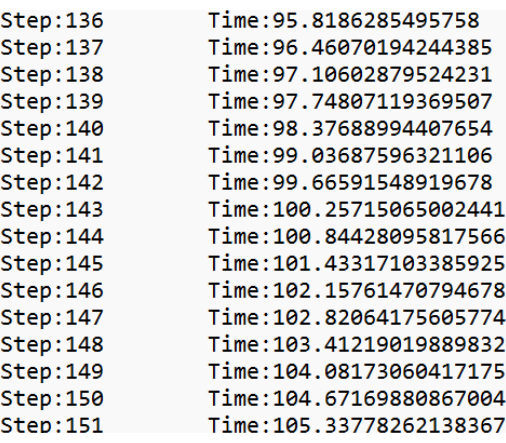
Figure 2: Example content of a 3T logfile during a test run after a successful installation. The default logfile simply logs the current step number of a 3T cycle and the computing time that has elapsed since the beginning of the cycle. Please click here to view a larger version of this figure.

2. Preparing 3T-VASP input files

1. Prepare periodic box lattice structure in VASP POSCAR file format.
   1. Name the 3T-VASP lattice files as '.vasp' and save them in a subfolder of the 'input' folder (such as 'input/Electrolyte_Reduction' folder). Write the files in the format of a VASP POSCAR file. An example of such PBC lattice POSCAR file with three lithium cations inside it is shown below in Figure 3.
2. Prepare periodic box lattice structure property override file.
   1. Name these 3T-VASP lattice structure property override files as '.override', place them in the subfolder of the 'input' folder (such as 'input/Electrolyte_Reduction' folder from step 2.1), and write them in the JSON format as a dictionary with the key entry 'movable_group' and 'atom_charge_proximity' (see example in Figure 4).
3. Prepare molecule structure files in the XYZ file format.
   1. Name these 3T-VASP molecule structure files as '.xyz' (see example in Figure 5) and place them in the 'input' folder. 3T-VASP will check whether the '.xyz' has previously been converted into a .pkl file or not, and if not, the molecule will be processed using a free external third party SwissParam force field parametrization webserver²⁹. If force field parametrization is based on another webserver such as LigParGen³⁰ or manual parametrization is desired, please refer to step 2.6.
4. Prepare template VASP input files to be used during each 3T-VASP step.
   1. Use the standard VASP input files such as INCAR, KPOINTS, and POTCAR (POSCAR not needed). In the INCAR file, ensure that the number of steps in molecular dynamics runs NSW is either not set or set to the default value of NSW = 0 (example shown in Figure 6). Place these files in a subfolder of 'templates/VASP' folder (such as 'templates/VASP/Electrolyte_Reduction').
5. Prepare a 3T config file that configures all the other input files.
   NOTE: This config file should be provided in the form of a JSON list format (with each member of the list being a dictionary block which indicates the settings of one 3T cycle)²⁴ and placed in the 'configs' folder (such as 'configs/Electrolyte_Reduction.json', example shown in Figure 7 below). Unspecified parameters in each cycle will inherit the parameters from the configuration of the previous cycle.
6. (Optional) If needed, use manual parametrization or LigParGen webserver to parametrize the molecule force field.
   1. Use LigParGen or manual parametrization for molecules that cannot be parametrized by SwissParam, such as charged molecules, resonant structures, or radicals. Refer to the additional examples provided for guidance:
      python example_LigParGen_FF_assignment.py
      python example_manual_FF_assignment.py

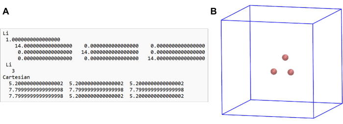
Figure 3: Example of PBC lattice POSCAR file filled with a few lithium ions. (A) The box size is 14 × 14 × 14 ų, and there is sufficient empty space to be subsequently packed by electrolyte molecules using PackMol. (B) The PBC lattice file, which is essentially a VASP POSCAR file that can be directly visualized using third-party software such as Visual Molecular Dynamics (VMD)³¹. Please click here to view a larger version of this figure.

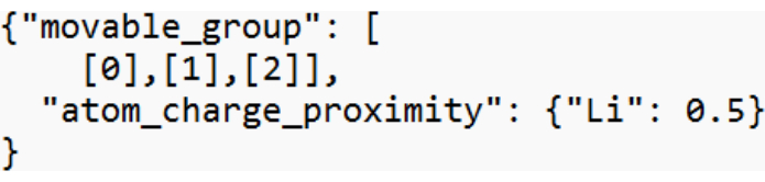
Figure 4: Example of PBC lattice property override file. This dictionary describes the property modifications which should be applied on atoms inside the PBC lattice. The example nested list entry for the key ‘movable_group’ means that Lithium atom 0,1,2 are all individual groups of atoms which can move independently during the 3T simulation. In addition to that, partial charge value of +0.5 are applied on each Lithium atom using the key ‘atom_charge_proximity’. Please click here to view a larger version of this figure.

Figure 5: Example of a molecule XYZ file. (A) This file is in the format of a standard molecule XYZ file containing just the atom elements and coordinates. (B) This molecule XYZ file can be directly visualized using third-party software such as VMD. Please click here to view a larger version of this figure.

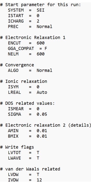
Figure 6: Example of an acceptable 3T template VASP INCAR file. Most settings in this file should be tuned based on the user's needs. The only requirement for 3T-VASP relaxation is that NSW value is either not set or set to NSW = 0. Please click here to view a larger version of this figure.

Figure 7: Example of 3T config file. Each element in the list (a block) represents the settings of a 3T cycle ('mode' determines whether the cycle is a 3T-FF or a 3T-VASP minimization). When a key is not specified in a block's dictionary, it means the key-value pair from the previous block will be used instead. 'lattice_poscar' specifies the location of VASP-style lattice structure POSCAR file ('file', step 2.1) and its override file ('override', step 2.2, if any is available). 'molecule_xyz' specifies all the additional molecule species we would like to add into the PBC box, with 'file' specifying the molecule XYZ file location and 'count' specifying the number of such molecule species to be added into the PBC box. 'mode' specifies either 'FF' (3T-FF mode) or 'VASP' (3T-VASP mode). 'n_epoch' specifies the number of minimization steps which should be done in that 3T cycle. 'out_tag' specifies the name which should be used for that cycle's associated log files (and hence the user should give the cycles unique names to prevent accidentally overwriting important log or output files). 'print_freq' specifies how frequently the output log file should be written to (1 = output to log file on each step). When 3T-VASP mode starts being used, the user should further specify the folder location of the VASP template files in the 'VASP_template' key of the 'lattice_poscar' dictionary. Please click here to view a larger version of this figure.

3. Run 3T-FF and 3T-VASP energy minimizations

1. Perform single 3T-FF/3T-VASP trajectory generation.
   1. For an example config file from step 2.5 ('configs/Electrolyte_Reduction.json'), run the commands:
      python
      >> from main_run_utils import main
      >> main('configs/Electrolyte_Reduction.json')
      NOTE: Depending on the user's machine configuration, it may take several hours to finish this trajectory generation (it contains 250 VASP DFT static calls). The user may track the progress by inspecting the content of the 'default.log' file in a separate Linux terminal (step 1.6).
2. If large-scale trajectory generation is desired, prepare a Python script to automate config file generation and utilization.
   1. For the large-scale automation script (Figure 8), write a short function (such as 'config_modify_func') to replace specific phrases in the config template file (such as 'configs/Electrolyte_Reduction_template.json'). This will automatically generate new config files to produce different 3T-VASP trajectories. For example, run the following large-scale automation script:
      python randomize_3T_bulk_electrolyte_reduction.py
      NOTE: Once the 3T-VASP code has been set up correctly and the simulation has been started, the 3T multi-scale structure minimization will run in the background. Depending on the user's machine configuration, it may take several days to finish the generation of multiple trajectories. This protocol example contains 2500 VASP DFT static calls (10 3T-VASP trajectories), which will be finished within 30-40 h on a compute node with 4 Nvidia V100 GPUs. As mentioned in step 3.1.1, the overall progress can be tracked by checking the content of the 'default.log' file in a separate Linux terminal. 3T-VASP will also periodically dump the output trajectory, which can be reviewed in real time. In the config file example (Figure 7, step 2.5), the 'out_tag' field in a 3T block describes the name of the output files where the results from that 3T cycle will be written. For example, 'out_tag' value of 'FF_step3' means that the entire cycle's atomic trajectory will be written onto 'FF_step3.xyz' (in the form of multi-frame XYZ file format) while the energy calculated by the built-in 3T force field calculator of the 'FF' mode (or DFT energy calculated by VASP in the 'VASP' mode) will be written onto 'FF_step3_outE.txt' (the energy unit in this file is in Kilocalorie per mole [kcal/mol]).

Figure 8: Example of 3T-VASP trajectory generation automation script. A template config file needs to be provided as the 'tag' input to the 'multiple_runs' function. In addition to that, the number of trajectories to be generated (10) and the function that modifies the content of the template config file to generate new random config files (the 'config_modify_func' function) also need to be provided. Please click here to view a larger version of this figure.

Results

If the 3T energy minimization is set up correctly, one should observe a gradual dispersion of electrolyte molecules inside the PBC box during the 3T-FF phase, without any chemical reaction happening (Figure 9A). It is important to note that 3T-FF relies on classical force field energy, so it is necessary that the force field parameters are good enough to ensure that molecules maintain their correct geometries and that the 3T trajectory neither collapses (inter-species attraction too strong) ...

Discussion

The main advantage of the 3T algorithm is its ability to enable fast structure energy minimization, which can easily escape trivial local energy minimums by performing the structure minimization in a hierarchical manner through multi-scale tensor gradient backpropagation. Because of this, the 3T optimizer tends to generate physical low-energy structures in complex systems, which are harder to optimize using other structure energy minimization algorithms²⁴. While the structure transformation and gr...

Materials

List of materials used in this article

Name	Company	Catalog Number	Comments
Conda	Conda		The official instructions to install Conda on the Linux machine can be found in: https://docs.conda.io/projects/conda/en/stable/user-guide/install/linux.html
GROMACS software	Biophysical Chemistry Department, University of Groningen	2021.3	Gromacs executable release from August 18, 2021. Standard executable in the newest version should work as well, although not tested yet. The installation instructions for GROMACS in the 3T conda environment can be found in this link: https://manual.gromacs.org/documentation/2021.3/download.html and https://manual.gromacs.org/2021.3/install-guide/index.html
InterMol software	Shirts Group, University of Colorado Boulder	External_3T version	The original InterMol code developed by Shirts group has a bug associated with Gromacs -> LAMMPS force field conversion. The InterMol version included in External_3T Github distribution is required to fix this bug.
JoVE article input files	Tencent Quantum Laboratory		Input file examples for this JoVE manuscript available from the 3T-VASP Github page at https://www.github.com/jpmailoa/External_3T
JoVE article scripts	Tencent Quantum Laboratory		Python scripts for this JoVE manuscript available from the 3T-VASP Github page at https://www.github.com/jpmailoa/External_3T
VASP software	Computational Material Physics, Dept. of Physics, University of Vienna	vasp.6.2.1	VASP executable release from May 17, 2021. Standard parallel VASP executable in the newest version should work as well, although not tested yet. Instructions and tutorials for VASP can be found in these links: https://www.vasp.at/ https://www.vasp.at/tutorials/latest/
VMD software	Theoretical and Computational Biophysics Group, University of Illinois at Urbana-Champaign	1.9.3	Standard VMD executable in the newest version.

References

- Cao, X., et al. Effects of fluorinated solvents on electrolyte solvation structures and electrode/electrolyte interphases for lithium metal batteries. Proc Natl Acad Sci U S A. 118 (9), e2020357118(2021).
- Campion, C. L., Li, W., Lucht, B. L. Thermal decomposition of LiPF6-based electrolytes for lithium-ion batteries. J Electrochem Soc. 152 (12), A2327-A2334 (2005).
- Kanayama, K., Takahashi, S., Nakamura, H., Tezuka, T., Maruta, K. Experimental and modeling study on pyrolysis of ethylene carbonate/dimethyl carbonate mixture. Combust Flame. , 245(2022).
- Gachot, G., et al. Gas chromatography/Fourier transform infrared/mass spectrometry coupling: A tool for Li-ion battery safety field investigation. Anal Methods. 6 (15), 6120-6124 (2014).
- Bai, L., et al. Permanent gas analysis using gas chromatography with vacuum ultraviolet detection. J Chromatogr A. 1388, 244-250 (2015).
- Gao, Y., et al. Polymer-inorganic solid-electrolyte interphase for stable lithium metal batteries under lean electrolyte conditions. Nat Mater. 18 (4), 384-389 (2019).
- Wang, L. -P., et al. Discovering chemistry with an ab initio nanoreactor. Nat Chem. 6 (12), 1044-1048 (2014).
- Leung, K., Budzien, J. L. Ab initio molecular dynamics simulations of the initial stages of solid-electrolyte interphase formation on lithium ion battery graphitic anodes. Phys Chem Chem Phys. 12 (25), 6583-6586 (2010).
- Blumberger, J., Tateyama, Y., Sprik, M. Ab initio molecular dynamics simulation of redox reactions in solution. Comput Phys Commun. 169 (1-3), 256-261 (2005).
- Batzner, S., et al. E(3)-equivariant graph neural networks for data-efficient and accurate interatomic potentials. Nat Commun. 13 (3), 2453(2022).
- Park, C. W., et al. Accurate and scalable graph neural network force field and molecular dynamics with direct force architecture. npj Comput Mater. 7, 73(2021).
- Mailoa, J. P., et al. A fast neural network approach for direct covariant forces prediction in complex multi-element extended systems. Nat Mach Intell. 1, 471-479 (2019).
- Chmiela, S., Sauceda, H. E., Müller, K. R., Tkatchenko, A. Towards exact molecular dynamics simulations with machine-learned force fields. Nat Commun. 9, 3887(2018).
- Schütt, K. T., Sauceda, H. E., Kindermans, P. J., Tkatchenko, A., Müller, K. R. SchNet-A deep learning architecture for molecules and materials. J Chem Phys. 148 (24), 241722(2018).
- Zhang, L., Han, J., Wang, H., Car, R. E. W. Deep potential molecular dynamics: A scalable model with the accuracy of quantum mechanics. Phys Rev Lett. 120 (14), 143001(2018).
- Musaelian, A., et al. Learning local equivariant representations for large-scale atomistic dynamics. Nat Commun. 14, 579(2023).
- Fu, Y., Bernasconi, L., Liu, P. Ab initio molecular dynamics simulations of the SN1/SN2 mechanistic continuum in glycosylation reactions. J Am Chem Soc. 143 (3), 1577-1589 (2021).
- Ghoussoub, M., Yadav, S., Ghuman, K. K., Ozin, G. A., Singh, C. V. Metadynamics-biased ab initio molecular dynamics study of heterogeneous CO2 reduction via surface frustrated Lewis pairs. ACS Catal. 6 (10), 7109-7117 (2016).
- Tummanapelli, A. K., Vasudevan, S. Estimating successive pKa values of polyprotic acids from ab initio molecular dynamics using metadynamics: The dissociation of phthalic acid and its isomers. Phys Chem Chem Phys. 17 (9), 6383-6388 (2015).
- Mailoa, J. P., Li, X., Qiu, J., Zhang, S. Multi-constraint molecular generation using sparsely labelled training data for localized high-concentration electrolyte diluent screening. Digit Discov. 2, 1390-1403 (2023).
- Abbott, J. W., Hanke, F. Kinetically corrected Monte Carlo-molecular dynamics simulations of solid electrolyte interphase growth. J Chem Theory Comput. 18 (2), 925-934 (2022).
- Kresse, G., Furthmüller, J. Efficient iterative schemes for ab initio total-energy calculations using a plane-wave basis set. Phys Rev B. 54 (16), 11169-11186 (1996).
- Mailoa, J. P., Ye, Z., Qiu, J., Hsieh, C. -Y., Zhang, S. Protein-ligand complex generator & drug screening via tiered tensor transform. arXiv. , (2023).
- Mailoa, J. P., Li, X., Zhang, S. 3T-VASP: fast ab-initio electrochemical reactor via multi-scale gradient energy minimization. Nat Commun. 15, 10140(2024).
- Berendsen, H. J. C., van der Spoel, D., van Drunen, R. GROMACS: A message-passing parallel molecular dynamics implementation. Comput Phys Commun. 91 (1-3), 43-56 (1995).
- Shirts, M. R., et al. Lessons learned from comparing molecular dynamics engines on the SAMPL5 dataset. J Comput Aided Mol Des. 31 (1), 147-161 (2017).
- Linux kernel source tree. , https://github.com/torvalds/linux (2025).
- Miniconda software distribution. , https://docs.conda.io/projects/conda/en/stable/user-guide/install/linux.html (2025).
- Zoete, V., Cuendet, M. A., Grosdidier, A., Michielin, O. SwissParam: A fast force field generation tool for small organic molecules. J Comput Chem. 32 (11), 2359-2368 (2012).
- Dodda, L. S., De Vaca, I. C., Tirado-Rives, J., Jorgensen, W. L. LigParGen web server: An automatic OPLS-AA parameter generator for organic ligands. Nucleic Acids Res. 45 (W1), W331-W336 (2017).
- Humphrey, W., Dalke, A., Schulten, K. VMD: visual molecular dynamics. J Mol Graph. 14 (1), 33-38 (1996).
- Hermes, E. D., Sargsyan, K., Najm, H. N., Zádor, J. Sella, an open-source automation-friendly molecular saddle point optimizer. J Chem Theory Comput. 18 (11), 6974-6988 (2022).
- Martinez, L., Andrade, R., Birgin, E. G., Martinez, J. M. PackMol: A package for building initial configurations for molecular dynamics simulations. J Comput Chem. 30 (13), 2157-2164 (2012).
- Thompson, A. P., et al. LAMMPS-a flexible simulation tool for particle-based materials modeling at the atomic, meso, and continuum scales. Comput Phys Commun. 271, 108171(2022).
- Landry, C. A., Bergeron, J. G., Mathieu, O., Gering, K. L., Thomas, J. C. Density modeling of battery electrolyte mixtures. Batteries. 11 (2), 44(2025).
- Elstner, M., et al. Self-consistent-charge density-functional tight-binding method for simulations of complex materials properties. Phys Rev B. 58 (11), 7260-7268 (1998).
Access restricted. Please log in or start a trial to view this content.
Reprints and Permissions