Construction of Constant-Load (Isotonic) and Constant-Velocity (Isokinetic) Torque-Velocity-Power Profiles In vivo for the Rat Plantar Flexors

Summary

Here, we present a novel protocol to non-invasively measure the torque-angular velocity-power relationship in vivo in rat plantar flexors using transcutaneous muscle stimulation. This setup enables simple testing of isotonic muscle contractions on a force transducer/length controller system to better represent the constant-load nature of everyday movements.

Abstract

Understanding the torque-velocity-power relationship of muscle is critical for assessing dynamic muscle performance, which has implications for health and disease. While dynamometry studies in humans use isokinetic (constant velocity) or isotonic (constant load) contractions to assess this relationship, rodent models have almost exclusively relied on isokinetic contractions due to the complexity of running isotonic load clamp experiments on commercially available systems. Isotonic contractions better align with the constant-load conditions of movements that occur outside the laboratory. Here, we present a novel and minimally invasive transcutaneous electrical stimulation protocol and a step-by-step workflow for assessing the isotonic torque-angular velocity-power relationship in vivo for the rat plantar flexors. Isotonic and isokinetic torque-angular velocity-power curves were compared in 10 Sprague-Dawley rats. Isotonic contractions yielded a higher maximum shortening velocity (V_max) and peak power compared to isokinetic contractions that used average torque. However, isokinetic peak power better matched isotonic peak power when measuring peak torque from isokinetic contractions due to a reduction in the curvature of the torque-angular velocity curve. Furthermore, torque and velocity at peak power differed depending on which protocol type was used. All datasets fit Hill's equation strongly (R² > 0.98), though isotonic data had the 'weakest' fits, likely due to the more variable nature of constant-load contractions. Based on these findings, using isotonic contractions is recommended when possible, especially if aiming to assess V_max or peak power. If isokinetic tests must instead be used, a valuable guide is provided herein to understand the limitations and maximize the translatability to constant-load contractions.

Introduction

Basic investigation of how muscle performance changes with exercise, maturation, aging, or disease often includes only force or torque production assessments during isometric (i.e., constant muscle length or joint angle, respectively) contractions. However, since the pioneering work of A.V. Hill in the 1930s¹, experiments on muscle performance have gradually expanded to incorporating dynamic conditions, assessing the relationship between force, velocity, and their product, power^{2,3,4,5,6,7,8}. As speed of shortening increases, the probability of forming force-producing actin-myosin crossbridges is reduced, creating the inverse hyperbolic shape of the force-velocity curve^1,2. Thus, power provides an overall representation of a muscle's dynamic performance, showcasing the trade-off between submaximal force and submaximal velocity in achieving maximum power⁹. Studies on humans in particular have advanced to using whole-body dynamometry (e.g., HUMAC or Biodex), permitting assessment of the torque-velocity-power relationship using isokinetic¹⁰ (constant angular velocity) or isotonic^{11,12,13,14,15,16} (constant load) movements. Of these two movement types, isotonic contractions better align with the constant-load conditions of movements that occur outside the laboratory, placing the challenge to move a load on the muscles involved, whereas isokinetic contractions are more unnatural as the force-transducing lever arm of the dynamometer can only move at a fixed angular velocity^12,16,17,18.

The past two decades have also seen significant advancement in small dynamometer systems for assessing muscle performance in rodents^{19,20,21,22,23,24}. Rodent models permit nearly endless possibilities for pre-clinical investigation of diseases that adversely affect muscle, including type 2 diabetes²⁵, obesity²⁶, cancer cachexia²⁷, sarcopenia^19,28, spastic cerebral palsy^29,30, Duchenne muscular dystrophy³¹, desminopathy³², and more. Repeated, longitudinal measures of muscle performance using live animals have become possible by employing peripheral nerve or percutaneous muscle electrical stimulation under anesthetic^33,34. Unfortunately, since these contractions need to be electrically evoked, they have been more conducive to the simplistic and controlled nature of isokinetic rather than isotonic contractions (which require a more nuanced approach) for constructing the torque-velocity-power relationship. Furthermore, implanting peripheral nerve cuffs or direct muscle stimulation via a needle electrode are invasive procedures, requiring surgery or careful insertion of indwelling electrodes through the skin, and thus repeated use presents risks for adverse effects or inconsistencies that could confound results between repeated testing sessions on the same animal.

Here, a novel setup for assessing the in vivo torque-angular velocity-power relationship in rats using a consistent and minimally invasive procedure of transcutaneous (i.e., outside the skin) muscle stimulation on a force transducer/length controller system is presented. Additionally, this study provides a comparison between isotonic and isokinetic torque-velocity-power curves constructed from this technique, with technical/methodological recommendations based on the nuances of both procedures.

Protocol

All protocols were approved by the University of Guelph’s Animal Care Committee (AUP #4905) and followed guidelines from the Canadian Council on Animal Care.

NOTE: The materials listed in the Table of Materials are required for the construction of the electrode holder setup, positioning the rat within the force-transducer/length controller system, and collecting the torque, position, and angular velocity data.

1. Animals

1. Obtain 10 female Sprague Dawley rats (age: 11 weeks; body mass: 228 ± 21 g).
2. House the rats at 23 °C in groups of two or three and give ad libitum access to a Teklad global 18% protein rodent diet and room-temperature water.

2. Custom-made electrode holder

1. Construct the custom-made electrode holder for transcutaneous stimulation primarily from commercially available building parts, of which the building instructions are presented in Supplementary File 1.
2. Custom-design and 3D print the electrode holder piece with the STL file attached in Supplementary File 1.
   NOTE: This electrode-holder piece contains holes fitted to hold 1-1/2” steel galvanized smooth finishing nails. The positioning of the nails in these holes is intended to be adjusted based on the size/position of the individual rat being tested. Soldered to these nails are cathode and anode wires that connect to a High-Powered, Bi-Phase Stimulator to deliver transcutaneous stimulation of the plantar flexors.

3. Initial in vivo mechanical testing setup

1. Turning on the in vivo system
   1. Turn on the heat pump and set it to 37 °C.
   2. Turn on the computer. Open the DMCv5.5 software.
   3. On the stimulator box, flick the big On power switch and the smaller On output switch.
   4. Turn on the On power switch for the Dual-Mode Lever System.
   5. Click Protocol in the software. Load a protocol that delivers a 500-ms 100 Hz contraction (pulse width 0.1 ms) at an ankle angle of 90° (i.e., the default neutral angle for the software).
      ​NOTE: The steps for how to design a protocol are beyond the scope of the present study, and can be accessed in the operating manuals for a given system.
   6. Set Offset Force to 350 mN×m (the maximum torque capable of being recorded by this system; a rat is unlikely to exceed that value^{28,35,36,37,38}), then Load the protocol.
   7. Flick the switch on the system to Run. Ensure that the foot pedal (labeled in Figure 1) locks into place.
2. Preparing the rat
   1. Anesthetize the rat via isoflurane using standard operating procedures at the applicable research institution³⁹ (e.g., here, guidelines from the University of Guelph’s rodent anesthesia training were used, with isoflurane set to 4% and oxygen flow rate set to 2.5 L/min for initial induction, and isoflurane turned down to 1.5-2% and oxygen flow rate to 1.5 L/min for maintenance). Position the rat with its mouth/nose in a mouth cone on a heated platform (Figure 1). Monitor the rat’s breathing and pulse rate throughout to ensure consistent and safe depth of anesthesia, referring to standard operating procedures³⁹.
   2. Apply 1-2 mm of sterile, ophthalmic ointment to each eye to prevent them from drying out. Do not touch the tip of the cornea with the tip of the ointment.
   3. Shave the left leg completely of hair using an electric razor.
   4. Spread a commercially available hair removal cream on the whole leg using a cotton swab (e.g., Q-tip). Wait 3 min, then scrape the cream off with as many cotton swabs as necessary. Aim to have the leg as bare as possible.
      ​NOTE: This step is necessary because hair will disrupt the contact between the electrodes, conductive gel, and skin when attempting to deliver electrical stimulation.
   5. Fully clean the leg by wetting cotton balls with distilled water and wiping them over the leg.
   6. Dry the leg with a paper towel.
3. Positioning the rat
   1. Wrap surgical tape around the foot and foot pedal to secure the foot in place. It needs to be as tight as possible. Make sure, especially, that the heel is fixed in the slot at the bottom of the foot pedal. Use adjustment knob 3 (labeled in Figure 1) to move the foot pedal closer or farther away as needed to ensure the knee is extended.
   2. NOTE: True full extension of the knee is difficult to achieve here, so do not worry if the knee is not fully extended.
   3. Set up the clamp, pushing into the mid-proximal tibia to fix the lower leg in place (see Figure 1for a visual depiction). Use adjustment knobs 1 and 2 (labeled in Figure 1) to position the foot pedal so that it is in line with the clamp.
4. Electrode placement
   1. Using tweezers, spread conductive gel out on both electrodes, as well as on the posterior aspect of the rat’s leg.
   2. Position the electrodes as shown in Figure 1, ensuring there is gel between the electrodes and the leg. The distal electrode goes just distal to the gastrocnemii, while the proximal electrode goes at the proximal end of the gastrocnemii, where it meets the knee joint. Find these locations by palpating the ‘bulge’ of the gastrocnemii on the posterior side of the lower leg.
   3. Turn the gear (labeled in Figure 1) to raise the electrodes into place to ensure consistent contact during stimulations. Do not push it up too strongly, or it will exert unwanted passive torque onto the foot pedal. There needs to be just a slight bend in the axle (labeled in Figure 1) that holds the electrodes to ensure it will remain in place during stimulation.
5. Enabling autosave
   1. Return to the DMCv5.5 software. At the top, click Setup, then AutoSave Folder.
   2. Go to the folder chosen to save the data files into, then click Current Folder.
   3. Type a base name (e.g., the rat’s identification code) into the AutoSave Base box, then click Enable AutoSave. All data files will now save to the selected folder with that autosave base name. Do not forget to add onto the base name depending on the protocol being run (e.g., “C1Black-70deg” for a 100 Hz contraction at a 70° ankle angle; as a file name, this will appear as “C1Black-70deg.ddf” in the chosen AutoSave folder).

4. Current optimization for 100 Hz stimulation

1. The 100 Hz at 90° protocol is already loaded from step 3.1.5. Set the stimulator to 20 mA. This will be a very low level of stimulation, and will let the researcher know whether they need to make any adjustments to the electrode/gel placement (e.g., if the torque trace looks uneven or the leg slips out of the clamp) without inducing much muscle fatigue^{28,35,36,37,38}.
2. Click Start test to run the protocol. Muscles contracting should be visible. After the protocol has run, click Analysis to check how much torque was produced, ensuring the Baseline correction box is clicked.
3. After allowing 2 min of rest, increase to 30 mA and run the protocol again. Click Analysis to check how much torque was produced, ensuring the Baseline correction box is clicked (this box ensures passive torque is subtracted from total torque to obtain a measurement of active torque).
   NOTE: Using this Baseline correction tool only works on this setup at an ankle of 90°. At all other angles, the method described in step 5.1 must be used to calculate active torque. While 2 min of rest is recommended here in young healthy rats, this rest time may need to be longer (e.g., 3-5 min) in aging or disease models.
4. Repeat the above step for 40 mA. If the torque has decreased compared to 30 mA, then 30 mA is the optimal stimulus. If the 40 mA torque was greater, increase to 50 mA and stimulate again after 2 min of rest. If the torque has gone down, then 40 mA was the optimal stimulus current.
5. Repeat this process until the optimal stimulus has been found (i.e., no longer seeing an increase in torque production after further increasing stimulation current). Usually, the optimal stimulus current is 40 mA or 50 mA.

5. Isotonic contractions for the torque-velocity-power relationship

1. Create a Protocol that will induce a 500-ms 100-Hz isometric contraction at a 70° ankle angle (i.e., the most dorsiflexed angle that this lever system will go to) (protocol file available in Supplementary File 2). Run this protocol. Record the maximum active torque (i.e., total torque minus baseline passive torque prior to stimulation) produced during this contraction. Use this value to determine the load clamps in the isotonic protocols.
2. In the Protocol screen, create a protocol to move the ankle to a dorsiflexed position, then stimulate for 500 ms before returning to a neutral position (Figure 2; .dpf protocol file provided in Supplementary File 2).
3. Calculate the isotonic loads corresponding to 10%, 20%, 30%, 40%, 50%, 60%, 70%, and 80% of maximum active torque at 70° recorded in step 5.1. Make sure to also add the baseline passive torque back onto the load clamp as well (see example in Figure 2). Run these load clamps in a randomized order using the steps described below.
4. In the DMCv5.5 software, in the Offset Force box (which is currently set to 350 from step 3.1.6), type in the calculated torque value (i.e., of the values calculated in step 5.3 above) corresponding to the first load clamp to be run. Now, load the isotonic protocol created in step 5.2, and this new Offset Force will be applied. By setting this submaximal offset force, shortening will occur when the torque produced by the plantar flexors reaches this value, and will remain fixed at this value (Figure 2).
5. Click Start Test to run the protocol. An isotonic contraction will occur.
6. Repeat the above two steps with 2 min of rest between each isotonic load clamp until all eight isotonic contractions (10–80%) have been performed.

6. Isokinetic contractions for the torque-velocity-power relationship

1. Set Offset Force to 350 mN×m if it is not already there.
2. Create eight isokinetic shortening protocols corresponding to shortening speeds of 50, 100, 200, 300, 400, 600, 800, and 1000°/s (protocol files available in Supplementary File 2). In these protocols, first passively move the ankle to 70° (i.e., the most dorsiflexed angle available on this system), then set 100 Hz stimulation to occur at the onset of shortening, and continue as the ankle moves to 120° (i.e., the most plantarflexed angle available on this system) (Figure 3). After stimulation ends, set the ankle to return to the system’s default neutral angle of 90°.
3. Run each of these isokinetic tests in a randomized order, with 2 min of rest between each test.

7. Analyzing the isotonic and isokinetic test files

1. Isotonic test analysis
   1. Since isotonic tests use a constant load, record the angular velocity during shortening. To analyze angular velocity from these tests, open the data file. Zoom in on the part of the position trace that represents when the isotonic shortening occurred. Click Muscle Analysis.
   2. To calculate the average slope during shortening, look at the Position column, and perform the calculation: Average angular velocity = (Minimum position - maximum position)/Total time. Note that the “Minimum position” represents the most dorsiflexed angle, which is the starting joint position.
2. Isokinetic test analysis
   1. Since isokinetic tests use a constant velocity, record the torque produced during shortening.
      NOTE: The present study showcases two different methods of recording torque from these protocols: average torque during shortening, and peak torque during shortening. The advantages vs. disadvantages of each are presented in the Representative Results.
   2. Open the data file. To record the average torque, zoom in on the torque trace during the shortening phase. Click to open the Muscle Analysis window. From the values given in the torque column, record average torque as: Average torque = Integration/Total time.
   3. From the same Muscle Analysis window, record peak torque as the value indicated in the Maximum torque box.

8. Curve-fitting the torque and angular velocity data

1. In a spreadsheet, create a separate sheet for the isotonic data and isokinetic data for each rat. In each sheet, organize the data into two columns: force and velocity. Include the maximum torque at 70° in these data, corresponding to a velocity of 0°/s. Label each sheet as [Rat name] followed by [ISOT] or [ISOK], corresponding to isotonic or isokinetic data, respectively (e.g., “C1BLACK ISOT” or “C1BLACK AVG ISOK” where C1BLACK is the name of the rat; see Figure 4 for further examples).
   NOTE: These naming conventions are necessary for the Python code employed in the next step. These specific naming conventions are only required in this spreadsheet file.
2. Follow the link in Supplementary File 3 to run the custom Python Code, using the additional code-related instructions provided in Supplementary File 3. Once the code is run, a window will appear prompting the researcher to select the spreadsheet containing the individual sheets for each rat’s isotonic and isokinetic data that was made in step 8.1. If organized correctly based on the description in step 8.1 and Figure 4, this code will display a window showcasing a fitted torque-velocity-power curve for each set of data (examples in Figure 4). In this code, all data are fitted to to the following equation¹:
   
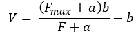
   With F_max being the maximum 100-Hz isometric torque at 70°, F and V representing the isotonic load clamp’s torque and the angular velocity, respectively, and a and b representing Hill’s thermodynamic constants with the units of torque (N•m) and velocity (°/s), respectively.
   NOTE: After the code has picked through each set of force and velocity data, it will produce a new Excel file containing, for each fitted curve, the following data: maximum shortening velocity (V_max), F_max, the a and b coefficients, the torque-velocity curve’s curvature (a / F_max), peak power, the torque value that corresponds to peak power, the angular velocity value that corresponds to peak power, and the R² value representing how well the collected data fits the equation (Figure 4).

9. Comparison of the isotonic and isokinetic torque-velocity-power profiles

1. To eliminate risk of biases related to testing order, 1) alternate between running the isotonic tests first and running the isokinetic tests first; and 2) randomize the contraction order within each set of isotonic (load clamps of 10, 20, 30, 40, 50, 60, 70, and 80% maximum torque) and isokinetic (angular velocities of 50, 100, 200, 300, 400, 600, 800, and 1000°/s) contractions. Select the range of isokinetic angular velocities in accordance with previous studies on the in-vivo rat plantar flexors²³.
2. Use a two-way repeated measures ANOVA to assess similarities and differences between the torque-velocity-power curves produced from the three methods employed here (isotonic, isokinetic with average torque during shortening, and isokinetic with peak torque during shortening) for the following variables: V_max, the a and b coefficients, curvature, peak power, torque at peak power, angular velocity at peak power, and R². Apply a Bonferroni correction to all pairwise comparisons. Set the alpha level to α = 0.05.

Results

Figure 5A shows the torque-velocity relationships generated from the raw data points, and Figure 5B uses the average F_max and a and b coefficients to plot these data fitted to Hill's equation¹ along with the torque-power curves, in which torque and velocity were multiplied together to calculate power. All methods (isotonic, isokinetic using average torque, isokinetic using peak torque) showcase the expected shape of the torque-velocity relationship, with angular shortening velocity decreasing hyperbolically with increasing torque, and vice versa, and with peak power produced at submaximal levels of both torque and velocity.

Figure 6 shows the data obtained from curve-fitting the torque and angular velocity data. The curve yielded from the isotonic tests predicts a greater V_max than both isokinetic curves (P = 0.002 compared to both; Figure 6A). The isotonic curve also yielded a greater peak power than the isokinetic curve using average torque (P = 0.006), but this discrepancy was overcome by instead using peak torque from the isokinetic tests, yielding a peak power that did not differ from that of the isotonic curve (P = 1.00) (Figure 6B). This increase in peak power using peak torque in the isokinetic curve was accomplished mathematically by reducing the curvature of the torque-velocity curve compared to using average torque (P < 0.001) (Figure 6G), despite maintaining the same V_max (P = 1.00) (Figure 6A). This reduction in curvature due to using peak torque from the isokinetic tests also resulted in an overestimation of torque at peak power compared to the isotonic curve (P < 0.001), whereas the isokinetic curve using average torque better matched torque at peak power from the isotonic curve (P = 1.00) (Figure 6C). With that said, the isokinetic curve using average torque underestimated velocity at peak power compared to the isotonic curve (P < 0.001) (Figure 6D). Using peak torque for the isokinetic curve brought velocity at peak power closer to that of the isotonic curve, but with still a slight underestimation (P = 0.043) (Figure 6D). Lastly, while all datasets fitted the Hill equation (all R² > 0.98) strongly, the isotonic curve was a slightly weaker fit than the other two (P = 0.015-0.029). Collectively, these findings demonstrate how constant-load dynamic contractions, which better resemble real-world movements, yield different results compared to the more commonly used constant-velocity dynamic contractions in assessing the torque-velocity-power relationship.

All individual data are publicly available at: https://doi.org/10.6084/m9.figshare.29099018.v2

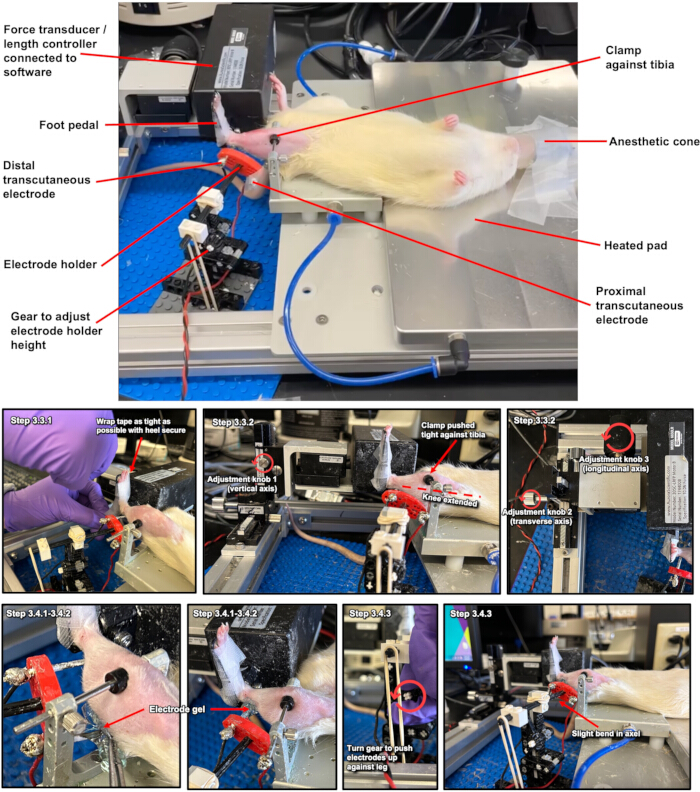
Figure 1: Depiction of how the rat is setup for in vivo testing of plantar flexor mechanical function. The rat is positioned on a heated platform under isoflurane anesthetic. The foot is taped tightly to the foot pedal with the heel secure, and a clamp is pushed into the tibia to fix the lower leg in place. Adjustment knobs 1, 2, and 3 assist with optimal positioning of the leg in a knee-extended position and anatomical alignment with the foot pedal's axis. Conductive gel is spread over the proximal and distal sites of the plantar flexor muscle group. The electrode holder secures the electrodes in place for transcutaneous stimulation. The gear on the custom electrode holding device pushed the electrodes up against the skin overlying the plantar flexor muscles. Please click here to view a larger version of this figure.

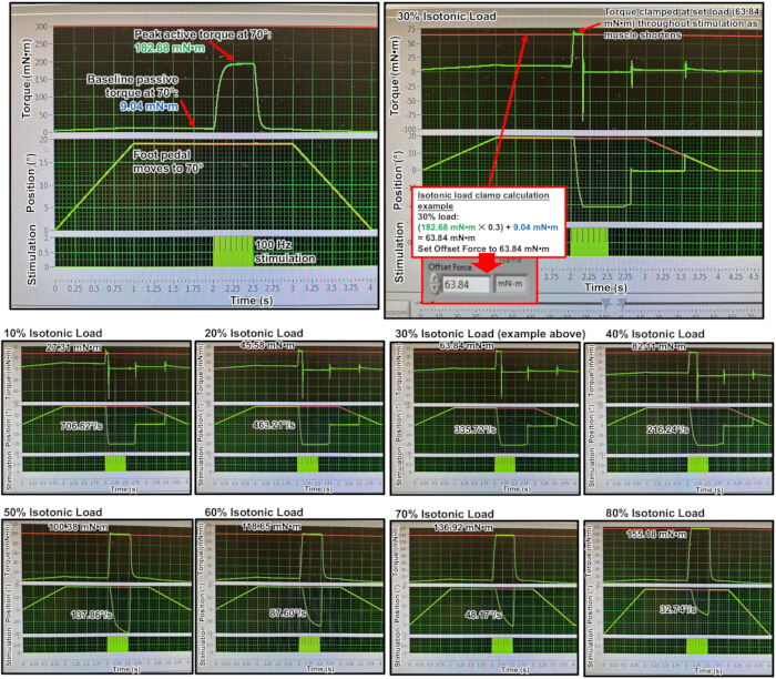
Figure 2: Example raw torque, position, and stimulation traces for a 100 Hz isometric stimulation at a 70° ankle angle, which was then used to determine peak torque in isotonic contractions with loads set at 10% to 80% of peak torque. Included is an example of calculating and setting the isotonic load for a 30% isotonic contraction. Note that in setting the load clamp ("Offset Force"), the calculated load represents a percent of the peak 100 Hz active torque (i.e., total torque minus baseline passive torque), but the baseline passive torque is added back on because the system cannot distinguish between total torque and active torque. Please click here to view a larger version of this figure.

Figure 3: Example raw torque and position traces of isokinetic contractions, from which peak and average torque were measured during shortening. The tests presented are at speeds of 50, 100, 200, 300, 400, 600, 800, and 1000°/s (indicated in the position trace panels). Dashed vertical lines in the "Stimulation" readout indicate the start and end of electrical stimulation (real stimulation is not visible in these photographs of the data readouts). Please click here to view a larger version of this figure.

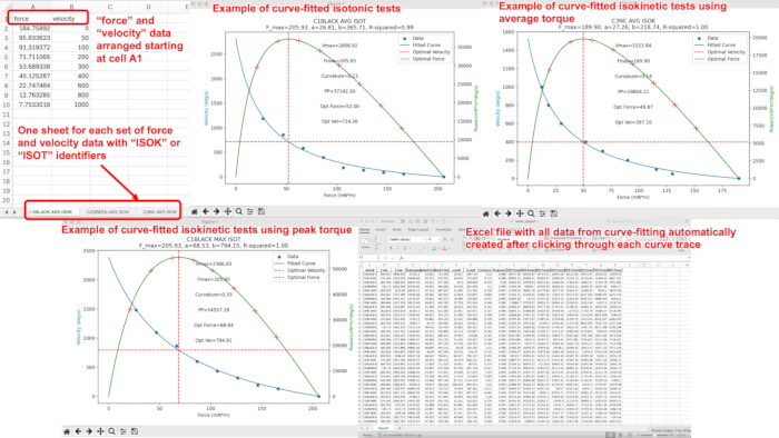
Figure 4: Depiction of the steps required for curve-fitting the torque (labeled as "force" here) and velocity data. After arranging each individual set of torque and velocity data in its own sheet labeled as [Rat name] [ISOK or ISOT] (ISOT = isotonic, ISOK = isokinetic), the code is run. A window will appear prompting an Excel file to be selected. After selecting the file containing all the labeled sheets, each curve will appear one at a time, allowing them to be visually inspected to ensure there are no errors in the data entered. Each curve showcases the maximum shortening velocity (V_max), the maximum torque value (F_max) which would have been input from the measured data, the curve's a and b coefficients, the torque-velocity curve's curvature (a / F_max), peak power, the torque value that corresponds to peak power ("Opt Force"), the angular velocity value that corresponds to peak power ("Opt Vel"), and the R² value representing how well the collected data fits the equation. After clicking through each curve, an Excel file will be automatically generated containing all data produced from curve-fitting for each curve that was just clicked through. Remember to save this file before closing. Please click here to view a larger version of this figure.

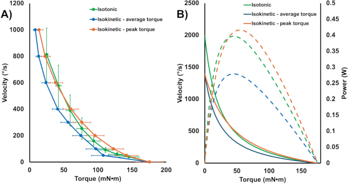
Figure 5: Torque-angular-velocity-power curves. (A) The torque-angular velocity curves constructed from raw data for the isotonic tests (green), the isokinetic tests using average torque during shortening (blue), and the isokinetic tests using peak torque during shortening (orange). (B) The average curves generated from fitting these data to Hill's equation¹ along with the torque-power curves created from multiplying torque and angular velocity together. Data in panel A are presented as the mean ± standard deviation. Please click here to view a larger version of this figure.

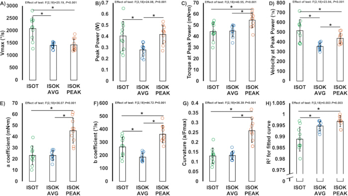
Figure 6: Data obtained from curve-fitting the torque and angular velocity data. Comparison of (A) V_max, (B) peak power, (C) torque at peak power, (D) velocity at peak power, (E) the a coefficient, (F) the b coefficient, (G) curvature, and (H) R² between the curves generated from the isotonic tests (ISOT), isokinetic tests using average torque (ISOK AVG), and isokinetic tests using peak torque (ISOK PEAK). ^*Significant difference (P < 0.05). Data are presented as the mean ± standard deviation. Please click here to view a larger version of this figure.

Supplementary File 1: Electrode holder building instructions and 3D printing files (https://doi.org/10.6084/m9.figshare.28574951.v1)

Supplementary File 2: .dpf protocol files for Aurora Scientific's 3-in-1 system (https://doi.org/10.6084/m9.figshare.29099018.v2)

Supplementary File 3: Python code for curve-fitting torque-angular velocity data (https://github.com/ahinks192/Torque-Velocity-Curve)

Discussion

The present study showcases a novel setup for in vivo testing of rat plantar flexor mechanical function using transcutaneous electrical stimulation. Specifically, the present study demonstrates how to assess the torque-angular velocity-power relationship using isotonic contractions, which better align with the constant-load, velocity-dependent conditions of movements that occur outside the laboratory than isokinetic contractions. Nevertheless, how measurements from an isokinetic torque-angular velocity-power relationship may be optimized to mimic results from isotonic contractions are also presented. Due to the repeatable nature of this experimental setup, these assessments of joint-level dynamic performance have the potential to vastly improve understandings of how age, disease, immobilization, and various exercise interventions impact muscle contractile function in rodent models. Indeed, this setup has previously been used to compare plantar flexor mechanical function between young and old rats, and before and after casting and training interventions^{35,36,37,38,28}.

An important advantage of employing the isotonic protocols over the isokinetic protocols is that the isotonic protocols can be more individualized to a given rat. The isotonic protocols begin with determination of maximum torque production capacity, then the load clamps are normalized to that specific value (i.e., the isotonic curve has variation in both the torque and velocity axes in Figure 5A). With the isokinetic protocols, V_max cannot be determined upfront, thus, it is not possible to normalize the range of submaximal angular velocities to a maximum velocity value and instead use a standardized range of angular velocities (i.e., the isokinetic curve only has variation in the torque axis). This standardized range could become a problem for rats that intrinsically have a slower velocity-production capacity (e.g., with aging^16,40), as the tests would only capture a smaller range of their torque-angular velocity curve, with some of the standardized velocities potentially falling near or beyond V_max. Isotonic contractions, therefore, allow better confidence in capturing a complete representation of the torque-angular velocity curve, and thus power production, at any point in time for any health status. In other words, as recently noted by Thompson¹⁸, isokinetic tests provide no distinction between peak torque and power measurements because velocities are constrained across all participants, whereas isotonic tests decouple torque and power measurements by individualizing the loads to a given participant's maximum torque capability and better capturing the trade-off between torque and velocity.

The ability for better individualization of isotonic contractions may explain why the torque-velocity-power relationship constructed from isotonic contractions yielded a higher V_max than either of the isokinetic methods (Figure 6A). Hence, if a study's primary aim is to assess changes in V_max (e.g., before compared to after a training intervention), isotonic contractions should be used because isokinetic contractions could underestimate this value. However, if a study is instead interested in elucidating changes in peak power, power values yielded from isokinetic contractions can be similar to isotonic contractions by recording peak torque (as opposed to average torque) during isokinetic shortening (Figure 6B).

Measuring torque at peak power and velocity at peak power can also be valuable for assessing whether production of torque or velocity is more relied upon for dynamic performance. For example, if a disease exhibits no change in peak power but an increase in torque at peak power and a decrease in velocity at peak power, this disease then disproportionately affects velocity, and torque production compensates to preserve power output. If attempting to obtain values of torque at peak power and velocity at peak power from isokinetic contractions that are similar to values obtained from isotonic contractions, both isokinetic methods showcased in the present study should be employed. For torque at peak power, recording average torque from isokinetic contractions closely matches that obtained from the isotonic torque-velocity relationship (Figure 6C). Conversely, for velocity at peak power, recording peak torque from isokinetic contractions more closely matches that obtained from the isotonic torque-velocity relationship, however, still with a 15% underestimation (Figure 6D). A recent commentary¹⁸ noted that, if aiming to comprehensively describe a muscle's functional capabilities, it may be desirable to record both isotonic and isokinetic tests regardless, with isotonic tests recommended for assessing peak power and isokinetic tests necessary for assessing peak torque production during muscle shortening.

The experimental setup showcased in the present study also has advantages to improve lab workflow compared to traditional methods (e.g., indwelling electrodes, peripheral nerve cuffs) of assessing in vivo mechanical performance in rodents. The custom electrode holder permits quick adjustment of the height of the electrodes, and adjustment of the distance between the electrodes (via the holes in the red electrode holder piece; Figure 1) to suit any individual rat's leg length. These features also make it easier to match electrode placement/location on the same rat between separate testing sessions, which is especially useful for longitudinal training studies. Indeed, a typical resistance training session (4 sets of 8-10 repetitions) on this setup has been completed at a rate of ~15 min per rat, or 10 rats in ~2.5 h with continuous testing^35,36,37. Additionally, while it is not the focus here, the present research group has developed a smaller electrode holder piece for testing of the mouse plantar flexor in vivo mechanical function as well⁴¹.

Despite the methodological advantages of this setup, there are some limitations to note. Here we used an ankle range of motion of 70° to 110° because that is the limit of the force transducer system we used, and a more extended leg position to optimize torque production as informed by our previous experiments^{35,36,37,38,28}-however, this setup allows for modification of these positions (e.g., bent knee position, different ankle range of motion, different activation settings) to fit a given researcher's experimental needs. It should also be noted that this setup does not fully capture the dynamic, variable-length behavior characteristic of in vivo muscle function during locomotion, as changes in loading can occur during transitions between joint angles that unfortunately cannot be implemented into these controlled single-joint experiments. Lastly, the present protocol used Hill's equation to fit the torque and angular velocity data, which assumes a hyperbolic-shaped curve. While this curve shape is reliable for determining peak power (which occurs at submaximal levels of force and velocity), it may overestimate V_max due to the often-observed double-hyperbolic shape of the force-velocity relationship^2,42. Hence, if a researcher's aim is to primarily assess V_max using the experimental setup presented here, it could be recommended to fit these data to a more complex double-hyperbolic curve as well^2,42.

The isotonic and isokinetic torque-angular velocity-power relationships presented here all had strong (R² > 0.98) fits to Hill's equation (Figure 6H). However, given the limitations noted above for isokinetic torque-angular velocity-power relationships, using isotonic tests is recommended when possible, especially if aiming to assess peak power. If isokinetic tests must instead be used, this article's findings can be used as a guide to understand the limitations and maximize the translatability to constant-load contractions.

Materials

List of materials used in this article

Name	Company	Catalog Number	Comments
1-1/2” steel galvanized smooth finishing nails	The Hillman Group Canada ULC, Pickering, Ontario, Canada	https://shop.hillmangroup.ca/ccrz__ProductDetails?sku=461146&cclcl=en_US	For the custom-made electrode holder (building instructions provided in Supplementary Figure 1)
Apparatus for Rats	Aurora Scientific Inc. (Aurora, Ontario, Canada)	806D
Custom electrode-holding attachment designed in Tinkercad (open source software) and 3D-printed	Autodesk Tinkercad	www.tinkercad.com	For the custom-made electrode holder (building instructions provided in Supplementary Figure 1)
High-Powered, Bi-Phase Stimulator	Aurora Scientific Inc. (Aurora, Ontario, Canada)	701C
LEGO parts	BrickLink.com	See Supplemental Figure S1 for the BrickLink.com codes for all LEGO® parts	For the custom-made electrode holder (building instructions provided in Supplementary Figure 1)
Spectra 360 Electrode Gel	Spectra	https://www.orthocanada.com/en/spectra-electrode-gel?utm_term=&utm_campaign=Canada+EN+-+Search+-+OrthoCanada&utm_source=adwords&utm_medium=ppc&hsa_acc=1971735470&hsa_cam=136169080&hsa_grp=139530010212&hsa_ad=586754644289&hsa_src=g&hsa_tgt=dsa-19959388920&hsa_kw=&hsa_mt=&hsa_net=adwords&hsa_ver=3&gad_source=1&gad_campaignid=136169080&gbraid=0AAAAAD1V26BmzV4eR9tkH_8Truu4W7uu6&gclid=Cj0KCQjwnJfEBhCzARIsAIMtfKLpFSpoPZdXDBtyR8sRgHYCfYuELZFPs4g8U6r8t4_chBuz5KF0pBIaAoQ3EALw_wcB
Systane Nighttime Lubricant Eye Ointment	Systane	https://www.amazon.ca/dp/B004RSQGWC?ref=nb_sb_ss_w_as-reorder_k0_1_12&=&crid=38CVEZ82H7F4&=&sprefix=eye+ointment
Ten female Sprague-Dawley rats	Charles River Laboratories (Senneville, QC, Canada)	Strain code: 001
Transpore Surgical Tape	3M (Milton, Ontario, Canada)	1527
Veet Pure Hair Removal Cream	Veet	https://www.walmart.ca/en/ip/Veet-Pure-Hair-Removal-Cream-Legs-Body-Sensitive-Skin-400-mL/10032637
Water Heater/Circulator	Aurora Scientific Inc. (Aurora, Ontario, Canada)	827A

References

- Hill, A. V., Sec, R. S. The heat of shortening and the dynamic constants of muscle. Proc R Soc Lond B Biol Sci. 126 (843), 136-195 (1938).
- Alcazar, J., Csapo, R., Ara, I., Alegre, L. M. On the shape of the force-velocity relationship in skeletal muscles: the linear, the hyperbolic, and the double-hyperbolic. Front Physiol. 10, 769(2019).
- Araújo, C. G. S., et al. Muscle power versus strength as a predictor of mortality in middle-aged and older men and women. Mayo Clin Proc. 100 (8), 1319-1331 (2025).
- Farris, D. J., Sawicki, G. S. Human medial gastrocnemius force-velocity behavior shifts with locomotion speed and gait. Proc Natl Acad Sci U S A. 109 (3), 977-982 (2012).
- Clemente, C. J., Richards, C. Muscle function and hydrodynamics limit power and speed in swimming frogs. Nat Commun. 4, 2737(2013).
- Yeo, S. H., Monroy, J. A., Lappin, A. K., Nishikawa, K. C., Pai, D. K. Phenomenological models of the dynamics of muscle during isotonic shortening. J Biomech. 46 (14), 2419-2425 (2013).
- Lappin, A. K., Monroy, J. A., Pilarski, J. Q., Zepnewski, E. D., Pierotti, D. J., Nishikawa, K. C. Storage and recovery of elastic potential energy powers ballistic prey capture in toads. J Exp Biol. 209 (13), 2535-2553 (2006).
- Charles, J. P., Kissane, R. W. P., Askew, G. N. The impacts of muscle-specific force-velocity properties on predictions of mouse muscle function during locomotion. Front Bioeng Biotechnol. 12, 1436004(2024).
- Jinha, A., Herzog, W. Muscle power: a simple concept causing much confusion. J Sport Health Sci. 14, 101005(2025).
- Andersen, L. L., et al. Changes in the human muscle force-velocity relationship in response to resistance training and subsequent detraining. J Appl Physiol. 99 (1), 87-94 (2005).
- Hinks, A., et al. Power loss is attenuated following a second bout of high intensity eccentric contractions due to the repeated bout effect’s protection of rate of torque and velocity development. Appl Physiol Nutr Metab. 46 (5), 461-472 (2020).
- Dalton, B. H., Power, G. A., Paturel, J. R., Rice, C. L. Older men are more fatigable than young when matched for maximal power and knee extension angular velocity is unconstrained. Age. 37 (3), 49(2015).
- Power, G. A., Dalton, B. H., Rice, C. L., Vandervoort, A. A. Delayed recovery of velocity-dependent power loss following eccentric actions of the ankle dorsiflexors. J Appl Physiol. 109 (3), 669-676 (2010).
- Dalton, B. H., Allen, M. D., Power, G. A., Vandervoort, A. A., Rice, C. L. The effect of knee joint angle on plantar flexor power in young and old men. Exp Gerontol. 52, 70-76 (2014).
- Power, G. A., Dalton, B. H., Rice, C. L., Vandervoort, A. A. Peak power is reduced following lengthening contractions despite a maintenance of shortening velocity. Appl Physiol Nutr Metab. 38 (12), 1196-1205 (2013).
- McNeil, C. J., Rice, C. L. Fatigability is increased with age during velocity-dependent contractions of the dorsiflexors. J Gerontol A Biol Sci Med Sci. 62 (6), 624-629 (2007).
- Knight, K. L., Ingersoll, C. D., Bartholomew, J. Isotonic contractions might be more effective than isokinetic contractions in developing muscle strength. J Sport Rehabil. 10 (2), 124-131 (2001).
- Thompson, B. J. It’s time to re-evaluate the reporting of common measures from isokinetic dynamometers: isokinetic for torque, isotonic for power. Front Sports Act Living. 7, 1472712(2025).
- Leeuwenburgh, C., Gurley, C. M., Strotman, B. A., Dupont-Versteegden, E. E. Age-related differences in apoptosis with disuse atrophy in soleus muscle. Am J Physiol Regul Integr Comp Physiol. 288 (5), R1288-R1296 (2005).
- Padilla, C. J., et al. Profiling age-related muscle weakness and wasting: neuromuscular junction transmission as a driver of age-related physical decline. Geroscience. 43 (3), 1265-1281 (2021).
- Fuqua, J. D., et al. Impaired proteostatic mechanisms other than decreased protein synthesis limit old skeletal muscle recovery after disuse atrophy. J Cachexia Sarcopenia Muscle. 14 (5), 2076-2089 (2023).
- Ochi, E., Nakazato, K., Ishii, N. Effects of eccentric exercise on joint stiffness and muscle connectin (titin) isoform in the rat hindlimb. J Physiol Sci. 57 (1), 1-6 (2007).
- Warren, G. L., Stallone, J. L., Allen, M. R., Bloomfield, S. A. Functional recovery of the plantarflexor muscle group after hindlimb unloading in the rat. Eur J Appl Physiol. 93 (1-2), 130-138 (2004).
- Herzog, W., Leonard, T. R. Force enhancement following stretching of skeletal muscle: a new mechanism. J Exp Biol. 205 (Pt 9), 1275-1283 (2002).
- Lewis, M. T., Kasper, J. D., Bazil, J. N., Frisbee, J. C., Wiseman, R. W. Skeletal muscle energetics are compromised only during high-intensity contractions in the Goto-Kakizaki rat model of type 2 diabetes. Am J Physiol Regul Integr Comp Physiol. 317 (2), R356-R368 (2019).
- Hill, C., James, R., Cox, V., Tallis, J. Does dietary-induced obesity in old age impair the contractile performance of isolated mouse soleus, extensor digitorum longus and diaphragm skeletal muscles. Nutrients. 11 (3), 505(2019).
- Yuan, L., et al. The atypical β-blocker S-oxprenolol reduces cachexia and improves survival in a rat cancer cachexia model. J Cachexia Sarcopenia Muscle. 14 (1), 653-660 (2023).
- Hinks, A., Power, G. A. Age-related differences in the loss and recovery of serial sarcomere number following disuse atrophy in rats. Skeletal Muscle. 14 (1), 18(2024).
- Hulst, J. B., Minamoto, V. B., Lim, M. B., Bremner, S. N., Ward, S. R., Lieber, R. L. Systematic test of neurotoxin dose and volume on muscle function in a rat model. Muscle Nerve. 49 (5), 709-715 (2014).
- Wang, X., et al. Human neural stem cells transplanted during the sequelae phase alleviate motor deficits in a rat model of cerebral palsy. Cytotherapy. 26 (12), 1491-1504 (2024).
- Baltgalvis, K. A., Call, J. A., Cochrane, G. D., Laker, R. C., Yan, Z., Lowe, D. A. Exercise training improves plantar flexor muscle function in mdx mice. Med Sci Sports Exerc. 44 (9), 1671-1679 (2012).
- Sam, M., Shah, S., Fridén, J., Milner, D. J., Capetanaki, Y., Lieber, R. L. Desmin knockout muscles generate lower stress and are less vulnerable to injury compared with wild-type muscles. Am J Physiol Cell Physiol. 279 (4), C1116-C1122 (2000).
- Mintz, E. L., Passipieri, J. A., Lovell, D. Y., Christ, G. J. Applications of in vivo functional testing of the rat tibialis anterior for evaluating tissue engineered skeletal muscle repair. J Vis Exp. (116), e54487(2016).
- Song, H., Nakazato, K., Nakajima, H. Effect of increased excursion of the ankle on the severity of acute eccentric contraction-induced strain injury in the gastrocnemius: an in vivo rat study. Am J Sports Med. 32 (5), 1263-1269 (2004).
- Hinks, A., Patterson, M. A., Njai, B. S., Power, G. A. Age-related blunting of serial sarcomerogenesis and mechanical adaptations following 4 weeks of maximal eccentric resistance training. J Appl Physiol. 136 (5), 1209-1225 (2024).
- Hinks, A. A., Vlemmix, E., Power, G. A. Submaximal eccentric resistance training increases serial sarcomere number and improves dynamic muscle performance in old rats. Physiol Rep. 12 (19), e70036(2024).
- Hinks, A., Vlemmix, E., Power, G. A. Submaximal eccentric training during immobilization does not prevent serial sarcomere loss or impairments in mechanical function in old or young rats. J Gerontol A Biol Sci Med Sci. 80 (7), glaf082(2025).
- Vlemmix, E., Hinks, A., Power, G. A. Serial sarcomerogenesis does not contribute to the initial repeated bout effect in skeletal muscle. J Biomech. 187, 112767(2025).
- Oh, S. S., Narver, H. L. Mouse and rat anesthesia and analgesia. Curr Protoc. 4 (2), e995(2024).
- Paris, M. T., McNeil, C. J., Power, G. A., Rice, C. L., Dalton, B. H. Age-related performance fatigability: a comprehensive review of dynamic tasks. J Appl Physiol. 133 (4), 850-866 (2022).
- Hinks, A., et al. Time course changes in in vivo muscle mechanical function and Ca2+ regulation of force following experimentally induced gradual ovarian failure in mice. Exp Physiol. 109 (5), 711-728 (2024).
- Edman, K. A. Double-hyperbolic force-velocity relation in frog muscle fibres. J Physiol. 404 (1), 301-321 (1988).
Reprints and Permissions