This article introduces a protocol for using DeepSpaceDB, a dynamic, interactive database for spatial transcriptomics, offering analysis workflows and examples to explore tissue organization and disease-related gene expression.
Method Article
Mining Spatial Transcriptomics Datasets using DeepSpaceDB
In This Article
Summary
Abstract
Spatial transcriptomics is a rapidly evolving technology that enables the capture of gene expression patterns in tissue samples while preserving positional information. It has wide-ranging applications in biological research and bioinformatics, allowing researchers to investigate and track spatial variations in gene expression across different tissues, conditions, and diseases. With spatial transcriptomics data analysis gaining traction, the number of publicly available datasets is rising. However, spatial transcriptomics remains a highly specialized experimental technique, with significant technical and financial constraints. To facilitate access to spatial data, we have recently developed DeepSpaceDB, a comprehensive and dynamic database for spatial transcriptomics data exploration. This article presents detailed workflows outlining the components of the database and its navigation with the help of a few examples. First, the analysis of a mouse brain sample is demonstrated, exploring quality indicators, spatially variable genes and pathways, and gene expression variations between the hippocampus and hypothalamus. Next, the identification and annotation of differentially expressed genes associated with immune activity is further explored by comparing metastatic regions of colorectal origin with distant areas of healthy tissue in murine livers. DeepSpaceDB, with its advanced tools and interactive features, serves as a valuable resource for spatial transcriptomics research, enabling deeper exploration of tissue organization and disease biology.
Introduction
Spatial transcriptomics is a new technology that enables researchers to analyze gene expression while retaining spatial information inside a tissue section, thus enabling the study of tissue architecture, cellular heterogeneity, and microenvironmental influences at unprecedented resolution1,2. However, despite the potential of this technology, access and analysis remain limited, spatial transcriptomics is cost-prohibitive for many laboratories, and the data analysis requires advanced bioinformatics skills.
Developing public databases is one way to broaden access to this emerging experimental modality. Several spatial transcriptomics databases have been created. The first was SpatialDB, but it contains only a limited number of samples and has not been updated3. The SODB, SOAR, and STOmicsDB databases include large numbers of samples from many different platforms and serve a great role as data repositories4,5,6. However, analysis tools are limited and lack interactivity. To address this issue, we have recently developed DeepSpaceDB, a curated, user-friendly database of publicly available spatial transcriptomics datasets designed to lower technical barriers and expand accessibility7. This article illustrates several tools in this database, including searching the database, inspecting sample quality, visualization tools, and the comparison of interactively selected regions within tissue slices. It presents detailed protocols using two representative examples: the analysis of a mouse brain sample and a murine liver with colorectal metastases to demonstrate these tools in practical contexts. Through these tools, DeepSpaceDB empowers a broader range of researchers to leverage spatial transcriptomics without needing their own data or in-house bioinformatics capacity. A comprehensive description of the data collection, quality control, processing workflow, as well as the data and features included in DeepSpaceDB, is provided in detail by Honcharuk et al7.
Protocol
1. Example 1: Analysis of a mouse brain sample
NOTE: In this section, the analysis of a mouse brain sample is illustrated, navigating through the different features and plots available in DeepSpaceDB (a link to the database is available in the Table of Materials).
- Sample selection
- Click on the Database tab and use the filter to select the organism mouse, the organ brain, and the source zenodo. Move through the resulting samples, and select sample DSID001557. Alternatively, use the search box to search the database for the term "DSID001557" and select this sample.
- Click on the sample and confirm the description as 2 × 10⁶ cells in 100 µL saline-NK cell (i.v. injection once a week for a total of 5 times).
- Quality analysis
- Click on the Quality tab to evaluate the quality of the selected sample. From the quality measures drop-down menu, select different options like Detected Genes (Figure 1A), Read Count (Figure 1B), and Mito (Figure 1C), to visualize the respective parameters in each spot across the sample slice.
- Image annotation
- Navigate to the Image annotation tab for identifying the different regions of the sample slice.
- Move the mouse cursor over the sample slice. Annotations predicted by a large language model (LLM) are displayed for parts of the sample image in a grid-based manner, with information about the anatomy and associated condition8.
- Cluster analysis
- For a deeper understanding of the cell type clusters in the sample slice, navigate to the Clusters tab. A 2D embedding of the clusters will be displayed, along with a representation of color-coded clusters across the spots on the sample slice (Figure 1E).
- Spatially variable genes and pathways
- Navigate to the Genes tab and take note of the spatially variable genes (SVG; genes whose expression levels differ across tissue locations) in the sample9,10. These SVGs are predicted using the singleCellHaystack function, which adopts the Kullback-Leibler Divergence measure (D_KL in the table) to evaluate how distinct the expression pattern of each gene is from what would be expected at random (Figure 2). Genes with a low p-value (large negative log.p.adj in the table) are listed as the SVGs.
NOTE: Gene expression data was normalized using the default parameters used in the Seurat R (version 5) package11. In practice, the reads for each gene at each spot were divided by the total count of reads in that spot, and multiplied by the scale factor 10,000. Next, the natural logarithm was calculated after addition of 1, to avoid problems with log(0). The plot shown in the Genes tab shows this normalized data. - Click on some of the top genes in the list. This generates a spatial plot for the genes across the tissue slice, with spots color-coded for the expression level (Figure 2). Top-scoring genes have clearly distinct spatial patterns of expression.
- Navigate further to the Pathways tab to inspect the activity of sets of genes (e.g., genes associated with a common biological pathway) rather than individual genes. Spatially variable pathways are listed in a similar way to the SVGs discussed above (Figure 3). Pathway activities are estimated based on the expression levels of the genes associated with them7,11.
NOTE: Pathway activities were estimated using the Seurat R package function addModuleScore11. In brief, this function takes as input a set of genes (e.g., a set of genes involved in a common pathway) and returns their average expression levels, after several processing steps. In practice, positive values imply a higher than average activity, and negative values a lower than average activity. The plot shown in the Pathways tab shows this module score data. - Click on some of the top pathways in the list. This generates a spatial plot for the pathways across the tissue slice, with spots color-coded for the activity level. Several pathways have distinct spatial patterns of activity (Figure 3).
- Navigate to the Genes tab and take note of the spatially variable genes (SVG; genes whose expression levels differ across tissue locations) in the sample9,10. These SVGs are predicted using the singleCellHaystack function, which adopts the Kullback-Leibler Divergence measure (D_KL in the table) to evaluate how distinct the expression pattern of each gene is from what would be expected at random (Figure 2). Genes with a low p-value (large negative log.p.adj in the table) are listed as the SVGs.
- Intra-sample gene expression comparison
- Navigate to the Tissue Explorer tab and select Manual Selection (if it has not yet been selected). Next, use the mouse cursor to select the spots in the hippocampal region of the mouse brain slice, on the left side. Click on set 1, and select add to set. This will highlight all the selected spots on the slice on the right side (Figure 4A).
- Now click on set 2, and use the mouse cursor to select the spots in the hypothalamic region of the mouse brain slice. Click on add to set, which will highlight all the selected spots on the slice on the right side (Figure 4A).
- After completing the spot selection process, click on the Compare gene expression button. This will generate a table with the average gene expression values of the selected spots between both regions, along with a scatterplot representation. Move the cursor over individual spots to confirm the gene names and the average expression of genes in both regions.
- Based on the gene expression comparison results, identify differentially expressed genes and re-navigate to the Genes tab to visualize their expression across the sample slice (Figure 4B,C).
NOTE: Through the steps detailed above, DeepSpaceDB can be used to investigate the features of a mouse brain spatial transcriptomics sample.
2. Example 2: Identification and annotation of differentially expressed genes associated with immune activity in metastatic regions of colorectal origin in mouse livers
NOTE: An intra-sample comparison is explored in the current section. This is illustrated through the identification and annotation of differentially expressed genes between metastatic regions of colorectal origin, and distant regions of healthy tissue within a liver section, based on two different samples. The spatial expression of specific dysregulated genes relevant to immune activity is further visualized in the tissue sections.
- Database navigation and sample selection
- Click on the Database tab and use the filter to select the organism mouse, the organ liver, and the condition cancer. From the resulting samples, select sample DSID001005. Click on the sample and confirm the description stating that the sample is from a mouse liver containing metastasis of colorectal cancer origin.
- Navigate to the Tissue Explorer tab and select Manual Selection. Next, using the mouse cursor, select the spots in the tumor region (colorectal metastases) of the liver sample DSID001005, identified based on the positive expression of the Epcam marker (Figure 5A). Click on set 1, and select add to set. This highlights all the selected spots on the slice on the right side (Figure 5C).
- Now click on set 2, and use the mouse cursor to select the spots in the distant non-tumor region of the liver sample. Click on add to set, which will highlight all the selected spots on the slice on the right side (Figure 5C).
- Comparison of gene expression between selected spots
- After completing the spot selection process, click on the Compare gene expression button. This generates a table with the average gene expression values of the selected spots between both regions, along with a scatterplot representation. Move the mouse cursor over individual spots and inspect the gene names and the average expression of genes in both regions.
- To conduct a deeper analysis with the gene expression data, select the Download CSV option. This generates a Comma-Separated Values (CSV) file of the gene expression data for the two regions of the sample.
- Repeat steps 2.1.1-2.1.3 and 2.2.1-2.2.2 for sample "DSID001007". Confirm its description as another slice from a mouse liver containing metastases of colorectal cancer origin.
- Data analysis with R programming
- Confirm that the steps above resulted in 2 CSV files, one from sample DSID001005 and one from sample DSID001007. Both files contain 2 columns representing the average gene expression in the 2 selections (tumor tissue and non-tumor tissue) that were made in each sample.
- Read the CSV files into R and merge them for further downstream analysis with two replicates per condition (i.e., tumor region with colorectal cancer metastases, and distant healthy tissue in the liver). Refer to the R script and data files in the Supplementary materials.
- Use the limma package (version 3.62.2) in R (version 4.4.2)12 to conduct differential expression analysis for the data, categorizing the colorectal metastases regions of both samples as cancer, and the distant, healthy regions of both samples as control. Obtain the upregulated genes with a filter of logFC > 0.5 and adjusted p-value < 0.05. Similarly, obtain the downregulated genes with a filter of logFC < -0.5 and adjusted p-value < 0.05.
NOTE: These sets of genes are used to identify biological pathways that are affected by the tumor in the next step (Figure 6A,B). - Use the clusterProfiler package (version 4.14.6) in R13 to conduct the analysis of pathways of the Kyoto Encyclopedia of Genes and Genomes (KEGG)14 for the downregulated and upregulated genes. Based on a stringent filter of q-value < 0.05, identify the significant pathways associated with the downregulated and upregulated genes. Focus on genes associated with immunological pathways, immune activities, or relevant signatures (Figure 6B).
- Gene-specific data mining
- Next, search for gene names in the Spatially Variable Genes section to confirm the spatial expression of the target genes. Click on a gene name to generate a spatial plot for the gene across the tissue slice, with spots color-coded for the expression level (Figure 7).
- Identify specific genes with spatial patterns of expression at the site of colorectal metastases, as against the distant, healthy liver tissue. The functional relevance of the genes, or their expression in other organs or conditions can be further explored in the database.
- Select the Search tab, and choose the species as mouse. Click on the search by gene option, and type in a gene name. An overview of the organ and condition distribution of the genes will be displayed and can be further analyzed.
NOTE: Through the steps detailed above, DeepSpaceDB can be used to investigate gene expression patterns between metastatic and non-metastatic regions in mouse liver spatial transcriptomics samples.
Results
Example 1 demonstrated the analysis of a mouse brain sample, validating parameters like read count, spatially variable genes and pathways, and gene expression variations between the hippocampus and cortex. First, the quality of the mouse brain sample DSID001557 was assessed against several quality measures: "Detected Genes" (Figure 1A), "Read Count" (Figure 1B), and "Mito" (the percentage of mitochondrial reads; Figure 1C). This clearly highlighted a region with lower quality on the left side of the brain sample, based on the low number of detected genes and the low read count. To understand the relative quality of the sample against all other samples, the Relative quality of sample tab in the database was clicked, which displayed a graph of the Count versus No. of genes detected per spot (Mean). For the sample being analyzed, there were between 3500-4000 genes detected per spot (Figure 1D). The anatomical features of the sample were further analyzed using the Image annotation tab. As a general note, these annotations have been generated by cutting tissue images into smaller parts and asking an LLM to describe the observable features8. They are rough indications to assist the interpretation of the sample and need to be interpreted with care. For a subset of samples (especially human breast cancer samples), annotations by a human specialist are also available. However, considering the lower quality of Visium H&E images compared to images used for routine diagnosis, the provided annotations are for research purposes only. For sample DSID001557, move the cursor over the slice displayed annotations of the different regions of the mouse brain, such as the hippocampal region, cortical layers, dense cellular layers with gliosis, etc. From understanding the basic anatomical features of the sample slice, detailed features like cell type clusters and spatially variable genes and pathways were further explored. The mouse brain sample had 15 clusters in total, which were represented with color coding across the sample slice (Figure 1E). Some of the top spatially variable genes associated with the sample are Nrgn, Slc17a7, Ly6h, and Ddn (Figure 2). Nrgn exhibited high expression in the hippocampal region, in accordance with the literary evidence that indicates the role of the Nrgn-encoded protein (neurogranin) in mediating synaptic plasticity and spatial learning15. Slc17a7, a gene coding for a vesicular glutamate transporter crucial for neurotransmission in glutaminergic neurons16, and Ddn, a gene coding for a protein that modulates the structure of the post-synaptic cytoskeleton17, were also highly expressed in the hippocampal region. In contrast, the expression of gene Ly6h was localized in the cortical region, in accordance with the literature that indicates the restrictive synaptic role of Ly6h in the membranes of cortical cells18. In a similar way, the activity of pathways was visualized across the sample slice (Figure 3). The spatially variable pathways were observed to be activated in concordance with the functional roles of the spatially variable genes, with regulation of synaptic plasticity and neurotransmitter activity in the hippocampal region, and neuropeptide signaling in the cortical region.
Finally, to identify differentially expressed genes between the hippocampal region and the hypothalamus of the mouse brain sample, the Tissue Explorer tab was utilized. Spots associated with the regions of interest were selected with guidance from the image annotation (Figure 4A). From the scatterplot generated, some of the differentially expressed genes identified were among the top spatially variable genes (Nrgn, Slc17a7, Ddn), in addition to a few others, such as Pmch and Ttr. The expression of these genes was visualized in the sample slice. Pmch was specifically overexpressed in the lateral hypothalamic region (Figure 4B; compare with the green selected area in Figure 4A). This gene encodes the precursor of the melanin concentrating hormone, and is involved in the maintenance of energy homeostasis19. In contrast, the gene Ttr was specifically expressed in the hippocampal region (Figure 4C; compare with the red selected area in Figure 4A), in accordance with its functional role in learning and spatial memory20. By conducting intra-sample comparisons between different mouse brain regions using this database, we were able to highlight region-specific functional features based on spatial gene expression and pathway activity.
In example 2, the database was utilized for the identification of immune signatures associated with colorectal metastases in the liver. Intra-sample comparison was conducted between the tumor region with colorectal metastases and the distant, healthy liver tissue, through appropriate spot selection for the two samples: DSID001005 (Figure 5A-C) and DSID001007 (Figure 5D-F). The data were re-analyzed with two replicates per condition using R. Differential expression analysis conducted between the tumor region with colorectal metastasis and the healthy liver tissue revealed the downregulation of 138 genes and the upregulation of 115 genes, based on the selected parameters (Figure 6A,B). KEGG pathway analysis demonstrated the enrichment of the downregulated genes' pathways, like drug metabolism and chemical carcinogenesis (Figure 6C), while the upregulated genes exhibited signatures corresponding to leukocyte trans-endothelial migration, focal adhesion, and cell cycle, among others (Figure 6D). Focusing on the relevance of leukocyte trans-endothelial migration for immune activity, top genes detected in the category were identified, and their spatial expression was observed in DeepSpaceDB. Interestingly, genes Cldn7, Cldn4, and Actg1 detected under the category of leukocyte trans-endothelial migration, exhibited upregulation at the tumor region (Epcam+ site) of the samples, and not in the distant region with healthy liver tissue (Figure 7). This provided insights into the nature of the immune activity driven at the tumor site of the liver, with the active recruitment of leukocytes. In summary, intra-sample analysis using DeepSpaceDB enables the extraction of diverse biological insights. By comparing spatial transcriptomic data through interactive tools and re-analysis workflows, researchers can generate and validate hypotheses regarding tissue-specific gene expression and functional heterogeneity.
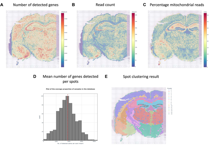
Figure 1: Quality measures of the sample. (A) Number of detected genes, (B) read count, and (C) percentage mitochondrial reads per spot. (D) The average number of detected genes per spot in this sample, compared to the distribution of all other samples in the database. (E) Spot clusters across the tissue slice. Please click here to view a larger version of this figure.

Figure 2: Expression of top spatially variable genes. (A) Nrgn, (B) Slc17a7, (C) Ly6h, and (D) Ddn. Please click here to view a larger version of this figure.
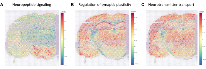
Figure 3: Activity of top spatially variable pathways. (A) Neuropeptide signaling, (B) Regulation of synaptic plasticity, (C) Neurotransmitter transport. Please click here to view a larger version of this figure.
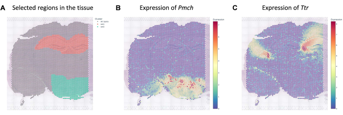
Figure 4: Comparison of gene expression patterns between two selected regions of the mouse brain. (A) Spot selection in hypothalamic and hippocampal regions for intra-sample comparisons. Selected region 1 is shown in red, and region 2 in green. Spatial expression patterns of differentially expressed genes (B) Pmch and (C) Ttr between hypothalamic and hippocampal regions. Please click here to view a larger version of this figure.
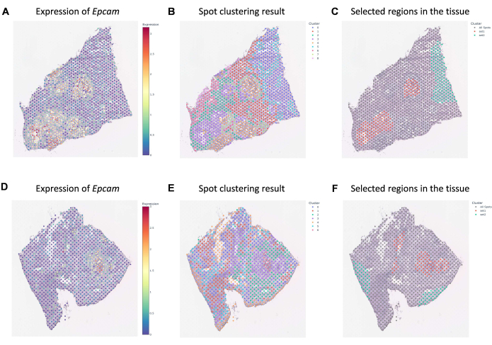
Figure 5: Properties of two metastatic mouse liver samples. For sample DSID001005: (A) Epcam marker expression, (B) spot clusters, and (C) selected regions in cancerous and distant regions for intra-sample comparisons. For sample DSID001007: (D) Epcam marker expression, (E) spot clusters, and (F) selected regions in cancerous and distant regions for intra-sample comparisons. For both samples, tumor spots are in the regions shown in red, and non-tumor spots are in the regions shown in green. Please click here to view a larger version of this figure.
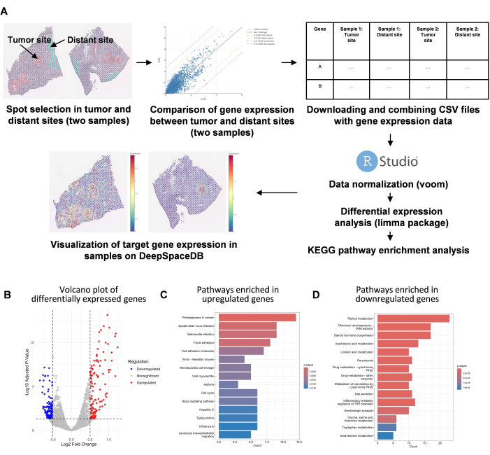
Figure 6: Re-analysis results. (A) Schematic summary of the workflow used in the re-analysis. (B) Volcano plot representing the differentially expressed genes between cancerous and distant regions. KEGG pathway enrichment of (C) upregulated genes and (D) downregulated genes. Please click here to view a larger version of this figure.
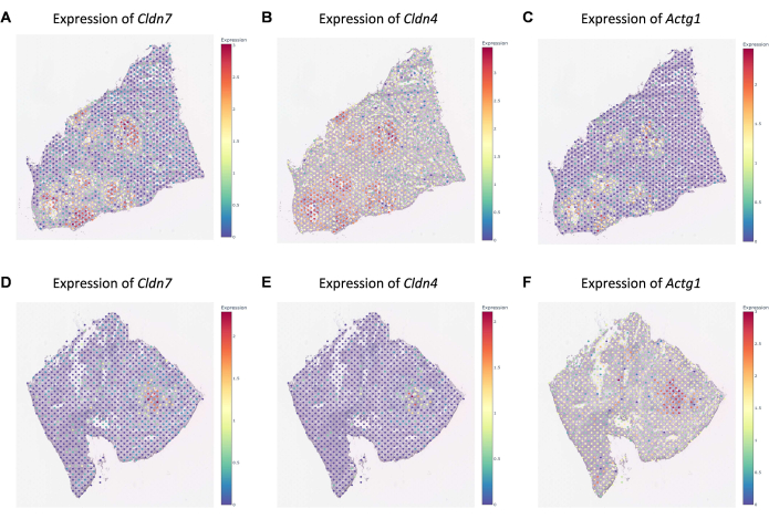
Figure 7: Spatial expression of genes. (A) Cldn7, (B) Cldn4, and (C) Actg1 in tissue slice DSID001005. Spatial expression of genes. (D) Cldn7, (E) Cldn4, and (F) Actg1 in tissue slice DSID001007. Please click here to view a larger version of this figure.
Supplementary files 1-4: Data files and R script for liver metastasis example. Please click here to download this File.
Discussion
Here, we introduced two comprehensive protocols outlining the navigation, retrieval, and analysis of spatial transcriptomics data in DeepSpaceDB. While most spatial omics databases focus on the collection of data from a large number of samples, generated using various platforms3,4,5,6, DeepSpaceDB focuses on the development of interactive tools that allow users to deeply and efficiently explore spatial transcriptomic features. To enable this level of functionality, the current release focuses exclusively on the Visium platform. With the emergence of high-resolution platforms, we plan to expand DeepSpaceDB accordingly, developing new strategies for the processing and integration of such data in a user-friendly manner.
DeepSpaceDB enables users to assess sample quality metrics (e.g., gene counts, read depth) and compare them across datasets. The database includes multi-layered annotations: unsupervised clustering across the full database with assigned labels, LLM-based detection of structural and pathological features from histological images, and expert histology annotations for a growing subset of samples. Moreover, users can interactively select regions of interest within or across samples to compare gene expression, enabling studies of spatial contrasts between regions like tumor versus stroma or diseased versus healthy regions. Such features are generally lacking in other databases3,4,5,6. Other features, such as spatially variable genes and pathways, cell type predictions, and clustering results, are also available. Taken together, this database significantly lowers the barriers to exploring spatial transcriptomics data. Samples from a wide range of tissues and conditions are freely accessible, and users can navigate them through simple point-and-click interactions; no advanced bioinformatics expertise required. That said, some prior knowledge of marker genes and tissue architecture is likely necessary for the accurate interpretation of expression patterns and for selecting regions of interest in the Tissue Explorer tool.
Although not introduced here, users can also upload their own samples and apply many of the same tools to analyze them. The database also supports inter-sample comparisons between 2 different tissue slices, allowing, for example, comparisons between diseased tissues and healthy control tissues. Finally, raw and processed data, along with all derived analysis outputs, are available for download, supporting downstream workflows and custom analyses. For several of these tools, short tutorial videos are available on the tutorial page of the database.
There are still aspects of the database that require improvement. One is the accurate prediction of cell types and cell type compositions at each location within the tissue slices. In the current version of DeepSpaceDB (version 1.0), we predicted the cell type composition of each Visium spot using a method called robust cell type decomposition (RCTD)21. RCTD performed relatively well in a recent benchmark study22. Predictions made by RCTD could also be experimentally validated in our recent study of the livers of cancer-bearing mice23. However, a comprehensive evaluation of the accuracy of cell type predictions has not been conducted. A related issue is that RCTD and other cell type prediction methods require a reference dataset with annotated cell types. In general, cell types (or cell type compositions) at each spatial location are predicted through the comparison with gene expression patterns in this reference dataset. However, selecting a suitable reference for each Visium sample is not always straightforward. References might lack key cell types, or, conversely, might include cell types that are not present in the tissue slice24. Moreover, within one cell type, cells can be in drastically different states, such as inactive versus activated immune cells25. The cell states present in reference datasets don't necessarily match those of spatial samples, which are often obtained from disease models of patients. Both issues are likely to result in inaccurate predictions. We hope to address this issue in the future.
As the field of spatial transcriptomics continues to evolve rapidly, a growing number of computational tools are being developed to analyze diverse aspects of spatial data, including cell-cell interactions, spatial domains, and prediction of spatially variable genes (see, for example 26,27,28). While this proliferation reflects the field's dynamism, it also presents a challenge for curating and integrating tools into this database. To ensure that the most robust and broadly applicable methods are included, there is a pressing need for systematic benchmark studies that evaluate tool performance across datasets and analysis tasks22,29,30. Such efforts will be essential to guide informed selection and prioritization of tools for inclusion in the database.
While other spatial transcriptomics databases attempt to collect large numbers of samples of many different platforms, in DeepSpaceDB we have decided to use a different strategy: focus on a few popular platforms and implement interactive and intuitive tools that allow the user to easily explore the data in more detail. Although our database contains only Visium samples in the current version 1.0, we plan to also include samples from other platforms in a future update.
Disclosures
The authors have nothing to disclose.
Acknowledgements
The authors would like to thank Y. Harada for secretarial assistance. This work was supported by JST NBDC (Grant Number JPMJND2303, A.V.) and AMED (Grant Number JP24gm2010003, A.V.) This work was also supported by JSPS KAKENHI (20H03451, 24K02236, and 24KK0147; S.K.), JST FOREST (JPMJFR2062; S.K), JST Moonshot (JPMJMS2011-61; S.K). The funders had no role in study design, data collection and analysis, decision to publish, or preparation of the manuscript.
Materials
| Name | Company | Catalog Number | Comments |
|---|---|---|---|
| clusterProfiler | R package - version 4.14.6 | ||
| DeepSpaceDB | version > 1.0 | A link to the database: www.deepspacedb.com | |
| limma | R package - version 3.62.2 | ||
| R | version 4.4.2 | ||
| RStudio | Posit | version 2024.12 |
References
- Tian, L., Chen, F., Macosko, E. Z. The expanding vistas of spatial transcriptomics. Nat Biotechnol. 41 (6), 773-782 (2023).
- Moses, L., Pachter, L. Museum of spatial transcriptomics. Nat Methods. 19 (5), 534-546 (2022).
- Fan, Z., Chen, R., Chen, X. SpatialDB: A database for spatially resolved transcriptomes. Nucleic Acids Res. 48 (D1), D233-D237 (2020).
- Yuan, Z., et al. SODB facilitates comprehensive exploration of spatial omics data. Nat Methods. 20 (3), 387-399 (2023).
- Xu, Z., et al. STOmicsDB: A comprehensive database for spatial transcriptomics data sharing, analysis and visualization. Nucleic Acids Res. 52 (D1), 1053-1061 (2024).
- Li, Y., et al. SOAR elucidates biological insights and empowers drug discovery through spatial transcriptomics. Sci Adv. 11 (24), 7450(2025).
- Honcharuk, V., et al. DeepSpaceDB: A spatial transcriptomics atlas for interactive in-depth analysis of tissues and tissue microenvironments. bioRxiv. , (2025).
- GPT-4 technical report. arXiv. , OpenAI. http://arxiv.org/abs/2303.08774 (2023).
- Vandenbon, A., Diez, D. A clustering-independent method for finding differentially expressed genes in single-cell transcriptome data. Nat Commun. 11 (1), 1-10 (2020).
- Vandenbon, A., Diez, D. A universal tool for predicting differentially active features in single-cell and spatial genomics data. Sci Rep. 13 (1), 1-14 (2023).
- Hao, Y., et al. Dictionary learning for integrative, multimodal, and scalable single-cell analysis. Nat Biotechnol. 42 (2), 293-304 (2024).
- Ritchie, M. E., et al. Limma powers differential expression analyses for RNA-sequencing and microarray studies. Nucleic Acids Res. 43 (7), e47(2015).
- Yu, G., Wang, L. G., Han, Y., He, Q. Y. ClusterProfiler: An R package for comparing biological themes among gene clusters. OMICS. 16 (5), 284-287 (2012).
- Kanehisa, M., et al. KEGG for taxonomy-based analysis of pathways and genomes. Nucleic Acids Res. 51 (D1), D587-D592 (2023).
- Zhang, Y., et al. Association between NRGN gene polymorphism and resting-state hippocampal functional connectivity in schizophrenia. BMC Psychiatry. 19 (1), 108(2019).
- Sreedharan, S., et al. Glutamate, aspartate and nucleotide transporters in the SLC17 family form four main phylogenetic clusters: evolution and tissue expression. BMC Genomics. 11, 17(2010).
- Twine, N. A., Janitz, C., Wilkins, M. R., Janitz, M. Sequencing of hippocampal and cerebellar transcriptomes provides new insights into the complexity of gene regulation in the human brain. Neurosci Lett. 541, 263-268 (2013).
- Thomsen, M. S., et al. Expression of the Ly-6 family proteins Lynx1 and Ly6H in the rat brain is compartmentalized, cell-type specific, and developmentally regulated. Brain Struct Funct. 219 (6), 1923-1934 (2014).
- Li, N., Nattie, E., Li, A. The role of melanin concentrating hormone (MCH) in the central chemoreflex: A knockdown study by siRNA in the lateral hypothalamus in rats. PLoS ONE. 9 (8), e103585(2014).
- Iqbal, J. Transthyretin-a key gene involved in regulating learning and memory in brain, and providing neuroprotection in Alzheimer disease via neuronal synthesis of transthyretin protein. J. Behav. Brain Sci. 8 (2), 77-92 (2018).
- Cable, D. M., et al. Robust decomposition of cell type mixtures in spatial transcriptomics. Nat Biotechnol. 40 (4), 517-526 (2021).
- Li, B., et al. Benchmarking spatial and single-cell transcriptomics integration methods for transcript distribution prediction and cell type deconvolution. Nat Methods. 19 (6), 662-670 (2022).
- Vandenbon, A., et al. Murine breast cancers disorganize the liver transcriptome in a zonated manner. Commun Biol. 6 (1), 1-12 (2023).
- Ivich, A., et al. Missing cell types in single-cell references impact deconvolution of bulk data but are detectable. Genome Biol. 26 (1), 86(2025).
- Xia, B., Yanai, I. A periodic table of cell types. Development. 146 (12), dev169854(2019).
- Dong, K., Zhang, S. Deciphering spatial domains from spatially resolved transcriptomics with an adaptive graph attention auto-encoder. Nat Commun. 13 (1), 1739(2022).
- Zhu, J., et al. Mapping cellular interactions from spatially resolved transcriptomics data. Nat Methods. 21, 1830-1842 (2024).
- Dries, R., et al. Giotto: A toolbox for integrative analysis and visualization of spatial expression data. Genome Biol. 22 (1), 1-31 (2021).
- Yuan, Z., et al. Benchmarking spatial clustering methods with spatially resolved transcriptomics data. Nat Methods. 21 (4), 712-722 (2024).
- Chen, X., et al. Benchmarking algorithms for spatially variable gene identification in spatial transcriptomics. Bioinformatics. 41 (4), btaf131(2025).
Reprints and Permissions
