Pharmacophore Modeling for Targets with Extensive Ligand Libraries: A Case Study on SARS-CoV-2 Mpro

Summary

This article presents a protocol for constructing a consensus pharmacophore model by integrating molecular features from multiple ligands. This method is applicable to drug discovery efforts targeting any biological target with known ligand-bound conformations, enabling the identification of key interaction features for virtual screening and rational drug design.

Abstract

A pharmacophore defines the spatial arrangement of molecular features required for optimal interactions between a compound and its biological target. These models can be derived by analyzing the intermolecular interactions between a target and a set of known ligands in their binding conformations. A consensus pharmacophore integrates common features from multiple ligands, reducing model bias and enhancing predictive power. However, generating a robust consensus pharmacophore from a large and chemically diverse ligand set presents technical challenges.

Here, we present a protocol for the construction of consensus pharmacophores using ConPhar, an open-source informatics tool designed to identify and cluster pharmacophoric features across multiple ligand-bound complexes. The protocol includes model generation, refinement, and application to the virtual screening of ultra-large molecular libraries. As a case study, we applied the method to the SARS-CoV-2 main protease (Mpro), using one hundred non-covalent inhibitors co-crystallized with the target. The resulting pharmacophore model captured key interaction features in the catalytic region of Mpro and enabled the identification of new potential ligands.

This strategy is broadly applicable to any biological target for which ligand-bound conformations are available. It is particularly valuable for targets with extensive ligand datasets and supports rational drug discovery by streamlining the identification of novel candidates with desired interaction profiles.

Introduction

Pharmacophore modeling is a foundational technique in computer-aided drug design, enabling the identification of essential molecular features responsible for biological activity^1,2. A pharmacophore defines the spatial arrangement of features, such as hydrogen bond donors, acceptors, aromatic rings, and hydrophobic regions, required for molecular interaction between a ligand and a biological target³. When multiple ligand-target complexes are available, either from experimental crystallography or molecular modeling, the shared interaction patterns can be integrated into consensus pharmacophore models, increasing model robustness and enhancing virtual screening accuracy^4,5.

Despite the utility of consensus pharmacophores, their generation remains technically challenging, especially when ligands are structurally diverse. Several software tools are available for generating pharmacophores from individual ligands but there is a lack of standardized procedures for integrating multiple feature sets into a coherent model^6,7. Moreover, few platforms offer end-to-end workflows that support feature clustering, filtering, and export in formats compatible with screening and visualization tools⁸. These limitations have constrained the broad adoption of consensus pharmacophores in large-scale drug discovery efforts.

To address this gap, ConPhar was developed as a novel open-source tool designed specifically for the systematic extraction, clustering, and consensus modeling of pharmacophoric features from extensive sets of pre-aligned ligand-target complexes. Unlike existing software, ConPhar offers flexible parameter tuning, automated feature integration, and compatibility with multiple output formats, facilitating the generation of robust consensus models suitable for virtual screening pipelines. This tool thereby overcomes previous bottlenecks in handling large and chemically diverse ligand libraries, enhancing reproducibility and scalability in pharmacophore modeling workflows.

To demonstrate this approach, we present a reproducible protocol for constructing consensus pharmacophore models from collections of ligand-target complexes. The workflow integrates open-source tools for pharmacophore feature extraction, clustering, visualization, and downstream applications. As a case study, we applied the protocol to the SARS-CoV-2 main protease (Mpro), a critical therapeutic target with extensive structural data⁹. We curated a dataset of 100 non-covalent ligands co-crystallized with Mpro (PDB entries as of May 27, 2025), excluding apo forms and redundant complexes. Individual pharmacophoric features were extracted and merged into a consensus model using ConPhar, a tool specifically designed for feature clustering¹⁰. This case illustrates the capacity of the protocol to reveal conserved interaction patterns and support rational screening of ultra-large libraries.

Protocol

1. Method 1

1. Prepare ligands for consensus pharmacophore generation
   1. Align all protein-ligand complexes using PyMOL software¹¹.
   2. Extract each aligned ligand conformer and save it as a separate file in SDF format.
      NOTE: Other formats such as MOL, MOL2, and PDB can also be used for the protocol described here.
2. Generate pharmacophore JSON files using Pharmit¹²
   1. Upload each ligand file individually to Pharmit using the Load Features option (see Table of Materials for a link to Pharmit).
   2. Use the Save Session option to download the corresponding pharmacophore JSON file.
3. Organize the JSON files for use in ConPhar
   1. Store all downloaded JSON files in a single folder. These files will be uploaded to the Google Colab environment in the next method.

2. Method 2

1. Set up the Google Colab environment
   1. Launch a new Google Colab notebook: Open Google Colab in the web browser and create a new notebook and adjust the settings to use an earlier version by selecting Runtime → Change runtime → 2025.07 runtime version.
   2. Install Conda and PyMOL. The code required to install Conda and PyMOL in Google Colab is provided here in italicized form for reference, and the full executable script is also available in Supporting File 1.
      # Install CondaColab: Enables Conda environment support in Google Colab
      from IPython.utils import io
      import tqdm.notebook
      import os
      total = 100
      with tqdm.notebook.tqdm(total=total) as pbar:
      with io.capture_output() as captured:
      # Install CondaColab
      !pip install -q condacolab
      import condacolab
      condacolab.install()
      pbar.update(10)
      # Update Python path to locate installed packages
      import sys
      sys.path.append('/usr/local/lib/python3.7/site-packages/')
      pbar.update(20)
      # Install PyMOL bundle using mamba from the Schrodinger channel
      %shell mamba install -c schrodinger pymol-bundle --yes
      ​pbar.update(90)
   3. Verify successful execution: Run the cell by clicking the play icon or pressing Shift + Enter. A horizontal green bar will appear above the cell upon successful execution (see Figure 1).
2. Install the ConPhar Python package and import required modules
   1. Install and import ConPhar. The code required to install the ConPhar package and import the necessary modules in Google Colab is provided here in italicized form for reference, and the full executable script is also available in Supporting File 1.
      # Install ConPhar pharmacophore analysis package
      import pymol
      !pip install conphar
      from conphar.Pharmacophores import parse_json_pharmacophore, show_pharmacophoric_descriptors, save_pharmacophore_to_pymol, save_pharmacophore_to_json, compute_concensus_pharmacophore
      import os
      import pandas as pd
      NOTE: The import statement from conphar.Pharmacophores is split into multiple lines for clarity, but it should be entered as a single continuous line. The ConPhar tool (https://github.com/AngelRuizMoreno/ConcensusPharmacophore) is under active development. The current protocol uses a stable release (0.1.2), which has been validated for the described procedure. Users are encouraged to use this version to ensure reproducibility.
   2. Confirm successful installation: Run the cell by clicking the play icon or pressing Shift + Enter. A confirmation message will appear upon successful installation and import of ConPhar tools (see Figure 2).
3. Load Individual Pharmacophore models from JSON files
   1. Create a folder for pharmacophore JSON files. The code required to create a folder for storing the pharmacophore input files in Google Colab is provided here in italicized form for reference, and the full executable script is also available in Supporting File 1.
      # Create a folder to store input JSON files
      os.makedirs("JSON_FOLDER", exist_ok=True)
      NOTE: This command creates the folder automatically if it does not already exist.
   2. Upload JSON files to the folder: Click the folder icon in the left panel of Colab, open the newly created folder, and right-click to select Upload. Add the required JSON files (see Figure 3).
      NOTE: Ensure that the files follow the expected format generated by Pharmit.
4. Parse and consolidate Pharmacophoric features
   1. Extract pharmacophoric features from uploaded files. The code required to parse the uploaded JSON files, extract pharmacophoric features, and store them in a single DataFrame in Google Colab is provided here in italicized form for reference, and the full executable script is also available in Supporting File 1.
      p4_table=pd.DataFrame()
      for file in os.listdir('/content/JSON_FOLDER'):
       if '.json' in file:
       try:
       p4,lig,rec=parse_json_pharmacophore(f"/content/JSON_FOLDER/{file}")
       p4['ligand']=file.replace('.json','')
       p4_table=pd.concat([p4_table,p4],ignore_index=True)
       except Exception:
       pass
      ​p4_table
   2. Run the cell by clicking the play icon or pressing Shift + Enter to generate the consolidated DataFrame (see Figure 4). The resulting consolidated DataFrame compiles all pharmacophoric features extracted from individual ligands into a unified table, facilitating downstream clustering and statistical analysis.
      NOTE: The script includes basic exception handling to bypass malformed JSON files during processing to prevent workflow interruption. Given the large number of files, checking each beforehand is impractical; instead, the script can be modified to print the name of any file that fails to load, so the user can inspect and correct it individually.
5. Generate and save the consensus Pharmacophore
   1. Display all pharmacophoric descriptors. The code required to visualize the pharmacophoric descriptors extracted from the input files in Google Colab is provided here in italicized form for reference, and the full executable script is also available in Supporting File 1.
      show_pharmacophoric_descriptors(p4_table)
   2. Run the cell by clicking the play icon or pressing Shift + Enter to visualize the clustering of pharmacophoric features (see Figure 5). Feature-clustered outputs group similar pharmacophoric features across multiple ligands based on their spatial positions, allowing the identification of conserved interaction patterns.
   3. Save the pharmacophore model in PyMOL format. The code required to generate and save the consensus pharmacophore model in PyMOL-compatible format in Google Colab is provided here in italicized form for reference, and the full executable script is also available in Supporting File 1.
      save_pharmacophore_to_pymol(p4_table, out_file='ConPhar_pymol.pse')
   4. Run the cell to produce the corresponding .pse file (see Figure 6).
   5. Save the pharmacophore model in JSON format. The code required to generate and save the consensus pharmacophore model in Pharmit-compatible format in Google Colab is provided here in italicized form for reference, and the full executable script is also available in Supporting File 1.
      ​save_pharmacophore_to_json(p4_table,out_file=
      'ConPhar_pharmit.json')
   6. Run the cell to produce the corresponding .json file (see Figure 6).
   7. Generate feature-clustered outputs and dendrograms. The code required to generate consensus pharmacophore files grouped by feature type, including PyMOL and Pharmit-compatible formats, and dendrogram visualizations in Google Colab is provided here in italicized form for reference, and the full executable script is also available in Supporting File 1.
      concensus,links=compute_concensus_pharmacophore
      (p4_table,save_data_per_descriptor=True,out_folder='/content')
   8. Run the cell by clicking the play icon or pressing Shift + Enter (see Figure 7). Results display dendrogram visualizations, which in the form of a tree represent the hierarchical relationships among clustered pharmacophoric features, helping users interpret the degree of similarity and spatial proximity between clusters.
      NOTE: This step saves multiple output files and figures to the specified folder.
   9. Export the consensus pharmacophore results to a CSV file. The code required to save the final consensus pharmacophore table in CSV format in Google Colab is provided here in italicized form for reference, and the full executable script is also available in Supporting File 1.
      concensus.to_csv('consensus_result.csv', index=False)
   10. Run the cell by clicking the play icon or pressing Shift + Enter to export the consensus pharmacophore data to a CSV file named consensus_result.csv for further analysis (see Figure 8).
       NOTE: The CSV file facilitates downstream applications such as statistical analysis or visualization in spreadsheet software.
6. Use the consensus Pharmacophore for virtual screening
   1. Export the consensus pharmacophore in JSON format. Ensure that the file includes spatial coordinates for all features. This format is directly compatible with web-based screening tools such as Pharmit¹². To perform a virtual screening, upload the pharmacophore´s JSON file to the Pharmit server via the Load Features option. The server allows refinement of the model by modifying, adding, or removing features, as well as screening against large compound libraries, such as PubChem¹³or ZINC¹⁴.
      ​NOTE: All scripts required to reproduce the analyses described in this study are provided in Supporting File 1 and can also be accessed interactively via https://colab.research.google.com/drive/1Zj8DjazV6mJM-we9iOpoGTZt8JfW4I7D?usp=sharing. Readers are encouraged to create a personal copy of the Colab notebook to run and modify the analyses without altering the original script.

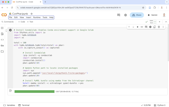
Figure 1: Screenshot of the first code block used to set up the Google Colab environment by installing CondaColab. A horizontal blue progress bar appears above the cell during execution and turns green upon successful completion. Please click here to view a larger version of this figure.

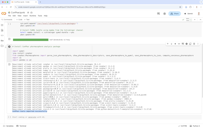
Figure 2: Screenshot of the second code block used to install the ConPhar package in Google Colab. Please click here to view a larger version of this figure.

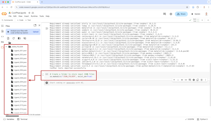
Figure 3: Screenshot showing pharmacophore JSON files successfully uploaded into the designated folder in Google Colab. Please click here to view a larger version of this figure.

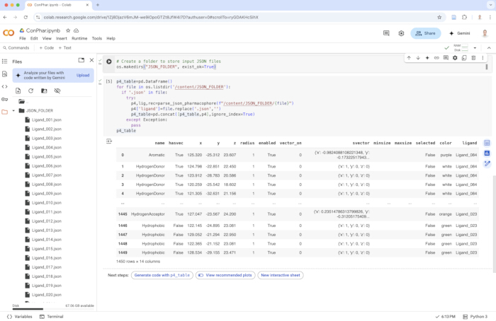
Figure 4: Screenshot showing the code used to extract pharmacophoric features from the JSON files and consolidate them into a single DataFrame. Please click here to view a larger version of this figure.

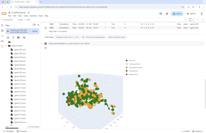
Figure 5: Visualization of the clustering of pharmacophoric features generated during the construction of the consensus pharmacophore model. Please click here to view a larger version of this figure.

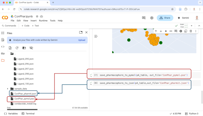
Figure 6: Screenshot showing the successful generation of the consensus pharmacophore files in PyMOL- and Pharmit-compatible formats. Please click here to view a larger version of this figure.

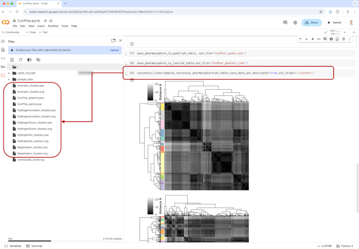
Figure 7: Screenshot showing the generation of consensus pharmacophore files clustered by feature type, including outputs for PyMOL, Pharmit, and dendrogram visualizations. Please click here to view a larger version of this figure.

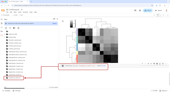
Figure 8: Screenshot showing the successful export of the consensus pharmacophore data to the consensus_result.csv file. Please click here to view a larger version of this figure.

Results

One hundred Mpro complexes co-crystallized with different non-covalent inhibitors were aligned, as exemplified in Figure 9A. Each ligand was then extracted as an individual file (Figure 9B) and subsequently uploaded to the Pharmit server. The session was saved to generate a corresponding JSON file (see Figure 9C).

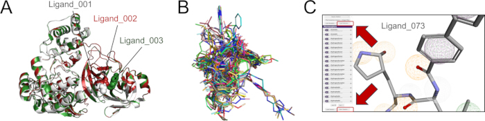
Figure 9: Ligand preparation for consensus pharmacophore modeling. (A) Structural alignment of three representative Mpro complexes co-crystallized with non-covalent inhibitors. (B) Superposition of the 100 ligands included in this study. (C) Upload of each ligand to the Pharmit server using the "Load Features" option, followed by JSON file generation via the "Save Session" option. Both options are indicated with red arrows. Please click here to view a larger version of this figure.

The complete set of JSON files was used to generate the consensus pharmacophore model, which comprised 1450 pharmacophoric features grouped into 110 clusters: 23 aromatic (Aro), 30 hydrogen bond acceptor (HBA), 16 hydrogen bond donor (HBD), 36 hydrophobic (Hyd), and 5 negatively charged (Anion) clusters (Figure 10A, Supplementary Table 1). We identified the larger clusters for each feature for their incorporation into the consensus model. Among the Aro clusters, we selected those with more than 20 elements. From the HBA, HBD and Hyd groups, we retained clusters with at least 50 elements. None of the Anion clusters had more than 4 members, so they were excluded from the consensus model (Figure 10B). These numerical thresholds (>20 members for Aro; ≥50 for HBA, HBD, and Hyd) were empirically defined based on the distribution of cluster sizes to prioritize the most conserved and densely populated interaction patterns.

Figure 10: Clustering of pharmacophoric features from 100 Mpro-ligand complexes. (A) Distribution of 1450 pharmacophoric features: aromatic (Aro) in purple, hydrogen bond acceptor (HBA) in orange, hydrogen bond donor (HBD) in white, hydrophobic (Hyd) in green, and negatively charged (Anion) in red. (B) Clusters containing ≥10 members are shown for Aro, HBA, HBD, and Hyd; all Anion clusters are displayed. The largest clusters-defined as those with ≥20 members for Aro, and ≥50 members for HBA, HBD, and Hyd, and ≥4 members for Anion-are highlighted with dotted spheres. The number of members in each of the largest clusters is explicitly indicated. Please click here to view a larger version of this figure.

Thus, our consensus pharmacophore model included 11 features: 3 aromatic (Aro) features, Aro 1, 2, and 3, derived from clusters with 20, 24, and 45 members, respectively; 4 hydrogen bond acceptors (HBA), HBA 1, 2, 3, and 4, from clusters with 51, 55, 77, and 81 members, respectively; 2 hydrogen bond donors (HBD) from clusters with 51 and 71 members, respectively; and 2 hydrophobic (Hyd) features from clusters with 50 and 52 members, respectively (see Figure 11A).

The pharmacophore model was used to search the PubChem database using the strategy previously reported¹⁰, but no matches were found. To increase search flexibility, the aromatic feature Aro 1 -derived from the smallest and least representative cluster- was removed. This adjustment led to the identification of two hits, including a conformer of the compound with PubChem CIDs 101267741, and 10285538 (see Figure 11B). The 2D chemical structure of compound 101267741 is shown in Figure 11C. Interestingly, this identified compound fits well within the Mpro binding pocket. A comparative analysis with the co-crystallized ligand 38a¹⁵(PDB ID: 9HAJ) shows that the pharmacophore-matching conformer of 101267741 is buried even deeper than 38a within the S1 and S2 subpockets of Mpro. However, 38a occupies a broader region of the pocket, mainly due to its ethyl carboxamide side chain, which extends toward the S1′ pocket. Nevertheless, the key intermolecular interactions of 38a involve other moieties rather than this side chain. In contrast, compound 101267741 forms 11 intermolecular interactions, including seven hydrogen bonds and four hydrophobic contacts. Compared to the three hydrogen bonds and two hydrophobic interactions formed by 38a, the binding mode of compound 101 appears stronger (Figure 11D).

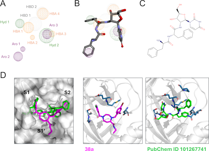
Figure 11: Pharmacophore search in the PubChem database. (A) The complete consensus pharmacophore model contains 11 features: 3 aromatic (purple), 4 hydrogen bond acceptors (orange), 2 hydrogen bond donors (white), and 2 hydrophobic (green). (B) The conformer of compound PubChem 101267741 aligned with the reduced pharmacophore model after removal of the Aro 1 feature, and (C) Two-dimensional chemical structure of compound identified. (D) Comparative analysis of the binding modes of compound 38a (magenta; from PDB ID: 9HAJ) and compound PubChem CID 101267741 (green) to SARS-CoV-2 Mpro catalytic pocket. The corresponding intermolecular interactions for each compound are shown on the right. Hydrogen bonds and hydrophobic interactions are shown as dashed lines in blue and gray, respectively. Please click here to view a larger version of this figure.

Supporting File 1: Pharmacophore workflow script. Please click here to download this File.

Supporting Table 1: Clustering Summary of Pharmacophoric Features. Number of Clusters, Members per Cluster, Centroid Coordinates, and Cluster Radii Please click here to download this File.

Discussion

Pharmacophore modeling aids rational drug discovery¹⁶. The protocol described in detail here was employed for the generation of a consensus pharmacophore for the SARS-CoV-2 main protease (Mpro) starting from dozens of non-covalent inhibitors, but it can be applied to any biological target with known ligand-bound conformations, especially those with extensive ligand datasets. Compared to individual pharmacophore or purely ligand-based models, this consensus approach enhances robustness and reduces bias by integrating multiple ligand conformations. The consensus pharmacophore model generated by this protocol can be applied to diverse molecular libraries, including public databases such as ChEMBL¹⁷and ZINC¹⁴, commercial collections, and proprietary in-house compound libraries. This versatility enables the exploration of broad and diverse chemical spaces in virtual screening campaigns, thereby increasing the likelihood of identifying novel bioactive compounds. Thus, this workflow supports the identification of novel bioactive compounds with the desired interaction profiles.

One critical step in this protocol involves accurate preparation and alignment of ligand-target complexes. Precise pre-alignment of ligands in their bioactive conformations is essential to ensure meaningful and reliable integration of features, as misalignment can weaken model predictive power¹⁰. To achieve optimal alignment, we recommend performing structural superposition using conserved protein binding site residues or backbone atoms. For datasets with diverse ligands, aligning key interaction points or pharmacophoric features enhances consistency across the set. Additionally, careful manual inspection and correction of outlier ligand conformations are advised to prevent artifacts that could diminish model accuracy. In addition, the open-source nature of ConPhar facilitates integration into other computational workflows as well as advanced adjustments in the clustering parameters. Experienced users may modify the clustering parameters of pharmacophoric features to get a balance between model generality and specificity. Those modifications can be directed by ligand dataset size, chemical diversity, or target complexity. For example, when dealing with highly diverse ligands, stepwise clustering or subgroup analysis can better capture relevant features¹⁸.

The ConPhar tool is currently under active development. This offers significant flexibility for users wishing to tailor the tool to specific research needs, including integration with complementary software pipelines. However, because the software may still undergo changes, users are encouraged to monitor official updates and consult version-specific documentation. Reporting encountered issues will contribute to its continued improvement and broader community validation. Our protocol will build models with comprehensive interaction patterns, and thus, they can be employed in virtual screening of large libraries. In our representative results, we employed the obtained pharmacophore in the identification of two new potential ligands for the catalytic region of Mpro. Ultimately, this consensus pharmacophore method streamlines hit identification and accelerates lead optimization.

However, we identify the following limitations of the protocol: i) dependence on high-quality ligand-bound structures, since low-resolution data can reduce model accuracy; ii) the risk of overlook unique and important interactions crucial for specific ligands, since the consensus pharmacophore emphasize shared features; and iii) the reproducibility can be affected by different feature definition across different software tools¹⁹. However, these limitations can be overcome by refining the structure of a protein-ligand system by molecular dynamics simulations²⁰, cluster retention based on user knowledge, and consistent use of software for identification of pharmacophoric features.

Although the consensus pharmacophore model in this protocol was not validated using classical binary metrics, its predictive capacity has been demonstrated in a previous study¹⁰. In that work, an independent test set of 78 chemically diverse ligands was used to validate a consensus pharmacophore generated with the same methodology. The validation set included ligands with ≤0.5 Tanimoto similarity, molecular masses between 200 and 700 g/mol, ≤17 rotatable bonds, and at least three pharmacophoric features. The model successfully identified known actives, supporting its applicability in virtual screening workflows and its robustness across chemically diverse candidates.

The protocol reported here enables the construction of pharmacophore models that capture comprehensive interaction patterns characteristic of the target. This is particularly valuable for targets with extensive ligand data, such as viral proteases, kinases, and nuclear receptors²¹. The generated models are suitable for virtual screening of large compound libraries, facilitating the identification of novel bioactive candidates. By highlighting conserved and functionally relevant features, the consensus pharmacophore approach supports both early-stage hit discovery and subsequent lead optimization.

Materials

List of materials used in this article

Name	Company	Catalog Number	Comments
Google Colab	Google LLC	https://colab.google	Web-based platform for running Python notebooks; used here to execute ConPhar and PyMOL scripts for consensus pharmacophore modeling.
Pharmit	Koes Lab at the University of Pittsburgh	https://pharmit.csb.pitt.edu/search.html	Web platform for interactive pharmacophore virtual screening and chemical space exploration, allowing upload of ligand files and generation of pharmacophore features
PyMOL	Schrödinger, Inc.	https://www.pymol.org	Molecular visualization and structural alignment software used for protein–ligand complex superposition and analysis
Supporting File 1 Pharmacophore Workflow Script	Google LLC	https://colab.research.google.com/drive/1Zj8DjazV6mJM-we9iOpoGTZt8JfW4I7D?usp=sharing	Full executable script for installing Conda, PyMOL, and running the pharmacophore workflow in Google Colab. Also provided as Supporting File 1.

References

- Leach, A. R., Gillet, V. J., Lewis, R. A., Taylor, R. Three-dimensional pharmacophore methods in drug discovery. J Med Chem. 53 (2), 539-558 (2010).
- Giordano, D., Biancaniello, C., Argenio, M. A., Facchiano, A. Drug design by pharmacophore and virtual screening approach. Pharmaceuticals (Basel). 15 (5), 646(2022).
- Schaller, D., et al. Next generation 3D pharmacophore modeling. WIREs Comput Mol Sci. 10 (4), e1468(2020).
- Wolber, G., Langer, T. LigandScout: 3-D pharmacophores derived from protein-bound ligands and their use as virtual screening filters. J Chem Inf Model. 45 (1), 160-169 (2005).
- Ekins, S., Mestres, J., Testa, B. In silico pharmacology for drug discovery: Methods for virtual ligand screening and profiling. Br J Pharmacol. 152 (1), 9-20 (2007).
- Wolber, G., Dornhofer, A. A., Langer, T. Efficient overlay of small organic molecules using 3D pharmacophores. J Comput Aided Mol. 20 (12), 773-788 (2006).
- Schuster, D. 3D pharmacophores as tools for activity profiling. Drug Discov Today Technol. 7 (4), e205-e211 (2010).
- Qing, X., et al. Pharmacophore modeling: advances, limitations, and current utility in drug discovery. J Recept Ligand Channel Res. 7, 81-92 (2014).
- Ullrich, S., Nitsche, C. The SARS-CoV-2 main protease as drug target. Bioorg Med Chem Lett. 30 (17), 127377(2020).
- Ruiz-Moreno, A. J., et al. Consensus pharmacophore strategy for identifying novel SARS-CoV-2 Mpro inhibitors from large chemical libraries. J Chem Inf Model. 64 (6), 1984-1995 (2024).
- Schrödinger, L., DeLano, W. PyMOL, 2020. , http://www.pymol.org/pymol (2020).
- Sunseri, J., Koes, D. R. Pharmit: Interactive exploration of chemical space. Nucleic Acids Res. 44 (W1), W442-W448 (2016).
- Kim, S., et al. PubChem 2025 update. Nucleic Acids Res. 53 (D1), D1516-D1525 (2025).
- Tingle, B. I., et al. ZINC-22: A free multi-billion-scale database of tangible compounds for ligand discovery. J Chem Inf Model. 63 (4), 1166-1176 (2023).
- Hazemann, J., et al. Accelerating the hit-to-lead optimization of a SARS-CoV-2 Mpro inhibitor series by combining high-throughput medicinal chemistry and computational simulations. J Med Chem. 68 (8), 8269-8294 (2025).
- Momin, Y., Beloshe, V. Pharmacophore modeling in drug design. Adv Pharmacol. 103, 313-324 (2025).
- Zdrazil, B., et al. The ChEMBL database in 2023: A drug discovery platform spanning multiple bioactivity data types and time periods. Nucleic Acids Res. 52 (D1), D1180-D1192 (2024).
- Zhou, L., Griffith, R., Gaeta, B. Combining spatial and chemical information for clustering pharmacophores. BMC Bioinformatics. 15 (Suppl 16), S5(2014).
- Guner, O. History and evolution of the pharmacophore concept in computer-aided drug design. Curr Top Med Chem. 2 (12), 1321-1332 (2002).
- Wieder, M., Perricone, U., Seidel, T., Boresch, S., Langer, T. Comparing pharmacophore models derived from crystal structures and from molecular dynamics simulations. Monatsh Chem. 147 (3), 553-563 (2016).
- Santos, R., et al. A comprehensive map of molecular drug targets. Nat Rev Drug Discov. 16 (1), 19-34 (2017).
Reprints and Permissions