Age-dependent Dynamics of Locomotion in Caenorhabditis elegans: A Lyapunov Exponent Analysis

Summary

This study examines the effect of age on locomotion in C. elegans by measuring the largest Lyapunov exponent (LLE). As they age, C. elegans show an increase and subsequent decline in motor control. Results show a peak LLE at five days, followed by a decline as the worms age.

Abstract

This study investigates the influence of age on the mobility of Caenorhabditis elegans (C. elegans) by employing Dynamic Optical Diffraction (DOD) to estimate the Largest Lyapunov Exponent (LLE). The LLE, a key metric in dynamical systems, quantifies the rate of divergence or convergence of trajectories in phase space, indicating the predictability and chaos in the system's dynamics, in this case, the locomotive behaviors of the worm. 632 nm laser light diffracts off the swimming worm in a water column, forming a diffraction pattern. A photodiode detects the light at a single point within the diffraction pattern, capturing a one-dimensional time series as the worm undulates. This time series serves as a composite representation of the entire worm's motion, encapsulating its locomotion dynamics since one point in the diffraction pattern is a superposition of all points on the worm. The time series is then embedded into a higher-dimensional phase space to calculate the LLE. C. elegans typically live for around 14 days, following a pattern of increasing and declining motor control with age. To isolate age-specific effects, worms were transferred to fresh agar plates containing E. coli every two days, ensuring they were appropriately aged (3 to 12 days old). Analysis of a cohort of 13 C. elegans revealed that the LLE peaked at five days post-hatching, at a rate of 1.34 ± 0.03 1/s. This peak signifies a critical point in development where the worms' locomotion displays the highest complexity and chaotic behavior. The observed LLE values align with the Moore equation, a well-established model that describes age-related changes in voluntary activity, linking decreasing motor control and activity levels with increasing age in C. elegans.

Introduction

The locomotion of Caenorhabditis elegans (C. elegans), a microscopic worm, has been studied to further the understanding of the wiring of motor neurons because this nematode is neurologically simple, with only 302 neurons¹. C. elegans is a model organism that is easily maintained with a life span of only 14 days². Only around 72 neurons of 302 in C. elegans are used for locomotion and are located throughout the nematode's adult body¹. The low-dimensional movement (i.e., side-to-side, forward, and backward)³ of C. elegans makes them an easy specimen from which to track ranges in LLE. The nervous systems of nematodes are understood to an incredible extent⁴.

Video analysis has helped quantify C. elegans locomotion by measuring quantities such as radius of curvature, undulation frequencies, and wavelength⁵. These measurements have established control variables that enable the comparison of locomotory properties in different environments and under various conditions^6,7. This information forms an evolving model of the circuitry driving the locomotion of C. elegans⁸ and even enables the creation of virtual as well as physical dynamic simulations of worms⁹.

Dynamic Optical Diffraction (DOD)¹⁰ has also been used to quantify the locomotion of C. elegans. During DOD, low-intensity laser light bends around the live worm, forming a far-field diffraction pattern known as a Fraunhofer diffraction pattern. The intensity distribution in the live pattern changes as the nematode moves. One point in the diffraction is a superposition of all points on the worm, so that the time-dependent intensity in the diffraction pattern forms a one-dimensional time series containing information about the locomotory dynamics¹¹. We focus on the age-dependent Largest Lyapunov Exponent (LLE) of locomotion that we calculate from the experimental one-dimensional time series. The LLE at different developmental stages is comparable to other age-related studies, showing that the neural circuitry manifests in locomotory patterns that can be measured using various tools, such as video analysis or DOD⁵.

DOD provides a time series sensitive on multiple scales since the interference pattern can resolve the locomotion to a fraction of the wavelength used while also accounting for large-scale changes in the species' plasticity (shape). This feature is particularly useful when a system is sensitive to initial conditions, as in chaotic systems where small changes lead to exponential changes in the trajectory, also known as the butterfly effect¹². For this reason, it is crucial to capture the time series at a rate that allows for the recording of small changes, as these changes can result in significant shifts as the system evolves. A photodiode (PD) can capture the time series faster than many expensive high-speed cameras. The combination of the spatial sensitivity in the diffraction pattern and a high data accumulation rate can capture the essence of a chaotic system^13,14.

The LLE describes the exponential divergence of phase space trajectories. The phase space contains all possible states of a system, described by their state variables (or coordinates) and their associated derivatives (or momenta)¹⁵. Different trajectories describe the evolution of the system for different initial conditions. In a chaotic system, two nearby trajectories will diverge exponentially over time, and that divergence is quantified by a positive LLE. In physical systems, this divergence manifests as the propagation of uncertainty in the system's initial conditions, and also as the inability to reliably predict the system's state after some time, as given by the LLE¹⁴.

In experimental systems, the state variables are often unknown; however, the topology of the phase space can be reconstructed from only one measured variable using Takens embedding theorem¹⁶ by constructing its time-delayed versions (equivalent to time derivatives). Each time-delayed version is represented on an axis; together, the time delays form a lag plot, which is topologically identical to a phase plot if the time series is infinitely long. Experimental time series are limited in length and, therefore, can only render estimated LLEs that are bounded by experimental uncertainties.

The locomotion of C. elegans carries a positive LLE¹⁰, an indicator of chaos. A young organism undergoes locomotory changes with age¹⁷. A larger LLE indicates a lower predictability in comparison to a smaller LLE. The LLE provides a reliable method for quantifying an organism's locomotory patterns^10,13,14. Nematode locomotory characteristics are related to the neurons within the nematodes¹⁸. According to Cohen et al.¹⁹, nematode locomotion is dependent on motor neurons, suggesting that the study of complexity in the nematode's locomotion is also related to its neuronal circuitry.

We calibrate the LLE based on age to minimize uncertainties for future studies. Past studies averaged the LLE in three to six-day-old nematodes¹³. This study carefully monitored nematodes' ages to facilitate a rigorous analysis of declines associated with aging. Additionally, changes in locomotion have been investigated to identify other biological alterations in C. elegans¹⁸. Moore's equation tracks age parameters related to locomotion²⁰. Here, we use a modified version of Moore's equation that allows for flexibility in when the locomotory mechanism is in place to be evaluated, introduced as a temporal marker T:

, (1)

where P(t) represents performance, t is time, a and c represent scaling parameters, while b and d are the characteristic times of the exponential growth and decline, respectively. Moore's equation has been shown to predict the trajectories of seemingly unrelated quantities, such as speed and voluntary activity, as organisms age. Species can be characterized by the shape of the curve as specified by Moore's equation; i.e., some species may peak sooner than others²¹.

Protocol

1. C. elegans preparation for data acquisition

1. Put 0.5 mL of E. coli with OD600 in each Nematode Growth Medium (NGM) agar plate for the nematodes to eat. Wait for the E. coli to dry on each plate of agar.
2. Acquire a control plate of C. elegans from any biological materials supplier in order to make new plates of C. elegans for the purpose of age control.
3. Sterilize a platinum pick using a flame from a Bunsen burner or equivalent. Use a dissecting microscope to pick 5-10 adult wild-type C. elegans to put into each plate.
4. Allow the nematodes to lay eggs for 4-5 h before picking the adults from the plate. Incubate the remaining nematodes and allow them to pick them on the desired day.
5. On the day of data collection, fill an optical grade quartz cuvette of 4.5 mL with dimensions 10 mm x 10 mm x 45 mm with room temperature distilled water just below the top of the cuvette to prevent any spillage when a plastic top is added. Pick 2-3 nematodes and gently place them into the cuvette. Once the nematodes are in the cuvette, place it on its side to easily align the worm in the laser beam. The C. elegans may float towards the bottom but will continue with swimming undulations as long as it is fully immersed in water⁵.

2. Data collection

NOTE: The procedure below for recording the time series must be implemented around the same time each day to minimize uncertainties in age.

1. Set up the experiment described in the previous article²². Implement a small modification of building a periscope with two mirrors and placing the cuvette on its side between the two mirrors to make it easier to center the worm in the laser beam later. Instead of the camera, place a PD in the diffraction pattern (Figure 1).
   1. Align the mirrors vertically to build the aforementioned periscope.
      NOTE: This is the only laser alignment work that needs to be completed.
2. Turn on the HeNe (Helium Neon) laser and let it warm up to reach thermal equilibrium (~15 min).
3. Initiate the digital oscilloscope to begin data collection. Set the parameters of the time interval and memory buffer on the digital oscilloscope. Set the time interval to 100 s and implement a memory buffer of at least 100 kilosamples per second (kS).
4. Set the resolution to 1 kHz for the data acquisition rate and 12 bits to resolve the amplitudes, which helps distinguish complexity at small scales²³.
5. Set the oscilloscope to center the intensity oscillations by using the Auto AC offset to center the time series at zero volts.
6. Pick 2-3 nematodes and place gently into a cuvette filled with distilled water so that it will be easier to find and center at least 1 worm in the laser beam. Do not shake the cuvette.
7. Place the cuvette holding 2-3 nematodes in the periscope and center 1 nematode in the laser beam.
   1. When the C. elegans is centered in the laser beam, a far-field diffraction pattern will form about 50 cm from the periscope.
8. Place the photodiode in the far-field diffraction pattern when a C. elegans traverses the laser beam. Ensure the PD is positioned off-center in the diffraction pattern to capture diffracted light rather than the central maximum (transmitted laser beam).
9. Collect at least 10 s of data to calculate the LLE reliably; i.e., at least 10,000 data points are required to calculate a stable LLE.
   NOTE: Fewer data points result in an LLE that artificially fluctuates.
10. Repeat the above data collection for each day 9-15 times. Collect data for ages 3-12 days at the same time of day.

3. Data analysis

NOTE: For the data analysis, the time series is embedded in phase space using a lag plot¹⁶ and then estimate the LLE by calculating the divergence of the trajectories.

1. Choose sections in the time series when the nematode swims freely inside the laser beam by carefully examining the time series. Figure 2A shows a viable time series with a continuous signal of at least 20 s.
2. Screen the time series for a low signal-to-noise ratio (Figure 2B). Establish the noise level by recording a time series without the worm in the cuvette. The features in the time series, not just the amplitude, must be more than twice the noise level.
3. Exclude any saturated data from the relevant time series (Figure 2C). If too much data is saturated to extract useful information, return to the Data Collection section above, repeat steps 2.7.1 through 2.9, and adjust the intensity level by moving the photodiode away from the central maximum.
4. Determine the mean frequency given by
      (2)
   where f is the frequency and P is the power spectrum (Figure 3). This can be done computationally using a Fast Fourier Transform (FFT) and then averaging the frequencies. Many computational programs have a built-in function to calculate the mean frequency of a data set.
5. Reconstruct the topology of phase space using a time delay method. Choose a time series X and delay the time series by a time delay τ to resolve the trajectories (Figure 4). The optimal time delay is determined by identifying the first local minimum in the mutual information (MI)²⁴:
       (3)
   where N is the number of points, X_i is a point in the time series X, while X_i+τ is a time-delayed point in the same time series. p(X_i) is the probability of point X_i occurring, and p(X_i+τ) is the probability of X_i+τ occurring. p(X_i, X_i+τ) is the joint probability²⁵ of both the time series X_i and the lagged time series X_i+τ coinciding.
6. Identify the first minimum in the MI graph between 0.140 and 0.240 s (140 and 240 datapoints), as shown in Figure 5. There is no exact number for the lag; the primary purpose is to resolve the phase trajectories enough to determine the divergence.
7. Use the time series X_i and its lagged versions by τ, as determined by minimizing the MI in the previous step.
8. Determine the embedding dimension. The most suitable embedding dimension is the lowest dimension for which false nearest neighbors (FNN) stabilize at a minimum (Figure 6)²⁶. Use the method developed by Abarbanel et al.^27,28.
9. Use the Rosenstein algorithm²⁹ to reconstruct the dynamic system in a phase space and track the divergence of nearby trajectories over time. In particular, utilize the MATLAB routine by Merve Kizilkaya, as posted on the MATLAB forum³⁰, to calculate the LLE. This routine requires the following input: the time series, mean frequency of the attractor, the time lag τ, the data acquisition rate for the time series, and the interval to fit the divergence.
10. Repeat the above procedure for 9-15 datasets to reduce the uncertainty of the LLE estimates. Average the LLEs for each day and then fit Moore's curve (Figure 7).

Results

While measuring the LLE versus age, we also measured other quantities often associated with complex dynamic systems, such as the frequency of the attractor, MI, and FNN. We collected age-study data from days 3 to 12. The worms are too small and immature before they are 3 days old to handle manually. At 12 days, the worms are aged and barely move since their neuronal circuits deteriorate and their nervous system declines³¹.

The Rosenstein algorithm selects a neighboring point at an interval of at least one mean period for every point on the embedded trajectory. Starting with the separation vector between the two points on the two neighboring trajectories (Figure 8), the algorithm tracks the evolution of the divergence. The separation of the trajectories initially increases exponentially due to the chaotic nature of the system³², and then it plateaus since the trajectory is bounded. Plotting the logarithm of the average divergence over time tracks the separation of the trajectories (Figure 8 and Figure 9). The slope of the linear least-squares fit to the first part of the curve before it flattens out results in a reliable estimate for the system's LLE³³. Note that uncertainty is involved in choosing the range for the least-squares fit and the fit itself. The sensitivity to initial conditions causes the linear fit region to display an oscillatory behavior as the divergence is tracked on the attractor. The biological variation between worms, which were averaged for each age group, outweighs the variability in the linear LLE fit for a single trial, as shown in a previous publication¹⁰.

The time series (Figure 2A) shows that peaks and troughs coincide with the aspects of the worm's locomotion, such as changes in swimming frequency, shape, and orientation. The time series is aperiodic; the oscillations in the time series never repeat, yet remain bounded in intensity. The frequency is steady while fluctuating slightly, indicating complexity and boundedness in frequency. Figure 10 shows a declining trend in swimming frequencies as the worm ages, which breaks down on day 12. The mean frequency jumps after day 12 for most worms. This is likely an indication of the neural circuit breaking down. In contrast, the average lag τ, as determined by the first minimum of the MI, increases as the population ages, since the cycle elongates (Figure 11).

In our case, the MI represents the statistical overlap between two lagged time series. If the MI is minimal, then there is minimal overlap between trajectories. Theoretically, chaotic trajectories never overlap; however, in practice, with limited significant digits and some experimental noise, some points will overlap within some tolerance²⁴. We aim to minimize the possibility of overlap by minimizing the MI. The difference between a minimized MI and a significantly larger MI is illustrated in Figure 4.

The embedding dimension is determined by the false nearest neighbors (FNNs). The number of FNNs flattens with 5% or fewer FNNs around embedding dimensions 3 or 4. In Figure 6, the age of the nematodes does not affect the embedding dimension, except on day 12, when the worm is almost at the end of its lifespan.

The trajectory of the LLE follows Moore's curve (Figure 7) with a peak at 5 days, indicating that the most unpredictable (and possibly complex) locomotion occurs when the C. elegans are newly mature. In Figure 7, a graph of LLEs from days 3 through 12 shows a linear increase with a peak at 5 days, followed by a decrease after day 5. The error bars in Figure 10 represent the standard deviation of the mean^4,34 and reflect several factors, including the diversity within biological species and the LLE estimation. The variation between the worms tends to outweigh the uncertainties in the LLE fitting routine. The variability between days, like days 5 and 7, does not overlap, so the data is clearly distinguishable. The trend of LLEs with age closely matches a Moore's equation from a previous study¹⁸, which describes age effects on memory and locomotion in other living organisms.

The LLEs in Table 1 are consistent, showing a slowly increasing and then decreasing trend with age. The values are consistent with previously published results using DOD¹⁰ and video analysis^34,35.

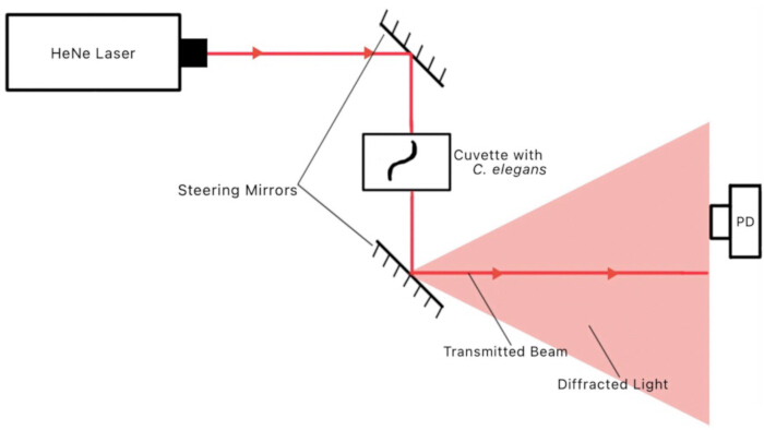
Figure 1: Experimental far-field diffraction setup (not drawn to scale). The steering mirrors form a periscope. The cuvette containing the C. elegans is placed between the steering mirrors. The laser beam is diffracted by the worm and travels towards the PD via the second steering mirror. Please click here to view a larger version of this figure.

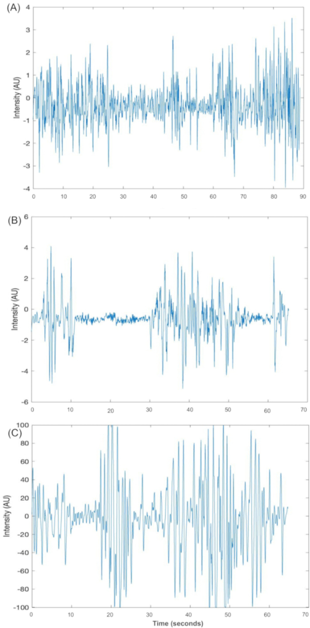
Figure 2: Intensity time series. The DOD time series shows intensity fluctuations as the nematode moves in the laser beam with (A) a viable time series for data analysis. (B) This time series indicates that the interval between 11 and 30 s exhibits no signal; it merely displays the system's noise level, as the shorter steady amplitudes primarily originate from scattered light. (C) This time series has a few instances of saturated data. Each data point represents a significant spike in the graph that is cut off and flattened at the peaks and troughs. In this example, the spikes become flattened as the intensity ranges from -100 to 100 AU between 45 and 50 s. Please click here to view a larger version of this figure.

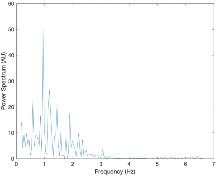
Figure 3: Power spectrum. The power spectrum shows a maximum at around 0.95 Hz. The frequencies are spread out since the frequency in the trajectories on the attractor shifts and never exactly repeats. Please click here to view a larger version of this figure.

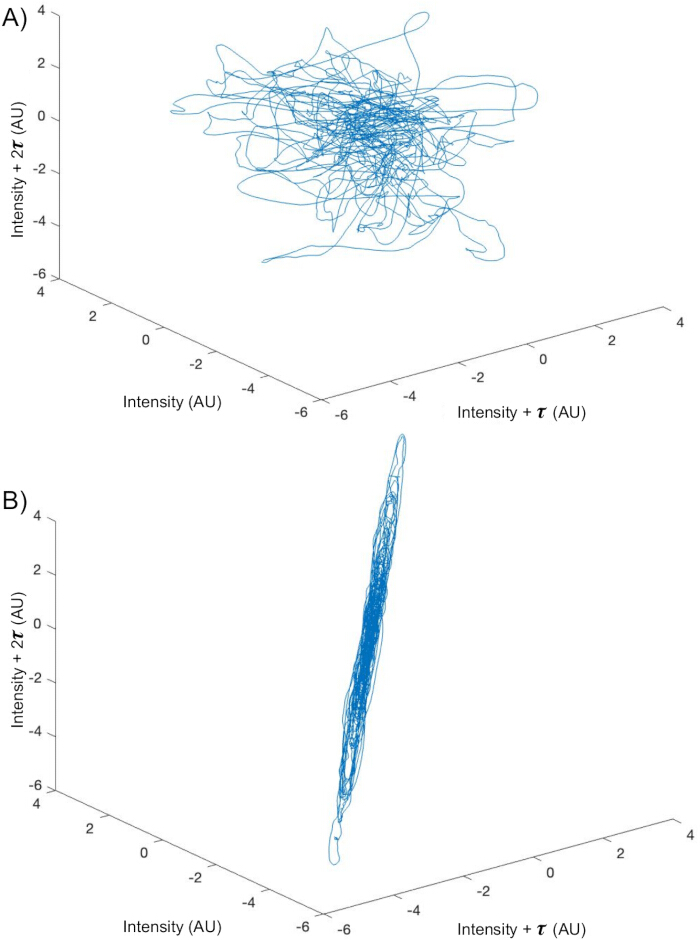
Figure 4: Experimental data embedded in 3D lag plots with two different lags of the same time series of a 9-day-old worm. This time series shows that locomotion is a bounded attractor consistent with chaos theory. (A) The trajectory is resolved using the first local minimum (MI ≈ 2.11), giving a lag of around 0.183 s (183 datapoints). The visible trajectory crossings are a result of a projection onto a two-dimensional space. (B) This lag plot remains unresolved by an inappropriate lag of 0.002 s (2 datapoints, (MI > 7)) as the points are too close together to be distinguishable and do not show divergence. Please click here to view a larger version of this figure.

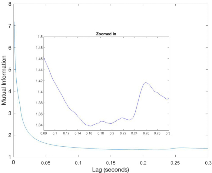
Figure 5: The exponential decrease of the mutual information. The first minimum in the MI determines the lag of the dataset at 0.161 s (161 datapoints) in this specific case to resolve the phase trajectory. This lag shifts the time series value to reconstruct the attractor in phase space. The lag only needs to be near the first minimum, enough to resolve the trajectories. Please click here to view a larger version of this figure.

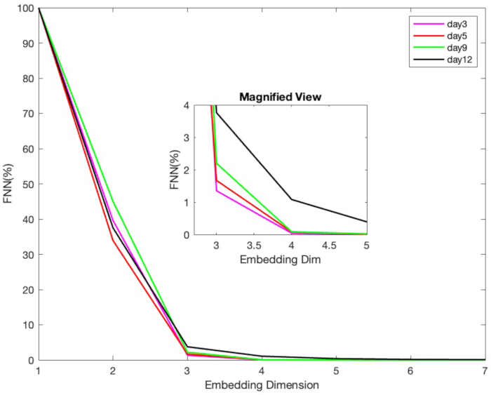
Figure 6: The average embedding dimensions on days 3, 5, 9, and 12, respectively. A magnified view of the embedding dimension is used to show the specific difference between the embedding dimensions of each day. Only day 12 displays a notable difference. Please click here to view a larger version of this figure.

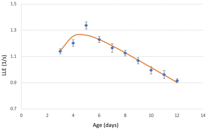
Figure 7: The average of the estimated LLEs between days 3 and 12. The LLE peaks at 5 days. For up to 5 days, nematodes exhibit a growth trajectory consistent with the transition from immaturity to maturity. After those 5 days, nematodes experience a decline in divergence. The uncertainties are measures of the standard deviation of the mean, which is dominated by variations between worms. Please click here to view a larger version of this figure.

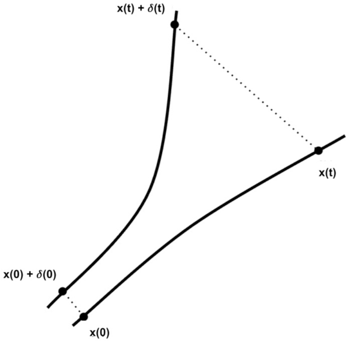
Figure 8: Depiction of the divergence present in chaos theory. A positive LLE will cause initially close trajectories to diverge over time. t is a time interval, d is the divergence, and x(t) is a point in phase space. Please click here to view a larger version of this figure.

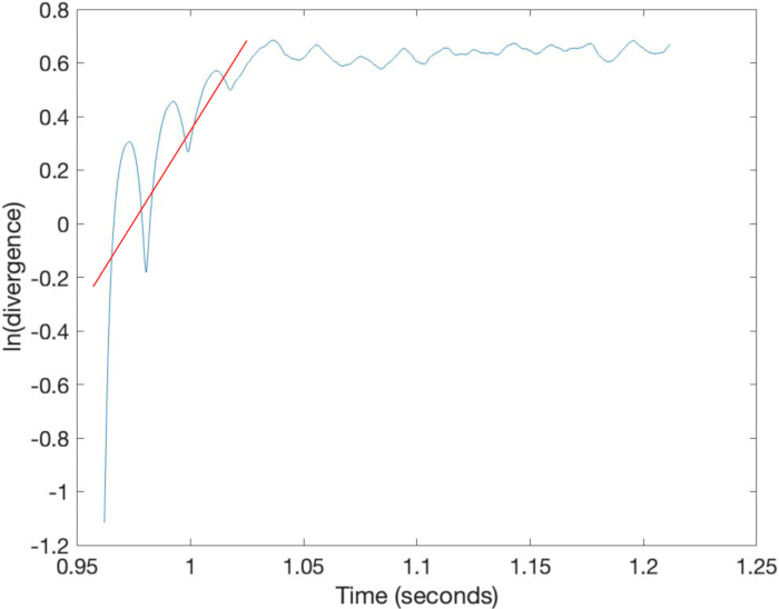
Figure 9: Phase trajectory divergence on a logarithmic scale. The estimated LLE is the slope of the linear fit (1.08 1/s) in the rising region before flattening out due to the boundedness of the attractor between 0.96 and 1.01 s. Please click here to view a larger version of this figure.

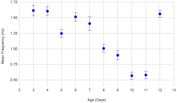
Figure 10: The average mean frequency for each day. Day 12 average denotes a significant change in the neurological signals driving locomotion. Please click here to view a larger version of this figure.

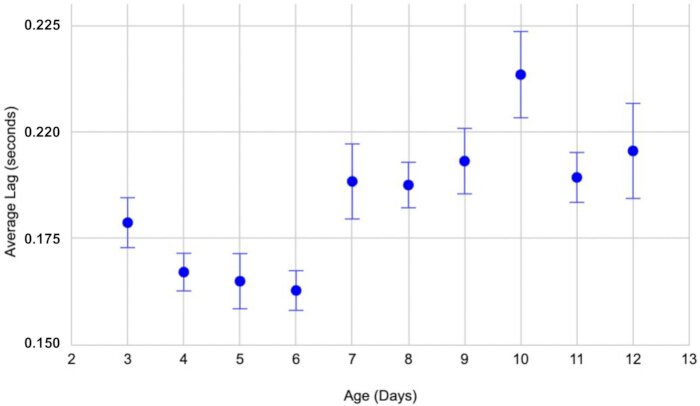
Figure 11: The average lag for each day. The MI leads on average to lower lags between days 3 and 6, while a higher average lag appears between days 7 and 12. Please click here to view a larger version of this figure.

Age (days)	Number of Datasets	LLE (1/s)	Standard Deviation of the Mean (1/s)
3	11	1.14	0.02
4	15	1.20	0.03
5	13	1.34	0.03
6	11	1.23	0.02
7	10	1.16	0.03
8	12	1.13	0.02
9	12	1.07	0.02
10	9	1.00	0.03
11	9	0.96	0.03
12	9	0.92	0.02

Table 1: The number of datasets and average LLE for each day of the age study. The LLEs are consistent with previous data collected through DOD and show the increasing then decreasing trajectory of the Moore's curve from Figure 7. 9-15 datasets were collected for each day of data. The datasets trended down as the worms got older due to the nature of their muscle degradation and neuronal decline, causing decreased locomotion.

Discussion

We categorized C. elegans locomotion by evaluating the LLE across different ages, supported by parameters such as swimming frequency, mutual information (MI), and false nearest neighbors (FNN)-each of which offers additional insight into the system's dynamical properties. The deterministic and non-linear properties of this system are studied using surrogate data methods and recurrence plots³⁶.

Using DOD to quantify the effects of aging on locomotion is a complementary technique to traditional microscopy. It is not a substitute for visually inspecting the microscopic species; it provides a consistent and efficient way to quantify locomotion beyond traditional techniques. Since DOD bypasses video analysis, a portion of the computational workload is inherently managed by the optical technique, as diffraction directly maps the intensity distribution into Fourier space. The superposition of the optical field during diffraction tracks the entire microscopic species. Ideally, the resolution is governed by the wavelength λ of the light used, in this case, 632 nm. Even a shift of a fraction of the wavelength will result in a change in the intensity. For this reason, the resolution is governed by the range and resolution of the photodetector as well as the power of the laser. For example, if the detector senses a time series signal that fluctuates between two voltages, Vmin and Vmax, and the resolution is n bits (see Protocol step 2.4), then the maximum resolution is λ/n, or in our case, 632 nm/12. In theory, this method can be applied to any body that changes its shape; however, DOD is particularly well-suited for microscopic species, as inexpensive lasers with the appropriate wavelengths are readily available and cost-effective.

To ensure a clear and consistent diffraction pattern, the worm must be carefully tracked and kept centered within the laser beam as it swims. If the worm drifts out of alignment, the signal may degrade or be lost entirely. To mitigate issues of photodiode saturation and reduce stochastic noise, a neutral density filter is used to attenuate the laser intensity. This filtering helps maintain the dynamic range of the photodiode and prevents oversaturation in the recorded time series. Nonetheless, any segments of the data exhibiting excessive saturation or low signal-to-noise ratios are excluded from the final analysis to maintain data quality.

A drift in swimming frequency produces a continuous frequency spectrum, an established early marker of chaos¹³. The inverse relationship between mean frequency and MI suggests that approximately ⅛ of a cycle resolves the trajectory with sufficient accuracy to estimate the LLE, akin to the resolution required for analyzing a sinusoidal waveform.

The low percentage of FNNs around embedding dimensions 3 and 4 in Figure 6 implies low noise levels in both the C. elegans locomotion and the optical system. However, in 12-day-old worms, the percentage of FNNs increases slightly but remains well below 5%, not necessarily due to a rise in the true embedding dimension, but likely due to increased noise in the locomotor signal, attributed to neural degradation in aging organisms^34,37.

Changes in the LLE throughout development show that the degree of chaos in locomotion varies with age, closely matching predictions from Moore’s equation. A peak in the LLE early in life is consistent with characteristics of R-selected species, such as C. elegans, which must develop neuromuscular functionality rapidly in the absence of parental care. Notably, 70% of long-range neuronal connections are formed when the worm is only 20% of its adult size^37,38. In contrast, K-selected species, such as humans, exhibit slower neurological development, supported by parental investment, resulting in delayed but more complex motor patterns. These differences are reflected in the timing of peak LLE across species.

The short life cycle of C. elegans, approximately 14 days, with rapid development during the first two days over four larval stages², makes it particularly suitable for studying peak complexity in locomotion. While previous studies have focused on neuronal structure decline to explain age-related changes in locomotion^34,39, our work connects these physical changes to the system’s underlying chaotic dynamics. The integration of DOD with nonlinear dynamics enables precise quantitative characterization across multiple length scales, offering new insights into the neuronal drivers of behavior. The consistently positive LLE across developmental stages strongly supports the presence of chaotic behavior in the locomotor system.

This study offers a novel methodological framework for examining age-related behavioral changes in C. elegans, thereby extending the current understanding of the biological and dynamical correlates of motor decline. It further validates the use of the LLE as a sensitive biomarker for age-associated neurological changes and demonstrates that the LLE is a reliable quantitative measure of locomotor dynamics affected by aging.

DOD is a powerful, non-invasive method for quantifying locomotion and chaos in microscopic organisms, best viewed as complementary to video analysis rather than a replacement. In its current implementation, the experiment requires nematodes to be at least three days old, since younger worms are too small to yield reliable diffraction signals. The one-dimensional time series extracted from a single point in the diffraction pattern necessarily compresses spatial information, which can obscure localized dynamics along the organism’s body. Multichannel approaches help address this limitation by verifying parameter consistency across the diffraction field, though subtle spatial heterogeneities may still be overlooked. Accurate estimation of the LLE further depends on obtaining sufficiently long, noise-free time series; practical challenges such as worm movement out of the beam or environmental fluctuations can compromise data quality and reduce confidence in LLE values. As with all experimental methods, measurement noise and subjective decisions during LLE fitting introduce additional uncertainty, which for single measurements typically remains within about 15%.

Future work will focus on measuring the LLE under various experimental conditions, enabling comparisons between modeled and measured LLEs. This will facilitate the development of predictive neurological models that could deepen our understanding of how complex motor control emerges and deteriorates over time. We will also continue to explore the consistency of our findings by exploring other computational methods, such as calculating the Entropy-Complexity plane to again verify the deterministic nature of this biological system⁴⁰.

Materials

List of materials used in this article

Name	Company	Catalog Number	Comments
2 Front Surface Aluminum Mirrors	Thorlabs	PF10-03-F01
632 nm HeNe Laser	Newport	LGX1	Any red light laser
Empty Petri Dish	Carolina	971632	Plastic petri dishes in which we pour the nematode growth agar into
Escherichia coli K12, Living, Bacteriophage Host	Carolina	124500	Used as the food source for the C. elegans; OD600
Leica S9i Microscope	Leica Microsystems	LED2500	Dissecting Microscope
Lighter	Bic Lighters		Any type of sterilization tool used to sterlize the pick before and after picking each worm
MATLAB	MathWorks		Rosenstein Algorithm-Routine on the MATLAB forum made by Merve Kizilkaya
Nematode Growth Agar	Carolina	173520	Prepared Media Bottle, 135 mL
Photodiode	Thorlabs	DET36A	350-1100 nm Si Biased Detector
Picoscope5204	Pico Technology	PP376	PC Oscilloscope www.picotech.com
Platinum Pick			Used to scoop C. elegans; it is a small, handmade pick with a glass handheld piece and a platinum scoop
Quartz Cuvette	Starna Cells	21/G/5	Filled with distilled water ito place C. elegans inside

References

- Zhen, M., Samuel, A. D. C. elegans locomotion: small circuits, complex functions. Curr Opin Neurobiol. 33, 117-126 (2015).
- Corsi, A. K., Wightman, B., Chalfie, M. A transparent window into biology: a primer on Caenorhabditis elegans. WormBook. , http://www.wormbook.org (2015).
- Gjorgjieva, J., Biron, D., Haspel, G. Neurobiology of Caenorhabditis elegans locomotion: where do we stand. Bioscience. 64 (6), 476-486 (2014).
- Boyle, J. H. C. elegans locomotion: an integrated approach. , https://core.ac.uk/download/pdf/43059.pdf (2009).
- Pierce-Shimomura, J. T., et al. Genetic analysis of crawling and swimming locomotory patterns in C. elegans. Proc Natl Acad Sci U S A. 105, 20982-20987 (2008).
- Korta, J., Clark, D. A., Gabel, C. V., Mahadevan, L., Samuel, A. D. T. Mechanosensation and mechanical load modulate the locomotory gait of swimming C. elegans. J Exp Biol. 210 (13), 2383-2389 (2007).
- Edwards, S. L., et al. A novel molecular solution for ultraviolet light detection in Caenorhabditis elegans. PLoS Biol. 6 (8), e198(2008).
- Barbulescu, R., Mestre, G., Oliveira, A. L., Silveira, L. M. Learning the dynamics of realistic models of C. elegans nervous system with recurrent neural networks. Sci Rep. 13 (1), 467(2023).
- Sarma, G. P., et al. OpenWorm: overview and recent advances in integrative biological simulation of Caenorhabditis elegans. Philos Trans R Soc Lond B Biol Sci. 373 (1758), 20170382(2018).
- Zanetti, R. F., Canavan, K. L., Zhang, S. G., Magnes, J. Multichannel measurements of C. elegans largest Lyapunov exponents using optical diffraction. Appl Opt. 62 (29), 7812-7818 (2023).
- Magnes, J., et al. Live C. elegans diffraction at a single point. Open J Biophys. 8, 155-162 (2018).
- Lorenz, E. N. The predictability of hydrodynamic flow. Trans N Y Acad Sci Ser II. 25 (4), 409-432 (1963).
- Magnes, J., et al. Chaotic markers in dynamic diffraction. Appl Opt. 59 (22), 6642-6650 (2020).
- Strogatz, S. H. Nonlinear dynamics and chaos: with applications to physics, biology, chemistry, and engineering. , Westview Press. Boulder, CO. (2001).
- Nolte, D. D. Introduction to modern dynamics: chaos, networks, space and time. , Oxford University Press. Oxford. (2015).
- Takens, F. Detecting strange attractors in turbulence. , Springer. Berlin. (1981).
- Murakami, H., et al. Manipulation of serotonin signal suppresses early phase of behavioral aging in Caenorhabditis elegans. Neurobiol Aging. 29 (7), 1093-1100 (2008).
- Marck, A., et al. Age-related changes in locomotor performance reveal a similar pattern for Caenorhabditis elegans, Mus domesticus, Canis familiaris, Equus caballus, and Homo sapiens. J Gerontol A Biol Sci Med Sci. 72 (4), 455-463 (2017).
- Cohen, N., Sanders, T. Nematode locomotion: dissecting the neuronal-environmental loop. Curr Opin Neurobiol. 25, 99-106 (2014).
- Moore, D. H. A study of age group track and field records to relate age and running speed. Nature. 253 (5489), 264-265 (2020).
- Varier, S., Kaiser, M. Evolution and development of brain networks: from Caenorhabditis elegans to Homo sapiens. Network. 22 (1-4), 143-147 (2011).
- Magnes, J., Susman, K., Eells, R. Quantitative locomotion study of freely swimming micro-organisms using laser diffraction. J Vis Exp. (68), e4412(2012).
- Tzepos, D., Trader, O., Magnes, J. 16th Chaotic Modeling and Simulation International Conference, , https://link.springer.com/book/10.1007/978-3-031-60907-7 (2024).
- Fraser, A., Swinney, H. Independent coordinates for strange attractors from mutual information. Phys Rev A. 33, 1134-1140 (1986).
- Starmer, J. The StatQuest illustrated guide to machine learning!!!: triple bam. , StatQuest Publications. (2022).
- Kizilkaya, M. MATLAB routine. , https://www.mathworks.com/matlabcentral (2020).
- Abarbanel, H. D. I., Kennel, M. B. Local false nearest neighbors and dynamical dimensions from observed chaotic data. Phys Rev E. 47, 3057-3068 (1993).
- Kizilkaya, M. False nearest neighbor algorithm. , https://www.mathworks.com/matlabcentral/fileexchange/37239-minimum-embedding-dimension (2020).
- Rosenstein, M. T., Collins, J. J., De Luca, C. J. A practical method for calculating largest Lyapunov exponents from small data sets. Physica D. 65 (1-2), 117-134 (1993).
- Kizilkaya, M. Largest Lyapunov exponent with Rosenstein's algorithm. , https://www.mathworks.com/matlabcentral/fileexchange/38424-largest-lyapunov-exponent-with-rosenstein-s-algorithm (2020).
- Liu, J., et al. Functional aging in the nervous system contributes to age-dependent motor activity decline in C. elegans. Cell Metab. 18 (3), 392-402 (2013).
- Zhang, S. G., Singhvi, A., Susman, K. M., Hastings, H. M., Magnes, J. Dynamic markers for chaotic motion in C. elegans. Nonlinear Dyn Psychol Life Sci. 26 (1), 21-43 (2022).
- Giordano, N. J., Nakanishi, H. Computational physics. , Upper Saddle River, NJ. (2006).
- Olsen, A., Vantipalli, M. C., Lithgow, G. J. Using Caenorhabditis elegans as a model for aging and age-related diseases. Ann N Y Acad Sci. 1067 (1), 120-128 (2006).
- Ahamed, T., Costa, A. C., Stephens, G. J. Capturing the continuous complexity of behaviour in Caenorhabditis elegans. Nat Phys. 17 (2), 275-283 (2021).
- Kennel, M., Brown, R., Abarbanel, H. Determining embedding dimension for phase-space reconstruction using a geometrical construction. Phys Rev A. 45, 3403-3411 (1992).
- Herndon, L. A., et al. Stochastic and genetic factors influence tissue-specific decline in ageing C. elegans. Nature. 419, 808-814 (2002).
- Rosso, O. A., Larrondo, H. A., Martin, M. T., Plastino, A., Fuentes, M. A. Distinguishing noise from chaos. Phys Rev Lett. 99 (15), 154102(2007).
Reprints and Permissions