A chunked image annotation method based on local features is presented to improve electric bike detection in complex elevator scenarios using the EBike-DET dataset and mainstream object detection models.
A subscription to JoVE is required to view this content. Sign in or start your free trial.
Method Article
Improved Chunked Image Annotation Method for Electric Bikes in Complex Elevator Scenarios Based on Local Features
In This Article
Summary
Abstract
The increasing use of electric bikes (EBikes) in confined environments such as residential elevators has raised serious safety concerns and introduced considerable challenges for automated object detection, particularly due to frequent occlusions. Traditional detection approaches, which rely primarily on holistic annotations, often fail to accurately recognize partially occluded EBikes in visually complex scenes. To overcome these limitations, this study proposes a novel chunked annotation method based on local features, offering a more interpretable annotation strategy. By decomposing an EBike into multiple key regions for independent labeling, the proposed method enables detection models to learn fine-grained structural information, thereby improving robustness in occlusion-heavy conditions. Additionally, a dedicated dataset, EBike-DET, has been developed to support detection tasks in realistic elevator scenarios. Annotated using the chunked approach and augmented with simulated environmental conditions, the dataset enhances both model performance and adaptability. The proposed method promotes the development of explainable artificial intelligence (XAI) by making object detection more transparent and structurally interpretable, which is especially valuable in safety-critical applications. Extensive experiments are conducted using three mainstream models (YOLOv5, YOLOv10, and SSD). Results show that YOLOv5, when trained on EBike-DET with chunked annotations, achieves improvements of 3.7% in precision, 5.3% in recall, 4.5% in F1 score, and 4.4% in mAP. Compared to public datasets, EBike-DET demonstrates greater stability and robustness under occlusion. This study not only advances detection accuracy but also provides a step toward more interpretable and explainable AI solutions for deployment in real-world safety monitoring systems.
Introduction
With the rapid proliferation of electric bikes (EBikes) worldwide, particularly in China, where the total exceeded 350 million units by 2022, EBikes have become a dominant mode of short-distance transportation. However, their frequent use in confined spaces such as residential elevators introduces serious safety risks, including abnormal vibrations, equipment damage, unpleasant odors, and fire hazards. A recent study estimates that EBike-related fire incidents occur with a probability of approximately 1.44%1. These risks highlight the urgent need for efficient and accurate EBike detection methods to enhance safety in elevator environments.
Despite progress in computer vision and deep learning, EBike detection in elevators remains challenging. Publicly available datasets are scarce and often lack diversity in EBike models, colors, and occlusion conditions, limiting model generalization2. Moreover, elevator scenarios frequently involve complex occlusions, where EBikes are partially hidden by passengers or structural components, further reducing detection precision3,4,5. Existing holistic annotation methods, which treat EBikes as a single bounding box, often fail under such conditions, demonstrating the need for improved annotation and detection strategies. As shown in Table 1, holistic annotation leads to markedly reduced performance, with up to a 21.5% reduction in mean Average Precision at an Intersection over Union (IoU) threshold of 0.5 (mAP@0.5) compared with chunked annotation.
Advances in deep learning-based detection
Deep learning methods, especially convolutional neural networks (CNNs), have been widely applied in object detection. The You Only Look Once (YOLO) family demonstrates strong real-time performance. However, when detecting occluded or overlapping objects, YOLO models tend to produce redundant bounding boxes. For instance, YOLOv5 enhances multi-scale feature extraction through deep convolution and feature pyramid networks6,7, while YOLOv10 eliminates non-maximum suppression and employs path aggregation networks to improve speed and multi-scale fusion8,9. Despite these improvements, redundant bounding boxes and decreasing robustness in occlusion-heavy environments remain unresolved issues. Yet both suffer when key EBike structures are partially blocked, because holistic annotation provides limited local cues. As shown in Figure 1A-C, this limitation leads to redundant bounding boxes and unstable detection confidence under moderate or heavy occlusion. By contrast, chunked annotation mitigates this issue by enabling the model to detect separate regions-such as wheels or the rear area-thereby reducing redundant bounding boxes under occlusion. Figure 1D-F further demonstrates that chunked annotation improves feature localization and maintains detection stability when only partial EBike components remain visible.
Similarly, the Single Shot MultiBox Detector (SSD) model10,11, based on the VGG-16 backbone, provides efficient detection across scales and performs well on small objects12. However, SSD also struggles when feature continuity is broken by heavy occlusion, leading to missed detections or unstable box regression-even when attention mechanisms are introduced13.Chunked annotation provides an advantage here as well: the model can still rely on remaining visible local parts, improving detection stability in multi-scale and occluded conditions.
Annotation strategies and local feature learning
Most current detection methods adopt holistic annotation, which simplifies annotation but relies mainly on global features14,15. This approach struggles when critical EBike regions-such as the wheels, front area, or rear area-are partially missing. A recent study16 has shown that local feature learning, which segments objects into multiple annotated parts, can improve robustness and precision in challenging scenarios. Consistent with this, results in Table 2 show that chunked annotation remains effective when at least 40%-60% of key EBike components remain visible, particularly when annotating the wheels, front area, and rear area. In contrast, holistic bounding boxes remain sufficient in low-occlusion scenarios (e.g., <20% occlusion) or when image resolution is ≥1280 x 720, where the full silhouette is preserved. The benefit of chunking diminishes when occlusion exceeds ≈70%, or when feature-level regions become too small to provide discriminative spatial information.
Methodological Justification for Using Harris Corner Detection
Harris corner detection is selected for local feature extraction due to its deterministic behavior, computational efficiency, and training-free property, which are essential for reliable annotation in elevator environments. Unlike learned keypoint detectors such as SuperPoint and LoFTR, it avoids additional training and reduces domain shift under limited annotated data and heavy occlusion. Compared with edge-based operators such as Canny and Sobel, Harris corners emphasize geometrically meaningful junctions rather than noisy background edges, enabling stable localization of EBike structures, including wheels and frame intersections. Moreover, Harris corner detection provides interpretable hyperparameters. The empirical constant k controls corner sensitivity and stability. As shown in Section 2.6.2.4 and Figure 2, adjusting k supports a controlled balance between robustness and over-detection, which aligns well with the proposed rule-based chunked annotation strategy.
Data augmentation for robustness
Data augmentation has proven effective in enhancing the diversity and adaptability of detection models. Common techniques include geometric transformations (e.g., rotation, scaling, cropping) and color adjustments (e.g., grayscaling, luminance modifications), which simulate real-world conditions and lighting variations17,18,19. By incorporating these strategies, detection models become more resilient to variability and better suited for real-world deployment.
To address the aforementioned limitations, this study proposes an improved chunked annotation method based on local features. The method enhances feature learning and robustness by dividing EBikes into multiple independent annotated parts, enabling more effective detection under complex occlusion. Additionally, a dedicated Electric Bike Detection (EBike-DET) dataset tailored to elevator environments is constructed, enriched through diverse data augmentations to improve model adaptability. Finally, the method is validated on YOLOv5, YOLOv10, and SSD, demonstrating consistent performance gains of +5.69% to +39.81% mAP, as summarized in Table 3. The contributions can be summarized as follows: an improved chunked annotation method that strengthens feature learning under occlusion conditions, construction of a specialized EBike-DET dataset for elevator scenarios, incorporating multiple augmentation techniques, and experimental validation on mainstream detection models, showing enhanced precision and robustness compared to holistic annotation.
Access restricted. Please log in or start a trial to view this content.
Protocol
The EBike-DET dataset used in this study consists of images collected by the authors through on-site photography in elevator, parking-lot, and street environments, as well as publicly available EBike images obtained from web-based platforms. All on-site image collection was conducted in non-private environments solely for safety-related technical research on EBike detection. Images do not intentionally target individuals, and any incidentally captured persons are non-identifiable due to distance, occlusion, back-facing views, or appropriate processing that removes facial features and other personal identifiers. Web-sourced images were obtained exclusively from platforms that permit reuse for academic research or from resources released under open licenses. All images are used strictly for non-commercial research and educational purposes. As no identifiable personal data were collected and no direct interaction with human subjects occurred, this study did not require approval from an institutional ethics committee in accordance with the author’s institutional guidelines.
1. Dataset construction
- Image resolution, color space, and file formats
- Set the native resolution of the images to 1280 x 720 pixels to capture high-quality details of EBikes in various scenes.
- Post-standardization, resize images to 640 x 480 pixels to balance computational efficiency and feature retention.
- Set the color space to RGB to preserve full color information, ensuring accurate feature recognition in different lighting conditions.
- Save the images in JPEG format to optimize storage without significantly compromising image quality.
- Defining and splitting the training, validation, and test datasets
- Split the dataset into training, validation, and test sets with a 7:2:1 ratio, ensuring the dataset is appropriately divided for model training, hyperparameter tuning, and performance evaluation.
- Set the random seed to 42 to ensure reproducibility of the data split across different experiments.
- Apply stratified sampling to maintain a consistent distribution of EBike models and occlusion levels in each dataset split, ensuring no class imbalance between sets.
- Ensure no leakage between training, validation, and test sets by making sure no EBike image appears in more than one set.
- Public dataset construction
- Select the publicly available EBike detection dataset from the open-source platform20,21,22,23, which contains 210 images of EBikes in both panoramic and partially occluded scenes.
- Recognize the limitations of the public dataset, including single camera angle, low resolution, and simple background scenes, which may restrict the model’s generalization ability, particularly in complex occlusion scenarios.
- EBike-DET dataset construction
- Construct the EBike-DET dataset to enhance scene coverage and sample diversity, consisting of 1,680 high-quality images from web-based platforms and on-site photography.
- Ensure diverse environments are included, such as elevators, parking lots, and streets, capturing various conditions that EBikes might be in.
- Incorporate a variety of camera angles (front, side, and top views) to capture the full range of EBike appearances, ensuring robust training for detection models.
- Enrich the dataset by including multiple EBike brands and models, with variations in color, size, and accessories, to increase sample diversity.
- Ensure that occlusion scenarios are included, where EBikes are partially occluded by pedestrians and vehicles, simulating real-world conditions in confined spaces like elevators.
- Confirm that the EBike-DET dataset includes diverse and complex samples, making it a reliable dataset for target detection under complex occlusion conditions.
- Inclusion and exclusion rules for web and on-site images
- Web images: Include only those that are publicly available, captured in diverse environments, with high-resolution and varied lighting conditions. Exclude images with low resolution or simple backgrounds.
- On-site images: Include images captured in real-world environments, specifically in locations like elevators, parking lots, or streets. Ensure images represent realistic EBike scenarios with variations in occlusion, background complexity, and weather conditions. Exclude images with excessive noise, distortion, or unrealistic settings.
- Ensure that both web and on-site images follow the same resolution and color space standards to maintain consistency across the dataset.
- Data augmentation construction
- Apply basic augmentation operations, such as grayscaling and rotation, to increase sample diversity and simulate various lighting conditions and camera orientations.
- Divide the EBike target into several independent local regions, including the wheel area, front area, and rear area, to enhance local feature learning.
- Annotate each region independently to improve detection accuracy under occlusion and ensure robust model performance across different EBike parts.
- Verify that all augmented images and chunked annotations maintain structural consistency with EBike features to avoid mismatched or invalid training data.
2. Local-feature chunked annotation
NOTE: To enhance the detection precision of EBikes in complex occlusion scenarios, a chunked annotation method based on improved local features is proposed. This method segments the EBike region by extracting its local feature points and determines whether a region should be annotated based on the degree of occlusion in the corresponding feature region. The detailed experimental process is illustrated in Figure 3.
- Using the previously constructed training, validation, and test datasets.
- Manual annotation: Use the LabelImg tool in the Python environment for manual annotation. Label all images exclusively as EBikes, ensuring minimal interference from negative samples24,25.
- Data processing and augmentation
- Apply the method proposed by Yongjiang et al.22 for denoising and standardizing the images to ensure uniform size across the dataset.
- Perform data augmentation operations (e.g., rotation, brightness adjustment, grayscaling) to increase sample diversity. Ensure all augmented images maintain image quality and enhance the model’s robustness to various backgrounds.
- EBike area cropping
- To ensure reproducibility of ROI localization, apply the inference parameters from Table 4 for YOLOv10 (using the yolov10x.pt pre-trained weight file). The output bounding box coordinates are as follows:
ROI = [x1, y1, x2, y2] (1)
Equation (1) defines the ROI26 bounding box coordinates [x1, y1, x2, y2] , where: x1, y1 =Upper-left corner coordinates of the EBike ROI; x2, y2 =Lower-right corner coordinates of the EBike ROI. These coordinates are derived from YOLOv10’s raw output, which predicts bounding boxes in the format [cx, cy, w, h] for each detected object. The conversion formulas are:
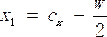 (2)
(2)
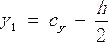 (3)
(3)
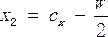 (4)
(4)
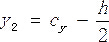 (5)
(5)
Where cx, cy is Normalized horizontal/vertical center coordinates of the predicted bounding box (scaled to the input image size of 640 x 480). w, h is the Normalized width/height of the predicted bounding box (scaled to the input image size). - Filter the YOLOv10’s output by the confidence threshold (0.5) to retain only EBike-related detections (class ID corresponding to electric bike), then process with NMS (IoU=0.45) to remove redundant boxes. Convert the remaining bounding box to [x1, y1, x2, y2] for ROI cropping.
- Handling multiple detections
NOTE: In elevator scenarios (the core target of the EBike-DET dataset), EBikes are typically single-instance (due to space constraints). For cases with multiple EBike detections (e.g., crowded elevators with two EBikes), the following rules apply.- Highest-confidence priority: Select the bounding box with the maximum confidence score (YOLOv10’s output confidence reflects the model’s certainty of the object being an EBike).
- Spatial validity check: If multiple detections have confidence scores >0.7, verify the spatial overlap with elevator structural boundaries (e.g., avoid bounding boxes extending beyond elevator walls). Retain the detection whose center point cx, cy, is closest to the image center (elevators are typically monitored by front-facing cameras, with targets centered).
- Edge case handling: If no valid detections meet the confidence threshold (e.g., severe occlusion), mark the image for manual ROI correction (accounting for <3% of the EBike-DET dataset).
- To ensure reproducibility of ROI localization, apply the inference parameters from Table 4 for YOLOv10 (using the yolov10x.pt pre-trained weight file). The output bounding box coordinates are as follows:
- Grayscale conversion and normalization
- Perform grayscale conversion on the cropped RGB image from the ROI. Use the weighted average method for conversion, following the formula:
Igra = 0.299 × R + 0.587 × G + 0.114 × B (6)
where R, G, and B represent the pixel values in the red, green, and blue channels, respectively. This method aligns with human perception of brightness across different colors. - Normalize the pixel values of the grayscale image to the range of [0, 1] by linearly scaling from [0, 255]. This normalization improves the stability of numerical calculations and ensures that subsequent gradient computations and thresholding work consistently under varying lighting conditions.
- Perform grayscale conversion on the cropped RGB image from the ROI. Use the weighted average method for conversion, following the formula:
- Harris corner detection
- Apply Harris corner detection to the grayscale and normalize EBike region to extract local feature points.
NOTE: The core principle of Harris corner detection involves computing the autocorrelation matrix to accurately locate the corners in the image, as visually shown in Figure 4B. These detected corners are typically associated with key EBike components such as wheels, front area, and rear area, which often exhibit clear corner features. - Compute the gradient of the image to identify areas of significant intensity changes as described below.
- Image smoothing: Apply Gaussian filtering to the grayscale image to suppress noise, obtaining the smoothed image as follows:
Is = Gσ*I (7)
where * represents the convolution operation, and Gσ is a 2D Gaussian kernel with a standard deviation of σ, which controls the smoothing level. A typical value for is 1.0. - Compute image gradient: Use a gradient operator (such as the Sobel operator) to calculate the horizontal (x) and vertical (y) gradients of the smoothed image:
Ix = Kx * Is ,Iy=Ky * Iy (8)
where Ix and Iy are the gradient maps in the x and y directions, respectively, and Gx and Gy are the convolution kernels for the Sobel operator:
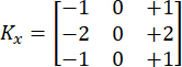 ,
, 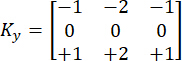 (9)
(9) - Construct autocorrelation matrix M based on the previously computed gradients, using a 3 x 3 local window W centered at each pixel (x,y):
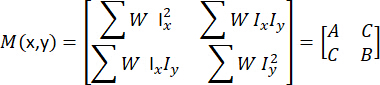 (10)
(10)
In the formula, W refers to a local window at position (x,y), and the operation ∑W represents the summation of all image elements within this window; A = ∑W Ix2 represents the sum of the squared gradients in the W window in the x direction, reflecting the intensity of changes in the x direction; B=∑W Iy2 represents the sum of the squared gradients in the W window in the y direction, reflecting the intensity of changes in the y direction; C = ∑W IxIy represents the sum of the product of the gradients in the x and y directions within the W window, describing the correlation of changes between these two directions. - Compute the sum of squared gradients in both the x and y directions to reflect the intensity of changes along each direction. The cross-term between the gradients Ix Iy captures the correlation between the x and y directions.
- Corner response function: Compute the corner response function R based on the determinant and trace of the autocorrelation matrix to detect corner points in the image. Calculate the response value for each pixel and select points with higher response values as the final corners as shown in Figure 2. The corner response function is given by:
det(M) = A ⋅ B - C2 (11)
trace(M) = A + B (12)
R = det(M) - k ⋅ (trace(M))2 (13)
where det(M) is the determinant of the M, reflecting the overall change in the local feature region, and trace(M) is the trace of the matrix, reflecting the total gradient intensity in the region. The empirical constant k is typically set between 0.04 and 0.06.
NOTE: Based on experiments, it was found that the choice of k significantly influences the results:
When k=0.04, the response values are too high, leading to an overabundance of falsely detected corner points.
When k=0.05, the response values are more balanced, accurately detecting true corners.
When k=0.06, the response values are too low, making it difficult to reliably detect corner points.
- Image smoothing: Apply Gaussian filtering to the grayscale image to suppress noise, obtaining the smoothed image as follows:
- Perform coarse-grained division of the local areas of the EBike using the Harris corner-point detection results. Divide the EBike into regions based on geometric structure and corner point distribution, as shown in Figure 4C, to improve the model’s robustness and detection performance in complex occlusion scenarios.
- Wheel area: Consider the region valid if it contains at least 15 corner points that are symmetrically distributed along a circular shape, with a symmetry score of no less than 0.85. The symmetry score is shown in Equation 11. The width-to-height ratio of the wheel region should be approximately 1:1, ensuring it accurately reflects the geometric characteristics of the wheel.
- Front area: Include the region if it contains at least 10 corner points with a symmetry score no less than 0.80, and the width-to-height ratio falls between 1.2:1 and 1.5:1, ensuring that the front area corresponds to the expected structural features.
- Rear area: Include the region if it contains at least 12 corner points, with a symmetry score no less than 0.75, and the width-to-height ratio range between 1.5:1 and 2:1, ensuring that the rear area adheres to the expected geometric properties.
- Apply Harris corner detection to the grayscale and normalize EBike region to extract local feature points.
- Representation of critical EBike areas with bounding boxes
- To convert corner points into rectangular bounding boxes, use the DBSCAN clustering algorithm. This method groups nearby corner points into clusters, ensuring that corner points forming a region are grouped together. Set the maximum distance between points within a cluster to 30 pixels.
- For each cluster of corner points, determine the minimum and maximum x and y coordinates. These coordinates represent the edges of the bounding box.
- Add a margin of 10 pixels around the bounding box to ensure all relevant features are included. This margin compensates for potential misalignment or pixel inaccuracies in corner point detection.
- Round the bounding box coordinates to the nearest integer to ensure proper pixel alignment for image processing.
- Represent the final bounding box coordinates for the i-th component (e.g., wheel, front area, rear area) as described below.
- Combine the defined regions (wheel area, front area, and rear area) and represent all critical areas of the EBike using rectangular bounding boxes.
- Define bounding box coordinates for the i component (e.g., wheel, front area, rear area) as:
![Equation of box coordinates, \( B_i = [x_1^i, y_1^i, x_2^i, y_2^i] \), in mathematical notation.](/files/ftp_upload/69226/69226eq208.jpg "figure-protocol-8") (14)
(14)
where Bi represents the bounding box of the i-th component, and and are the coordinates of the upper-left and lower-right corners, respectively.
- Handling partial occlusion
- Evaluate the corner-symmetry score for each region. Accept a region if the symmetry score is greater than or equal to 0.7.
- For occlusion handling, measure the visibility of corner points. Accept a region if at least 50% of the corners are visible. If 30%-50% of the corners are visible, flag the region for further review. If less than 30% of the corners are visible, reject the region due to insufficient visibility for accurate detection.
- Accuracy judgment of local feature regions
- Evaluate the accuracy of each local feature region using three quantitative operational metrics: a symmetry metric S, a contour continuity metric C, and a connection-structure metric L. Apply these metrics uniformly to the wheel area, front area, and rear area.
- Accept a region only when all metrics meet the predefined thresholds. If one metric fails within a tolerable range, expand the ROI and re-evaluate. If two or more metrics fail, mark the region as unreliable.
- Wheel-region feature accuracy analysis
- Front view operational checkpoint
- Compute the symmetry metric:
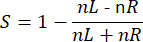 (15)
(15)
where nL and nR denote the left- and right-side corner counts. - Accept the region if S ≥ 0.85. As shown in Figure 5A, the wheel exhibits a circular shape with symmetry, and Harris corner points along the circumference form a symmetrical pattern. So, annotate the entire wheel area.
- If 0.70 ≤ S<0.85, expand the ROl by 10-20 pixels and repeat the evaluation to allow more real features to re-enter the computation area, and then re-evaluate. As shown in Figure 5D, partial occlusion of the wheel occurs, so the cropping range should be expanded to capture more features of the Ebike for evaluation.
- If S<0.70, label the region as unreliable. As shown in Figure 5G, the circular shape is disrupted; exclude this region from annotation.
- Compute the symmetry metric:
- Side view operational checkpoint
- Measure contour continuity using:
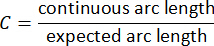 (16)
(16) - Accept when C ≥ 0.75. As shown in Figure 5B, the ratio of the actual continuous arc length to the expected arc length meets the requirements, the contour fully fits the edge, and there is no obvious breakage.
- If 0.55 ≤ C < 0.75, refine the contour extraction and re-check. As shown in Figure 5E, the current ratio of the continuous arc length to the expected arc length is in the critical range; it is necessary to adjust the threshold of the extraction algorithm to make the contour more complete.
- If C < 0.55, reject the region due to insufficient geometric continuity. As shown in Figure 5H, the analysis requirements cannot be met.
- Measure contour continuity using:
- Top view operational checkpoint
- Evaluate structural connectivity using:
 (17)
(17) - Accept when L ≥ 0.70. As shown in Figure 5C, the deviation between the observed distance and the expected distance is effectively offset, the structural connectivity meets the requirements, and the relative position connection between the vehicle and the elevator environment is complete.
- If L < 0.70, expand the ROI and re-evaluate. As shown in Figure 5F, the current deviation between the observed distance and the expected distance is relatively large; it is necessary to expand the analysis scope and include more surrounding structures to improve the accuracy of connectivity evaluation.
- If connectivity remains inconsistent, classify the region as unreliable. As shown in Figure 5I, it cannot be used as an effective analysis area.
- Evaluate structural connectivity using:
- Front view operational checkpoint
- Front area feature accuracy analysis
- For the feature accuracy evaluation of the EBike front area, follow the unified rule-based framework defined in Section 2.10, including symmetry evaluation under the front view using metric S as defined in Equation 15, contour continuity assessment under the side view using metric C as defined in Equation 16, and structural connectivity validation under the top view using metric L as defined in Equation 17.
- Due to geometric variability and frequent partial occlusion in the front area, adopt a moderately relaxed thresholds compared with the wheel region. A front-area region is accepted when S ≥ 0.80, C ≥ 0.70, and L ≥ 0.65. As illustrated in Figure 6A-C, regions satisfying these criteria exhibit balanced left–right feature distributions, coherent contours, and stable structural connectivity.
- If any metric falls within the intermediate range specified in Section 2.10, expand the region of interest and re-evaluate to incorporate additional contextual features, as shown in Figure 6D-F. Regions that fail to meet the minimum criteria after re-evaluation, classify as unreliable, as illustrated in Figure 6G-I.
- Rear-Area Feature Accuracy Analysis
- For the rear-area feature accuracy analysis, adhere to the evaluation protocol defined in Section 2.10, employing metrics S as defined in Equation 15, C as defined in Equation 16, and L as defined in Equation 17 under front, side, and top views, respectively.
- The rear area is more susceptible to occlusion caused by riders, carried objects, or elevator structures. Therefore, apply stricter rejection conditions to avoid unreliable annotations. A rear-area region is accepted when S ≥ 0.75, C ≥ 0.70, and L ≥ 0.65. Representative accepted cases with sufficient symmetry, contour continuity, and connectivity are shown in Figure 7A-C.
- For regions with borderline metric values, perform ROI expansion and re-evaluation, as illustrated in Figure 7D-F. If the geometric relationships remain ambiguous or the metrics fail to satisfy the acceptance criteria, mark the region as unreliable, as shown in Figure 7G-I.
- Rear Area Feature Accuracy Analysis
- For the rear area feature accuracy analysis, follow the evaluation protocol defined in Section 2.10, using the same metrics S as defined in Equation 15, C as defined in Equation 16, and L as defined in Equation 17 under corresponding viewpoints.
- Compared with the front area, the rear area is more susceptible to occlusion caused by riders, carried objects, and elevator interior structures. Therefore, apply slightly stricter rejection criteria to prevent unreliable annotations. A rear-area region is accepted when S ≥ 0.75, C ≥ 0.70, and L ≥ 0.65. As shown in Figure 7A-C, accepted regions maintain sufficient symmetry, contour coherence, and structural connectivity.
- For regions with borderline metric values, expand and re-evaluate the ROI following Section 2.10, as illustrated in Figure 7D-F. If the geometric consistency remains insufficient after re-evaluation, mark the region as unreliable, as shown in Figure 7G-I.
- Implementation of the pipeline
- File and folder structure: The implementation follows a modular directory structure separating detection, local feature extraction, and annotation judgment. See the representative folder organization shown below. Store all intermediate results in dedicated subfolders to allow independent inspection of each processing step.
project_root/
│
├── data/
│ ├── images/
│ │ ├── train/
│ │ ├── val/
│ │ └── test/
│ └── annotations/
│
├── detection/
│ ├── detect_ebike.py
│ └── yolov10_config.yaml
│
├── roi/
│ ├── crop_roi.py
│ └── cropped_images/
│
├── harris/
│ ├── harris_corner.py
│ └── corner_visualization/
│
├── chunk_annotation/
│ ├── region_partition.py
│ ├── validity_judgment.py
│ └── final_annotations/
│
└── configs/
└── thresholds.yaml - Execution pipeline and example command lines
- EBike detection and ROI localization: Localize EBike regions using a pre-trained object detection model. Store detection results as bounding box coordinates.
python detection/detect_ebike.py \
--input data/images/test/ \
--output roi/detections.json - ROI cropping: Use the detected bounding boxes to crop EBike regions from the original images.
python roi/crop_roi.py \
--detections roi/detections.json \
--images data/images/test/ \
--output roi/cropped_images/
Save each cropped image using the naming format: imageID_roi_xmin_ymin_xmax_ymax.jpg - Harris corner extraction: Apply Harris corner detection to each cropped ROI after grayscale conversion. Save corner response maps and visual overlays for inspection.
python harris/harris_corner.py \
--input roi/cropped_images/ \
--output harris/corner_visualization/ \
--config configs/thresholds.yaml - Coarse-grained partitioning and chunk annotation: Partition local feature regions into wheel, front area, and rear area based on the spatial distribution of corner points. Apply validity judgment using geometric and feature-based criteria.
python chunk_annotation/region_partition.py \
--corners harris/corner_visualization/ \
--output chunk_annotation/final_annotations/
- EBike detection and ROI localization: Localize EBike regions using a pre-trained object detection model. Store detection results as bounding box coordinates.
- Expected intermediate outputs and visual checkpoints: Save the intermediate outputs produced by each processing stage that serve as visual checkpoints.These intermediate outputs enable step-by-step verification of ROI localization, corner extraction quality, region partitioning, and final annotation decisions.
- ROI cropping output: Save cropped EBike images in roi/cropped_images/. Each image contains a single EBike region extracted from the original frame.
- Harris corner visualization: Save corner overlays in harris/corner_visualization/. For valid wheel regions, a dense set of corner points is observable along the circular rim structure. Regions with insufficient corner responses are identifiable at this stage.
- Region partitioning results: Visualize partitioned regions (wheel, front area, rear area) independently. Only retain regions that satisfy predefined validity criteria (e.g., sufficient corner density and geometric consistency).
- Final annotation output: Store accepted regions in chunk_annotation/final_annotations/ as structured annotation files. Exclude regions failing validity judgment and do not propagate them to subsequent stages.
NOTE: All thresholds used for corner detection and region validity judgment are centralized in configuration files. The pipeline operates on single-frame inputs without temporal dependency, allowing results to be reproduced independently for each image. Given identical input images, configuration files, and execution order, the generated intermediate outputs and final annotations remain deterministic.
- File and folder structure: The implementation follows a modular directory structure separating detection, local feature extraction, and annotation judgment. See the representative folder organization shown below. Store all intermediate results in dedicated subfolders to allow independent inspection of each processing step.
- Finalization steps and dataset release
NOTE: To ensure that the protocol terminates with a clear and reproducible endpoint, a finalization stage is defined to consolidate annotation saving, quality validation, dataset packaging, and version documentation.- Saving final annotations: After region validity judgment, save all accepted annotations in chunk_annotation/final_annotations/ using the YOLO text format, with one annotation file corresponding to each image. Retain only regions that satisfy the predefined geometric and feature-based criteria in the final annotation set and exclude rejected or unreliable regions from further use.
- Annotation quality validation: Validate final annotation quality by reapplying the same validity criteria used during region evaluation, including symmetry, contour continuity, and structural connectivity metrics. Remove annotations that fail to meet these criteria during this verification stage, ensuring consistency between annotation generation and quality control.
- Dataset packaging: Following validation, organize images and annotations into fixed training, validation, and test splits according to the defined dataset partition. The directory structure and file lists are frozen at this stage, and the packaged dataset is prepared for training and evaluation without further modification.
- Version and seed documentation: Configuration files, including corner detection parameters and region validity thresholds, are preserved together with the packaged dataset. Use random seeds for data splitting, fix algorithm execution, and record. In addition, document the versions of model weights, configuration files, and annotation tools. Given identical input data, configuration files, and recorded seeds, the final annotations and dataset splits remain deterministic.
3. Data augmentation
NOTE: A previous study has shown that training datasets lacking sufficient preprocessing and data augmentation often result in degraded model performance22. To address these challenges, the following procedure was followed.
- Lighting
- Simulate lighting variations inside elevators to address frequent illumination changes by adjusting the brightness factor within the range of 0.6–1.4, with a probability of 0.8.
- Apply light intensity adjustments to transition from bright to dim environments, simulating EBike movement-induced blurring. Use a probability of 0.7 for this operation.
- Generate augmented samples by adjusting lighting conditions, ensuring stable visibility under varying illumination levels.
- Apply these lighting operations offline and store them for subsequent processing. Set the random seed to 42 to ensure reproducibility of the augmentation process.
- Occlusion
- Create synthetic occlusion scenarios to reflect crowded elevator conditions. Apply occlusion masks (e.g., human silhouettes, object blocks) with a probability of 0.6.
- Apply mosaic occlusions to mimic partial obstruction of EBikes during elevator entry and exit. Use occlusion percentages of 30%, 50%, or 70%, and ensure the occlusion is applied randomly in any quadrant (top, bottom, left, right) of the image.
- Incorporate occluded samples to improve detection robustness and stability under partial visibility, ensuring at least one key component (e.g., wheel, front area, rear area) remains visible.
- Perform occlusion augmentation offline and validate the samples to ensure that essential EBike features are retained. Set the random seed to 42 for reproducibility.
- Viewpoints
- Adjust viewing angles within a predefined range of ±15° to simulate diverse camera angles in different elevator environments. This operation should be applied with a probability of 0.7.
- Apply perspective transformations with distortion coefficients between 0.0 and 0.2 to replicate different camera placements (e.g., elevated, side, and oblique viewpoints).
- Scale and shift the EBike region by 0.8–1.2 times to simulate changes in the camera’s distance from the target. Apply this transformation with a probability of 0.8.
- Confirm that all viewpoint transformations retain the EBike’s geometric integrity and that no critical features are distorted.
- Perform viewpoint transformations offline and store the augmented images. Set the random seed to 42 for reproducibility.
- Enhancement
- Apply grayscaling to 30% of the images with a probability of 0.3 to introduce luminance-driven variations and enhance model robustness under low-light conditions.
- Use histogram equalization on 20% of the samples to enhance contrast and visibility of the EBike’s key features under challenging lighting conditions.
- Combine lighting, occlusion, and viewpoint augmentation strategies sequentially to generate high-diversity samples. Use probabilities of 0.9 for this multi-step process.
- Review the augmented samples to ensure they maintain EBike structural integrity before integrating them into the final dataset.
- Perform enhancement operations offline and store the images for subsequent training use. Set the random seed to 42 to ensure reproducibility of the entire augmentation process.
4. Experimental environment
- Configure the experimental environment to ensure computational efficiency and stability during model training and testing.
- Use a modern multi-core processor, a dedicated GPU for deep-learning acceleration, sufficient memory, and a stable storage system to support large-scale EBike image data processing.
- Match the software environment with the hardware configuration by installing compatible versions of the deep-learning framework, GPU drivers, and acceleration libraries to optimize training speed and inference performance.
- Refer to Table 5, Table 6, Table 7, and Table 8 for detailed hardware specifications, software environment, model dependencies, and imaging equipment settings to ensure reproducibility.
- Computational overhead and runtime analysis
- Analyze the computational overhead associated with the chunked annotation strategy in terms of annotation complexity and runtime efficiency. Compared with holistic annotation, chunked annotation represents an EBike using part-level regions, including the wheel area, front area, and rear area. Annotate these regions only when they are visible and satisfy the predefined geometric and feature-based validity criteria, rather than being enforced for every instance.
NOTE: From the annotation perspective, the increase in label count remains limited and structurally constrained. An EBike instance contributes at most three part-level annotations, while fewer regions are annotated in cases of partial occlusion (e.g., when only the front area is visible). As a result, the number of labels per image varies with scene visibility and occlusion conditions, and the average label count increases moderately, as summarized in Table 9. This design balances local feature representation with annotation complexity. From the inference perspective, chunked annotation does not introduce a proportional increase in post-processing cost. Although part-level detection may generate additional candidate bounding boxes, detections are aggregated at the EBike object level for final evaluation, and confidence-based filtering is applied prior to post-processing. This conditional, visibility-driven annotation strategy limits unnecessary detection candidates. For models such as YOLOv10, which reduce reliance on traditional non-maximum suppression, the additional overhead introduced by chunking remains limited in practice. - Evaluate runtime performance at a typical elevator surveillance resolution of 640 x 480 pixels using an NVIDIA RTX 3090 GPU. As shown in Table 9, chunked annotation maintains real-time inference capability, with only a minor reduction in frames per second compared with holistic annotation. These results indicate that the chunked annotation strategy remains suitable for real-time EBike monitoring in elevator environments.
- Analyze the computational overhead associated with the chunked annotation strategy in terms of annotation complexity and runtime efficiency. Compared with holistic annotation, chunked annotation represents an EBike using part-level regions, including the wheel area, front area, and rear area. Annotate these regions only when they are visible and satisfy the predefined geometric and feature-based validity criteria, rather than being enforced for every instance.
5. Evaluation metrics
NOTE: Although chunked annotations are used during training and inference, evaluation is performed at the e-bike object level. Part-level detections are aggregated into a single e-bike decision according to the rules defined in Section 2.4,3.
- Apply standard evaluation metrics commonly used in target-detection research27 to comprehensively assess algorithm performance in EBike occlusion-detection scenarios.
- Detection precision (P)
- Use Equation (8) to compute detection precision, which measures the proportion of correctly identified EBikes among all predicted positive samples.
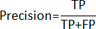 (18)
(18)
where TP denotes true positives and FP denotes false positives. - Set the IoU threshold to 0.5 to determine whether the predicted bounding boxes match the ground-truth boxes.
- Use precision to assess the model’s capability to reduce unnecessary alarms caused by misidentification of non-EBike objects.
- Command(s) to generate this metric: Use the relevant evaluation script (e.g., evaluate_precision.py). Save results in precision_results.txt for further analysis.
- Use Equation (8) to compute detection precision, which measures the proportion of correctly identified EBikes among all predicted positive samples.
- Recall rate (R)
- Use Equation (9) to determine how effectively the model identifies EBikes in elevator environments, particularly when occlusion affects visibility.
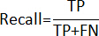 (19)
(19)
where FN represents false negatives. - Set the IoU threshold at 0.5 to assess the accuracy of detections. Use recall to evaluate the model’s ability to minimize missed detections, ensuring that EBikes remain accurately identified even when partially obstructed.
- Use command(s) to generate this metric: run evaluate_recall.py. Save results in recall_results.txt.
NOTE: Missed detections are critical in crowded elevator scenarios and must be minimized for safety. Missed detections pose safety concerns in crowded elevator scenarios and must be minimized.
- Use Equation (9) to determine how effectively the model identifies EBikes in elevator environments, particularly when occlusion affects visibility.
- F1-score
- Calculate the F1-score using Equation (10) to obtain a balanced representation of the model’s precision and recall performance.
 (20)
(20) - Use the F1-score to provide a holistic assessment, especially in scenarios where precision and recall exhibit trade-offs under varying occlusion levels.
- Use Command(s) to generate this metric: Run evaluate_f1.py to compute the F1-score. Save results in f1_score_results.txt.
- Calculate the F1-score using Equation (10) to obtain a balanced representation of the model’s precision and recall performance.
- Mean average precision (mAP)
- Use Equation (11) to measure the overall detection capability of the model across varying EBike appearances, occlusion conditions, and lighting variations.
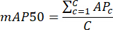 (21)
(21)
Where APc denotes the average precision of category c and C is the number of categories. - Set IoU threshold to 0.5 to evaluate the model’s performance across different categories.
- Use mAP@0.5 to determine how well the model adapts to diverse visual conditions in elevator settings, ensuring comprehensive evaluation of detection performance.
- Use the following command(s) to generate this metric: execute evaluate_map.py with the specified parameters. Save results in map_results.txt.
- Use Equation (11) to measure the overall detection capability of the model across varying EBike appearances, occlusion conditions, and lighting variations.
Access restricted. Please log in or start a trial to view this content.
Results
Comparison of holistic annotation and chunked annotation on public dataset
The evaluation was conducted on a public dataset comprising 210 EBike images collected from open surveillance and traffic monitoring scenes, with diverse lighting conditions, EBike colors, and varying degrees of occlusion. Each image was annotated using both the holistic method (single bounding box) and the proposed chunked method (dividing EBikes into wheels, front area, and rear areas).
Access restricted. Please log in or start a trial to view this content.
Discussion
Critical steps
A critical step in this protocol is the chunked annotation method based on local features, where EBikes are segmented into wheel, front, and rear areas. This division ensures that detection models can learn fine-grained representations, which proved essential in occlusion-heavy elevator environments. For instance, YOLOv5 trained with chunked annotations on the EBike-DET dataset improved its mAP@0.5 from 0.925 to 0.966, underscoring the necessity of accurate loc...
Access restricted. Please log in or start a trial to view this content.
Disclosures
The authors have no conflicts of interest.
Acknowledgements
This work was supported by the 2025 Humanities and Social Sciences Research Planning Fund of the Ministry of Education of China (Grant No.25YJAZH002), the 2024 Guangdong Province Key Discipline Research Capacity Enhancement Project (Grant No.2024ZDJS086), the Guangdong Provincial Undergraduate Innovation and Entrepreneurship Training Program in 2024 (Grant No.S202413714017), and The Ministry of Education's Employment-Education Connection Program: "Innovation and Practice of Talent Cultivation Mechanism for Computer Application Majors Oriented to Artificial Intelligence Technology" (Grant No. 2025072869464).
Access restricted. Please log in or start a trial to view this content.
Materials
| Name | Company | Catalog Number | Comments |
|---|---|---|---|
| h5py (SSD) | HDF Group | 2.10.0 | |
| matplotlib (SSD) | Matplotlib Community | 3.1.2 | |
| matplotlib (YOLOv10) | Matplotlib Community | 3.9.0 | |
| matplotlib (YOLOv5) | Matplotlib Community | 3.8.4 | |
| matplotlib (YOLOv5+SAHI) | Matplotlib Community | 3.8.4 | |
| matplotlib (YOLOv8-Seg) | Matplotlib Community | 3.9.0 | |
| numpy (SSD) | NumPy Community | 1.17.0 | |
| numpy (YOLOv10) | NumPy Community | 1.26.3 | |
| numpy (YOLOv5) | NumPy Community | 1.26.4 | |
| numpy (YOLOv5+SAHI) | NumPy Community | 1.26.4 | |
| numpy (YOLOv8-Seg) | NumPy Community | 1.26.3 | |
| onnx (YOLOv10) | ONNX | 1.14.0 | |
| onnx (YOLOv5) | ONNX | 1.14.0 | |
| onnx (YOLOv5+SAHI) | ONNX | 1.14.0 | |
| onnxruntime (YOLOv10) | Microsoft | 1.15.1 | |
| onnxruntime (YOLOv5) | Microsoft | 1.15.1 | |
| onnxruntime (YOLOv5+SAHI) | Microsoft | 1.15.1 | |
| opencv-python (SSD) | OpenCV | 4.1.2.30 | |
| opencv-python (YOLOv10) | OpenCV | 4.9.0.80 | |
| opencv-python (YOLOv5) | OpenCV | 4.9.0.80 | |
| opencv-python (YOLOv5+SAHI) | OpenCV | 4.9.0.80 | |
| opencv-python (YOLOv8-Seg) | OpenCV | 4.9.0.80 | |
| pandas (YOLOv10) | Pandas Community | 2.2.2 | |
| pandas (YOLOv5) | Pandas Community | 2.2.2 | |
| pandas (YOLOv5+SAHI) | Pandas Community | 2.2.2 | |
| pandas (YOLOv8-Seg) | Pandas Community | 2.2.2 | |
| Pillow (SSD) | Pillow Developers | 8.2.0 | |
| Pillow (YOLOv10) | Pillow Developers | 10.2.0 | |
| Pillow (YOLOv5) | Pillow Developers | 8.5.0 | |
| Pillow (YOLOv5+SAHI) | Pillow Developers | 8.5.0 | |
| Pillow (YOLOv8-Seg) | Pillow Developers | 10.2.0 | |
| psutil (YOLOv10) | Psutil Developers | 5.9.8 | |
| psutil (YOLOv5) | Psutil Developers | 5.9.8 | |
| psutil (YOLOv5+SAHI) | Psutil Developers | 5.9.8 | |
| pycocotools (YOLOv10) | COCO Consortium | 2.0.7 | |
| pycocotools (YOLOv5) | COCO Consortium | 2.0.7 | |
| pycocotools (YOLOv5+SAHI) | COCO Consortium | 2.0.7 | |
| pycocotools (YOLOv8-Seg) | COCO Consortium | 2.0.7 | |
| py-cpuinfo (YOLOv10) | Py-CPUInfo Developers | 9.0.0 | |
| py-cpuinfo (YOLOv5) | Py-CPUInfo Developers | 9.0.0 | |
| py-cpuinfo (YOLOv5+SAHI) | Py-CPUInfo Developers | 9.0.0 | |
| PyYAML (YOLOv10) | PyYAML | 6.0.1 | |
| PyYAML (YOLOv5) | PyYAML | 6.0.1 | |
| PyYAML (YOLOv5+SAHI) | PyYAML | 6.0.1 | |
| PyYAML (YOLOv8-Seg) | PyYAML | 6.0.1 | |
| requests (SSD) | Python Requests | 2.27.1 | |
| requests (YOLOv10) | Python Requests | 2.32.3 | |
| requests (YOLOv5) | Python Requests | 2.31.0 | |
| requests (YOLOv5+SAHI) | Python Requests | 2.31.0 | |
| SAHI | SAHI Developers | 0.3.4+ | |
| scipy (SSD) | SciPy Community | 1.2.1 | |
| scipy (YOLOv10) | SciPy Community | 1.13.0 | |
| scipy (YOLOv5) | SciPy Community | 1.13.0 | |
| scipy (YOLOv5+SAHI) | SciPy Community | 1.13.0 | |
| scipy (YOLOv8-Seg) | SciPy Community | 1.13.0 | |
| seaborn (YOLOv10) | Seaborn Developers | 0.13.2 | |
| seaborn (YOLOv5) | Seaborn Developers | 0.13.2 | |
| seaborn (YOLOv5+SAHI) | Seaborn Developers | 0.13.2 | |
| seaborn (YOLOv8-Seg) | Seaborn Developers | 0.13.2 | |
| shapely (YOLOv5+SAHI) | Shapely Developers | 2.0.4 | |
| SSD | Caffe/Original SSD Authors | Python 3.6.13+; PyTorch 1.2.0+; CUDA 10.0; CUDNN 7.4.1 | |
| tensorboard (SSD) | 2.10.1 | ||
| tensorboard (YOLOv5) | 2.16.2 | ||
| tensorboard (YOLOv5+SAHI) | 2.16.2 | ||
| torchvision (SSD) | PyTorch | 0.4.0 | |
| torchvision (YOLOv10) | PyTorch | 0.15.2 | |
| torchvision (YOLOv5) | PyTorch | 0.17.2 | |
| torchvision (YOLOv5+SAHI) | PyTorch | 0.17.2 | |
| torchvision (YOLOv8-Seg) | PyTorch | 0.16.1+ | |
| tqdm (SSD) | TQDM Developers | 4.60.0 | |
| tqdm (YOLOv10) | TQDM Developers | 4.66.4 | |
| tqdm (YOLOv5) | TQDM Developers | 4.66.2 | |
| tqdm (YOLOv5+SAHI) | TQDM Developers | 4.66.2 | |
| ultralytics (YOLOv8-Seg) | Ultralytics | 8.2.99+ | |
| YOLOv10 | YOLOv10 Team | Python 3.8.0+; PyTorch 2.0.1+cu118; CUDA 11.8; CUDNN 8.7 | |
| YOLOv5 | Ultralytics | Python 3.8.0+; PyTorch 2.2.2+; CUDA 11.2; CUDNN 8.1.2 | |
| YOLOv5 + SAHI | Ultralytics + SAHI Developers | Python 3.8.0+; PyTorch 2.2.2+; CUDA 11.2; CUDNN 8.1.2 | |
| YOLOv8-Seg | Ultralytics | Python 3.8.0+; PyTorch 2.0.1+cu118; CUDA 11.8; CUDNN 8.6.0+ |
References
- Li, Y., Han, L., Ning, X., Xu, Y. Fire risk of electric bicycle based on fuzzy Bayesian network. J Phys Conf Ser. 1578 (1), 012153-012160 (2020).
- Cao, F., Sheng, G., Feng, Y. Detection dataset of electric bicycles for lift control. Alexandria Eng J. 105 (1), 736-742 (2024).
- Zhang, J., Mohd Yunos, Z., Haron, H. Interactivity recognition graph neural network model for improving human-object interaction detection. Electronics. 12 (2), 470-482 (2023).
- Yang, D., Su, C., Wu, H., Xu, X., Zhao, X. Shelter identification for shelter-transporting AGV based on improved YOLOv5. IEEE Access. 10 (1), 119132-119139 (2022).
- Wang, X., et al. LDS-YOLO: A lightweight small object detection method for dead trees. Comp Electron Agri. 198 (1), 107035-107044 (2022).
- Xu, R., Zhu, D., Chen, M. A novel underwater object detection enhanced algorithm based on YOLOv5-MH. IET Image Process. 18 (10), 3415-3429 (2024).
- Shang, J., Wang, J., Liu, S., Wang, C., Zheng, B. Small target detection algorithm for UAV aerial photography based on improved YOLOv5s. Electronics. 12 (11), 2434-2446 (2023).
- Wang, C. Y., Liao, H. Y. M. YOLOv1 to YOLOv10: The fastest and most accurate real-time object detection systems. APSIPA Trans Signal Inf Process. 13 (1), 1-18 (2024).
- Sapkota, R., et al. YOLO11 to its genesis: A decadal and comprehensive review of the YOLO series. Artif Intell Rev. 58 (2), 145-182 (2025).
- Huang, Z., Yin, Z., Ma, Y., Fan, C., Chai, A. Mobile phone component object detection based on improved SSD. Procedia Comp Sci. 183 (1), 107-114 (2021).
- Li, Y., Yang, F., Li, Y., Tan, C., Liu, Z. Circuit breaker identification based on SSD. J Phys Conf Ser. 2418 (1), 012080-012088 (2023).
- Deng, X., Li, S. Improved SSD object detection based on attention mechanism and feature fusion. J Phys Conf Ser. 2450 (1), 012088-012096 (2023).
- Huo, B., Li, C., Zhang, J., Xue, Y., Lin, Z. SAFF-SSD: Self-attention combined feature fusion SSD for small object detection. Remote Sens. 15 (12), 3027-3041 (2023).
- Murphy, K., Torralba, A., Eaton, D., Freeman, W. Object detection and localization using local and global features. Lect Notes Comp Sci. 4170 (1), 382-400 (2006).
- Mamat, N., Othman, M. F., Abdulghafor, R., Alwan, A. A., Gulzar, Y. Enhancing image annotation technique for fruit classification using deep learning. Sustainability. 15 (2), 901-915 (2023).
- Zhang, T., Jia, K., Xu, C., Ma, Y., Ahuja, N. Partial occlusion handling via robust part matching. Proc IEEE CVPR. 2014 (1), 1258-1265 (2014).
- Howard, A. G. Improvements on deep convolutional neural network based image classification. Tech Rep. 1 (1), 1-12 (2013).
- Zhang, H. Mixup: Beyond empirical risk minimization. arXiv. , (2017).
- Krizhevsky, A., Sutskever, I., Hinton, G. E. ImageNet classification with deep convolutional neural networks. Commun ACM. 60 (6), 84-90 (2017).
- Qin, J., Xu, N. Social distancing monitoring based on SSD. Procedia Comp Sci. 183 (1), 768-775 (2021).
- Zhong, P., Liu, Y., Zheng, H., Zhao, J. Detection of urban flood inundation using traffic images. Water Resour Manag. 38 (2), 287-301 (2024).
- Aamir, S. M., Ma, H., Khan, M. A. A., Aaqib, M. Real-time object detection in occluded environments with background clutter. Multimed Tools Appl. 83 (4), 11245-11261 (2024).
- Jia, K., Niu, Q., Wang, L., Niu, Y., Ma, W. Multi-object detection and size calculation for blended tobacco shreds. Sensors. 23 (18), 8380-8395 (2023).
- Sun, S., et al. Multi-YOLOv8 for infrared moving small object detection. Neurocomputing. 588 (1), 127685-127696 (2024).
- Sadik, M. N., Hossain, T., Sayeed, F. Real-time detection and analysis of vehicles and pedestrians using deep learning. Int J Comp Vis Robot. 14 (3), 215-229 (2024).
- Zhang, C., Jiao, P. YOLO series target detection algorithms for underwater environments. Ocean Eng. 279 (1), 114353-114366 (2023).
- Luo, B., Xiong, J., Xu, L., Pei, Z. Superpixel segmentation based on global similarity and contour region transform. IEICE Transac Info Sys. E103D (3), 716-719 (2020).
- Hosain, M. T., Jim, J. R., Mridha, M. F., Kabir, M. M. Explainable AI approaches in deep learning: Advancements, applications and challenges. Comp Electr Eng. 117 (1), 109246-109268 (2024).
- Khurshid, S., Basharat, S., Afzal, S. The magic of artificial intelligence-2. Artif Intell Hum Health Dis. 1 (1), 29-46 (2025).
- Pan, W., Chen, J., Lv, B., Peng, L. Improved YOLOv9s-UI for underwater object detection. Appl Sci. 14 (14), 7162-7175 (2024).
- Zhang, J., Yunos, Z. M., Haron, H. Parallel multi-head graph attention network for human-object interaction detection. IEEE Access. 11 (1), 131708-131725 (2023).
- Li, L., Gao, S., Wu, F., An, X. MBAN: Multi-branch attention network for small object detection. PeerJ Comp Sci. 10 (1), e1965-e1980 (2024).
Access restricted. Please log in or start a trial to view this content.
Reprints and Permissions
This article has been published
Video Coming Soon