Modeling a Novel Self-Optimized Wolf Optimizer for a Heterogeneous Network Model for Energy and Node Lifetime Analysis

Summary

The research presents a protocol to implement and evaluate a self-optimized wolf optimizer (SOWO) for energy-aware clustering and routing in wireless sensor networks, with step-by-step settings and reproducible evaluation to improve lifetime, throughput, and residual energy.

Abstract

The vital services of surveillance, information collection, and data transmission from high-risk environments to safer locations are still provided by Wireless Sensor Networks (WSNs). These services are improved by the majority of energy-efficient routing protocols structured for this purpose. A homogeneous routing protocol is applied to decrease the energy utilization of far-off hubs more efficiently; however, the energy utilization rate is higher for this protocol, poorer dependability, and more unfavorable information broadcast to the Wireless Router (WR) or base station (BS) when employed for a longer timeframe. To overcome these drawbacks, a modified Self-Optimized Wolf Optimizer (SOWO) is employed in this research. Incorporating heterogeneous nodes into the current approach, selecting the head based on remaining energy introduces a multi-level interaction strategy throughout the connections. Employing an energy hole elimination method is the foundation of the developed routing technique. Each approach aims to extend the network's lifetime and reduce energy consumption. Based on the findings, the proposed routing scheme demonstrates superior consistency periods, residual energy, throughputs, and network lifespan compared to existing ones. The research addresses the classical clustered-WSN problem of maximizing lifetime and sustained delivery under tight per-node energy budgets while keeping load/fairness balanced. The simulation results show a 3.4% and 32.22% improvement in network stability and residual energy, respectively, over existing algorithms.

Introduction

Wireless Sensor Networks (WSN) and the Internet of Things (IoT) are widely applied to various technological issues¹. WSNs have been used in different conditions to help move items, such as robots executing different errands. From the origin, IoT has given basic help, particularly in collecting data from insecure fields². There are specific reasons why these techniques are currently being utilized in different systems³, for example, in horticulture, medical services, ecological observing, military investigation, structural management, traffic management, monitoring changes in the water level variation, and so on⁴.

In a wireless network environment, data are typically gathered and broadcast to a receiver node known as the base station (BS) for further processing⁵. The sensor nodes continually enhance the network's performance by efficiently using their limited resources. Concerning the works⁶, developing mechanisms to reduce node energy depletion and improve network lifetime can enhance wireless sensor network performance⁷. The different units of sensor nodes are used for higher energy: communication units, data processing units, and sensors. The first communication unit is the most energy-consuming⁸. In the environment of wireless sensor networks, the maximum energy-efficient techniques are regarded as hierarchical routing protocols widely used⁹. As the data are received from the neighbouring nodes, the Cluster Head (CH) uses single-hop and multi-hop interactions to report the network condition to the BS based on their remoteness from the BS. These types of routing techniques are given in the research¹⁰.

Several cluster-based routing algorithms for WSNs are anticipated in the related literature. A hierarchical routing scheme was proposed in Moridi et al.¹¹, which consecutively increases the lifespan of the supporting network. The considered network is selected appropriately based on the examination study¹², which developed a routing technique for network selection.

Priyadharshini et al.¹³ describe the probability-based clustering protocol known as distributed energy efficient clustering (DEEC). The CH chosen by DEEC depends on the ratio of the remaining energy to the mean energy of each node in the developed network. The authors investigated a homogeneous system known as the low-energy adaptive cluster hierarchy (LEACH) protocol and examined its heterogeneity. The authors then developed the LEACH, a heterogeneous system that compares two systems, homogeneous and heterogeneous¹⁴. A method developed by the distributed energy-effective clustering technique is proposed for heterogeneous remote sensor networks¹⁵. It is the upgraded variant of Distributed Energy-Effective clustering.

The experts proposed another advancement technique¹⁶. The novel algorithm changed the average likelihood of superior hubs whose remaining energy is not precisely the threshold residual energy value, which depends upon the typical space between the hubs and the BS instead of the usual network energy.

Distributed Energy-Effective clustering¹⁷ increased the possibility of the protocol's election by considering the average space among the SNs and the WR, as well as the distance between super nodes, when selecting cluster heads. The better E-DEEC efficiency in terms of throughputs, system lifetime, and surplus energy is depicted through the simulation outcomes. Nurelmadina et al.'s work is the critical element that encourages researchers to concentrate on this work¹⁸. Wireless sensor networks (WSNs) demand careful node placement because random deployment produces blind spots and broken links; maximizing coverage and preserving connectivity together is therefore a core optimization target rather than a nice-to-have. Prior art shows that classical swarm approaches (e.g., PSO/ACO) and ad-hoc deployment strategies often suffer from slow convergence and local-optima traps, which in turn yield low coverage and fragile connectivity¹⁹. A recent metaheuristic review highlights that such shortcomings typically stem from an imbalanced exploration-exploitation dynamic; it argues for hybrids that explicitly balance global search and local refinement, and surveys how hybrid control/ coupling schemes can be engineered to achieve this¹⁹. In WSN-specific node-deployment tests, the Improved Chaotic Grey Wolf Optimizer (ICGWO) has achieved≥99% coverage in multiple settings, with average gains of up to ~16% over strong baselines, demonstrating that chaos-guided hybridization can significantly enhance both coverage and connectivity²⁰. Complementarily, a Grey Wolf-Particle Swarm hybrid (HGWPSO) validates the same design logic across diverse engineering tasks, reporting improvements of 43-99% in several benchmark cases and highlighting hybridization as a robust path to faster convergence and better solutions¹⁹. The developed technique, Self-optimized wolf optimizer (SOWO), uses the single-hop and multi-hop interaction strategies from the field to the BS that did not occur²¹. This strategy minimizes the energy utilization of the nodes by avoiding irrelevant information broadcasting by the far-off hubs to the far-off BS.

Protocol

This section describes the developed heterogeneous protocol in this segment. In this technique, the organization partitions the sensor hubs into four logical areas based on a pre-established edge distance. The gateway nodes and base station (BS) are put externally to the detecting field and separately at the network's center point. The hub whose distance from the gateway node is less than the pre-decided distance is allotted to fields 1 and 2. For this situation, the nodes broadcast the data to either the gateway node or the BS using direct communication. These nodes represent the homogeneous nodes. Suppose the internode space is larger than the pre-decided threshold space and nearer to the WR node. In that case, they are located in areas 3 or 4, as represented in Figure 1. These nodes are called heterogeneous hubs. Elections are carried out in the two regions, and their residual energy is employed to select CH. Information from these areas is sent to BS using the multi-hop interaction approach. The CH in Region 3 provides the final report to the gateway nodes and integrates the information before broadcasting it to the BS. The nodes in every area communicate their information with other nodes within their energy limit. When the nodes can't send information, they rest to preserve their energy.

Network model
The definition of the network structure is given in Figure 1. This network is known as G(L, BS, H_o, GW, H_e)in which the base station is provided as BS, the network gateway is GW, and homogeneous nodes are represented as H_o, heterogeneous nodes are shown as H_e and the set of communication networks that links the definite nodes (every node which includes BS, H_o, GW, H_e) are given as L. The features of the network are as follows: (i) As depicted in Figure 1, the network is partitioned into four sub-networks in regions 1, 2, 3, and 4. (ii) A minimum of 1 node in area 4 is associated with a node in area 3. (iii) The WR is connected to the base station in area 2. (iv) Now, the WR and the base station are connected. Every node in area 1 is associated with the BS. (v) Every node in areas three and four is not linked to the BS.

Energy consumption
In this research, the energy utilization technique is as follows: WSNs' nodes are shared randomly and do not have predetermined locations. Based on the interspace between the nodes, communication causes a significant amount of a node's energy to be lost. The two types of information transmission and gathering consume energy. Therefore, the required energy to transmit a data packet with a length of (m) bits over the distance is:

   (1)

Where E_TX indicates the energy utilized during data transmission of the node, the process of transmitting and receiving one bit of data has an energy dissipation of E_elec, ε_fs the free-space coefficient of energy dissipation, ε_mp represents multi-way coefficient technique's energy dissipation, and the transmission space is given as crossover, which is calculated as:

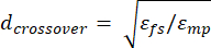    (2)

The energy utilization expected by the receiving node to get a data packet of m -bit is determined as follows:

    (3)

The mentioned model can determine the energy that the CH utilizes. The energy used by the CHs fundamentally incorporates three viewpoints: energy utilization of getting data packets of user nodes, associating information, and sending the fused information to the WR. The estimation formula is given as:

 (4)

The member nodes count is represented using CM_num, and E_DA is the expense required to aggregate 1 bit of data; the packet's length is m. The energy consumed by the non-CH hub is just the energy utilization of transmitting information to the WR, and the numerical formula is given as:

    (5)

The following is how the entire residual energy for the r^th round is computed:

 (6)

Where the entire remaining energy is given as in the round E_tohR(r - 1), the count of CHs present in the round is represented as CH_num(r), the N_alive(r) addresses total active nodes in the round of the provided network, E_Ch (i) represents the energy utilization of i^th CH and E_non-CH(j) indicates energy used by the non-CH(j).

Cluster selection
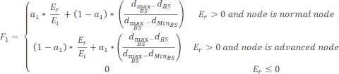
The algorithm utilizes the interspaces calculated from the node to the WR and energy to choose the primary clusters of the system, thereby restricting total CHs in clusters are as follows: According to the ascending fitness score of the SNs, the cluster of active SNs is partitioned into equal subsets of m (where m is the desired cluster count that is equivalent to N/p, N indicates the sensor nodes count and p CHs portion. In every subset, the first cluster head is chosen for the sensor node near the center position. Each node is added to the cluster head closest to it to create the initial cluster based on Euclidean distance. The space between the node, BS, and residual energy determines the node's fitness score.

  (7)

Where the weight is given as a₁, the primary energy is E_i, residual energy is given as E_r, and the space from the node to the WR is shown as d_BS. d_maxBS is the maximum inter-space between the SN and the WR, and d_MinBS indicates the minimum space between the SN and the WR.

Self-optimized wolf optimizer (SOWO)
The CHs are chosen using the SOWO. In the wolf optimizer, the location of the prey is identified using the average mass of the three wolves (α, β, and δ) as shown in Figure 2. Considering the differentiation among BS and the node and the space between the residual energy, the node's fitness score is regarded as the primary weight of the grey wolf optimization, which is determined using Equation (8). The initial location of the prey is calculated based on Equations (8) to (11) and the optimization technique of SOWO.

    (8)

    (9)

    (10)

    (11)

Where the primary mass of the wolves α, β, and δ are ω_Iα, ω_Iβ, and ω_Iδ respectively, the best fitness score for α wolf is F_α, F_β and F_δ which are computed using Equation 11. The individual nodes equivalent to the three highest fitness scores are α, β, and δ wolves. The developed protocol does not change the weight of the grey wolf optimization because the node's fitness score is changed after one data transmission is completed. To create the worldwide search capacity of the grey wolf optimizer, the loads are actively modified by vectors A and D. Here, A indicates the coefficient vector, and the remoteness from the wolf to its prey is D. Equations (12) and (15) are used to determine A and D. The position of the prey and the load upgrading formula are described as follows: the (t + 1)^th iteration:

  (12)

 (13)

 (14)

 (15)

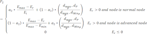
Where  specifies locations of the α wolf, β wolf, and δ wolf in the iteration (t+1), these locations  are computed using Equation (15). During the final stage of the iteration, the CH chooses which node is closer to the prey among the present nodes. The task of the CH is more complicated, so the residual energy cannot complete the task, which leads to the termination of the node. So, selecting the node with the maximum remaining energy and being nearer to the prey is essential. The node's remaining energy and the remoteness from the node to the prey are used as parameters for the fitness score used to choose the CH. The node with a lesser fitness score is identified as the cluster head. The function used to calculate the fitness value is given as:

  (16)

Where weight is given as a₂, node's remaining energy is represented as E_x, E_max is the maximum residual energy, and E_min is the minimal energy remaining in the cluster nodes. The distance between the prey and the node is d_p, d_Maxp is the maximum space between the detecting node and the prey, and d_Minp is the minimum space between the SN and the prey.

Self-optimization wolf agent
Software agents monitor and manage the network sizes and node gateways. The software agents replace traditional clients and servers, which differ in local communication strategy and code mobility. Monitoring is a crucial factor in understanding management systems. Due to this significance, software agent technology was suggested to monitor node gateways within the network mesh. In addition to monitoring, it is the responsibility of the agents to update the list of network nodes. This data is essential because of the network size, so the self-configuration process can dynamically configure the routing protocol parameters. In the context of this work, these are the most desirable characteristics among many found in the behavior of software agents. Wireless agents are installed at the client node associations of a mesh router and the router itself. In identifying the network density, the agent performs particular tasks on small, standard, and large scales. The scores for the three scales (small, standard, and large) are represented. The agents shape the premise of the auto-design capacity of the proposed protocols. These agents take responsibility for the network behavior verification, along with the throughput, data packet loss ratio, interruption, throughput, idleness, dynamic and dormant hubs, and data about the connection. Network agents are stable at the mesh routers and provide the proposed protocols' self-optimization capability. Self-association emerges in network remote organizations by implanting self-x capacities (optimization, setup, fix, and security¹⁹) in the routing protocol. These capabilities enable routing protocols to be autonomous, improving network performance, failure tolerance, and protection. The following is a description of the execution of the mentioned capabilities, with an emphasis on self-configuration and self-optimization. Notably, self-functions have been executed in network layers as extensions of standard services for routing protocols (Supplementary File 1).

Cluster set (CS)
CS is a collection of multiple clusters in a network, and the clustering algorithm allows for dividing a network into various clusters. In this research, the first chosen clusters are called the first CS, considered the present ideal CS, and the present perfect CS's objective function score is computed. Modified Grey Wolf Optimizer (MGWO) can arbitrarily modify all the clusters in the present perfect CS to produce another cluster, and a majority of the newly formed clusters frame another CS; again, the objective function score of the latest CS is determined. When the objective function score of the present optimal cluster is greater than that of the newest cluster, the newly determined cluster is taken as the present ideal CS. The perfect CS is framed toward the termination's final stage. The objective function is described as:

(17)

Where weight is represented as a₃, the sum of the space between the clusters in the CS is given as d_TCH and the entire remoteness between the CH and the WR is shown as d_TBS. The cluster and communication distance between the CH and the BS are the foundation for remote monitoring and target tracking design. If the objective function score is lower, then it demonstrates that the cluster head determination is more sensible, the CH is ideal in the cluster, and the cluster headset is perfect compared with the entire network. Algorithm 2 (Supplementary File 2) describes the SOWO pseudocode.

Results

Here, MATLAB R2024a compares the developed heterogeneous routing protocols using simulations with routing protocols. In the simulation, the network of 100 detecting nodes is arbitrarily employed with a dimension of one node every 100 m. The WR nodes are located in the network at (50 m, 120 m) and (50 m, 50 m). Roughly 20 percent of homogeneous nodes with (m as 0.2 and as 1) have less energy than the heterogeneous nodes. After the deployment, all of the nodes remain stationary. The simulation variables used in th...

Discussion

The proposed SOWO utilizes WRs and homogeneous nodes. The stable election protocol uses heterogeneous nodes as CHs and contains a BS node in the middle of the cluster surrounded by the sensor nodes. Increased energy is required if the base station is placed external to the region¹⁴. This leads to reduced energy, and the energy level reaches zero in a very short period. The proposed technique has a low energy reduction rate compared to traditional methods. This proves that the energy conservation m...

Materials

List of materials used in this article

Name	Company	Catalog Number	Comments
12th Gen Intel(R) Core(TM) i5-1235U (1.30 GHz)	Intel Corporation, USA	–	Hardware used for simulation execution
16 GB DDR4 RAM	Kingston Technology, USA	–	Memory used during simulation runs
MATLAB	MathWorks USA	R2024a	Used for implementing algorithms, running WSN simulations, and analyzing results
Microsoft Windows 11 Home	Microsoft Corporation, USA	Build 22631	Operating system used to run simulations
Synthetic Dataset Generated in MATLAB	MathWorks, USA	R2024a	Custom dataset created for algorithm testing

References

- Chowdhury, S. M., Hossain, A. Different energy saving schemes in wireless sensor networks: A survey. Wireless Pers Commun. 114 (3), 2043-2062 (2020).
- Hassan, M. B., et al. An enhanced cooperative communication scheme for physical uplink shared channel in NB-IoT. Wireless Pers Commun. 120 (6), 2367-2386 (2021).
- Noh, J. H., Park, J. H., Park, J. S. Data transmission direction based routing algorithm for improving network performance of IoT systems. Appl Sci. 10 (11), 3784(2020).
- Ahmed, R. A., Saeed, N. G., Sheetal, M., Amitava, M. Energy Optimization in LPWANs by using Heuristic Techniques. LPWAN Technologies for IoT and M2M Applications. , Elsevier. Amsterdam. (2020).
- Ahmed, M. K., et al. Optimizing energy consumption for cloud Internet of Things. Front Phys. 8, 358(2020).
- Sherubha, Graph-based event measurement for analyzing distributed anomalies in sensor networks. Sådhanå. 45, 212(2020).
- Sherubha, An efficient network threat detection and classification method using ANP-MVPS algorithm in wireless sensor networks. Int J Innov Technol Explor Eng. 8 (11), 1-8 (2019).
- Sherubha, An efficient intrusion detection and authentication mechanism for detecting clone attack in wireless sensor networks. J Adv Res Dyn Control Syst. 11 (5), 55-68 (2019).
- Mokhtar, R., Saeed, R., Alsaqour, Y., Abdallah, Y. Study on energy detection-based cooperative sensing in cognitive radio networks. J Netw. 8 (6), 1255-1261 (2013).
- Trong, D., Thi-Kien, H., Mong, S., Chin-Shiuh, S. An energy-based cluster head selection algorithm to support long-lifetime in wireless sensor networks. J Netw Intell. 1 (1), 23-37 (2016).
- Moridi, M., Sharifzadeh, Y., Kawamura, Y., Jang, H. D. Development of wireless sensor networks for underground communication and monitoring systems (the cases of underground mine environments). Tunn Undergr Space Technol. 73, 127-138 (2018).
- Huang, Z., Chen, T., Han, X., Liu, X. One energy-efficient random walk topology evolution method for underground wireless sensor networks. Int J Distrib Sens Netw. 14 (9), 155014771880062(2018).
- Priyadharshini, S. S., Nandhini, M., Gunasekaran, M. Energy-efficient multipath routing for wireless sensor networks. Int J Sci Technol Res. 9 (2), 1-6 (2020).
- Homogeneous and heterogeneous energy schemes for hierarchical cluster based routing protocols in WSN: A survey. Jagadeeswara Reddy, M., Suman Prakash, P., Chenna Reddy, P. Proceedings of the Third International Conference on Trends in Information, Telecommunication and Computing, 150, Lecture Notes in Electrical Engineering 501-508 (2013).
- Wu, X., Zhou, Q., Huang, Q. Optimal data routing algorithm for mine WSNs based on maximum life cycle. IEEE Access. 8, 131826-131834 (2020).
- Kathiroli, K., Selvadurai, K. Energy-efficient cluster head selection using improved sparrow search algorithm in wireless sensor networks. J King Saud Univ Comput Inf Sci. 34 (10), 8564-8575 (2022).
- Jibreel, E., Tuyishimire, M., Daabo, M. An enhanced heterogeneous gateway-based energy-aware multi-hop routing protocol for wireless sensor networks. Information. 13 (4), 166(2022).
- Nurelmadina, M., et al. A systematic review on cognitive radio in low power wide area network for industrial IoT applications. Sustainability. 13 (1), 338(2021).
- Shaikh, M. S., et al. Coverage and connectivity maximization for wireless sensor networks using improved chaotic grey wolf optimization. Sci Rep. 15, 15706(2025).
- Shaikh, M. S., et al. An intelligent hybrid grey wolf-particle swarm optimizer for optimization in complex engineering design problem. Sci Rep. 15, 18313(2025).
- Shaikh, M. S., et al. Applications, classifications, and challenges: A comprehensive evaluation of recently developed metaheuristics for search and analysis. Artif Intell Rev. 58, 390(2025).
Access restricted. Please log in or start a trial to view this content.