EasyFiji: A Graphical Interface for User-Friendly Fluorescence Image Processing in Fiji

Summary

EasyFiji is a graphical user interface plugin for Fiji (ImageJ) that provides a curated suite of fluorescence image visualization and processing tools frequently utilized by life scientists.

Abstract

Fiji (Fiji Is Just ImageJ) is an extensive and extensible open-source image processing package widely employed by the bioimage analysis community. However, for non-computational life scientists, manually interacting with Fiji's many capabilities requires learning and navigating a deeply layered menu system. Moreover, some commands' default behaviors are non-ideal for fluorescence image display and processing. To increase efficiency for life scientists working with fluorescence microscopy images, we have developed EasyFiji, a curated graphical user interface (GUI) plugin for Fiji. Each EasyFiji command is executed via tooltip-enhanced buttons and sliders and always exhibits channel-specific execution, as required for fluorescence images. Commands that alter pixel intensities are also single-click undoable to enable more interactive processing and can be automatically recorded and saved as text for record keeping. An image info panel displays settings crucial for image interpretation. New image rendering and bleach correction functions are also provided. The plugin is freely available on GitHub and as a Fiji Update Site. This protocol outlines the steps to use EasyFiji's interface for visualization and processing of fluorescence microscopy images.

Introduction

Fiji (Fiji Is Just ImageJ) is an extensive and extensible open-source image processing package widely employed by the bioimage analysis community^1,2. Fiji's large code base of general-purpose algorithms, along with its macro language and plugin interface, can be conveniently leveraged by computational analysts to provide a solution for almost any image processing or analysis problem. However, for life science users with little computational experience, FIJI's >1,100 commands spread across a deeply layered dropdown menu system can be dauntingly complex to navigate and utilize effectively. Several approaches have been taken towards simplifying the manual use of Fiji. Fiji's search bar is an alternative to menu navigation, providing access to excellent help documentation, but only if the user knows the name of the algorithm they need. Fiji's toolbar buttons can be customized to provide rapid access to user-defined commands, but this procedure requires writing a macro code and foresight of which commands will be most useful. The ActionBar plugin provides a standalone graphical user interface (GUI) window with customizable and organizable arrays of buttons but again, coding and experience are required to populate the buttons effectively³. None of these solutions satisfy the needs of life scientists with little image processing experience.

Beyond user interface issues, many life scientists working with fluorescence microscopy images require channel-specific display and processing procedures. However, some commonly utilized Fiji commands are not channel-aware by default. For example, users may want to render pseudo-colored channels together in either an equally salient way, or to specifically highlight regions of similar intensity between channels, or to preserve the grayscale contrast of a morphological signal while also displaying fluorescence. In each of these use cases, Fiji's RGB composite rendering technique obscures the desired information at the perceptual level. When processing multi-channel images, native Fiji image filters (i.e., Process | Filters), either process only the active 2D bit plane or else all bit planes in the image window (i.e., the 'stack' as defined by class ImageStack). The first behavior fails to process across the z- or t- dimension for a given channel, while the second behavior is almost invariably improper, since each channel contains a unique staining pattern and signal-to-noise ratio, necessitating the use of channel-specific processing parameters. Native Fiji's bleach correction commands (Image | Adjust | Bleach Correction) act incorrectly when applied to multi-channel fluorescence images, because again, they correct across the entire ImageStack, where channel data is interleaved, rather than correct across the z-or t-dimension within each channel individually.

To address these issues for life scientists working with fluorescence microscopy images, we have developed EasyFiji, a curated and guided graphical user interface plugin for Fiji. EasyFiji is a curated set of thematically organized commands that enable channel-aware rendering and processing. Four tabulated panels, Display, Process, Save, and Image Info, each contain topically related collections of tool-tip-enhanced buttons and sliders for command execution. Other conveniences include an undo functionality for interactive processing, a simple, plain-text action recorder that can automatically save pixel-modifying actions along with an image, and a formatted display of acquisition settings important for image interpretation. EasyFiji also offers new image rendering and bleach correction tools. EasyFiji does not support quantitative image analysis or batch-processing functions, as these procedures should only be performed with the help of an expert bioimage analyst. Although EasyFiji is concise by design, all native Fiji commands are always available through the native Fiji menu system. We believe that EasyFiji's audience-targeted design⁴ will increase the use of Fiji amongst life scientists. Here we present EasyFiji's design, implementation, and application to fluorescence microscopy images. The plugin is easy to install via a Fiji update site (https://imagej.github.io/list-of-update-sites/ and https://imagej.net/plugins/EasyFiji_plugin), while open-source code can be downloaded via GitHub; the plugin and source code are freely available (https://github.com/stjude/EasyFiji). 

Protocol

This protocol describes how to install and use EasyFiji.

1. To install EasyFiji…

1. Download the latest version of Fiji (>1.54g) appropriate for the operating system and install it in a folder to which the user has read/write access (see the Table of Materials for a link to the Fiji download site).
2. Launch Fiji and navigate to Help | Update… in the menu bar.
3. In the Updater window, click Manage Update sites. Select EasyFiji from the list, and click Apply and Close. EasyFiji will be automatically installed, and Fiji will be automatically updated with future releases of EasyFiji.
4. Restart Fiji. Select EasyFiji from the Fiji Plugins menu.
   NOTE: EasyFiji is fully compatible with many older versions of Fiji and is mainly compatible with ImageJ. Detailed compatibility and dependency information can be found on the EasyFiji GitHub wiki page (https://github.com/stjude/EasyFiji) and EasyFiji ImageJ.net wiki page (https://imagej.net/plugins/EasyFiji_plugin#quick-start). Feedback can be provided via the GitHub page or the EasyFiji thread on the Image.sc forum (https://forum.image.sc/t/announcing-easyfiji-a-user-friendly-gui-plugin-for-fiji/117617) (see Table of Materials for links to these resources). 

2. Using the EasyFiji display panel

NOTE: As shown in Figure 1A, the Display panel supports fluorescence channel pseudo-coloring using color swatch buttons, intuitive contrast adjustment controls, and new options for perceptually calibrated multi-channel image renderings. Native Fiji commands for 3D/4D image projection and re-slicing are also included. Table 1 documents the correspondence between EasyFiji commands and native Fiji commands.

1. Set a channel's color or visibility (Display Panel, Channel Color section).
   1. Select the desired channel using the image window's channel slider.
   2. Press a color swatch button to assign a new color lookup table (LUT) .
   3. Press the black swatch button to turn off the display of a channel .
   4. Press the AllChs button to display all channels together at once.
   5. Press the EachCh button to display each channel sequentially, by scrolling the channel slider in the image window .
2. Set channel contrast within or between images (Display Panel, Channel Contrast section).
   1. To change a channel's display range (contrast), select the channel using the channel slider at the bottom of the image's image window.
   2. Move the display gain slider to specify the image pixel intensity (value shown to the right) to be displayed as the brightest value on the screen.
      NOTE: We use the term display gain to describe this action because it causes the channel to become linearly brighter, analogous to the effect of changing the gain on a detector during image acquisition.
   3. Press the display gain reset button to display the channel's maximum possible pixel intensity (as determined by its bit-depth) as the brightest value on the screen.
   4. Move the display offset slider to specify the image pixel intensity (value shown to the right) to be displayed as the darkest value on the screen.
      NOTE: We used the term display offset to describe this action because it sets the image's black level, analogous to the effect of setting the offset on a detector during image acquisition.
   5. Press the display offset reset button to set the image pixel intensity of zero to the darkest value on the screen.
   6. Press the AutoCh button to automatically adjust the display gain and offset.
   7. Press the AutoAll button to automatically adjust the display gain and offset for all channels.
   8. Press the Propagate button to transfer the display gain and offset settings from the active image to all other open images that contain the same number of channels.
3. Create a multi-channel display (Display Panel, Channel Views section).
   1. To render two fluorescence channels together as a color image, use the FF-prefixed buttons (fluorescence with fluorescence). To render fluorescence channel(s) and a morphological grayscale channel together as a color image, use the FG-prefixed button (fluorescence with grayscale). Renderings are created in a new image window.
      NOTE: Prior to creating any Channel View, first adjust the display gain and offset for each channel such that the signal of interest spans the display's dynamic range (section 2.2) and then apply these gains and offsets using the Apply Gain and Offset buttons in the Processing tab (section 3.2.3). Renderings will be non-optimal if the gains and offsets are not adjusted and applied.
   2. Press the FFColoc button to produce a color rendering from two fluorescence channels that highlights as yellow pixels where the intensity is similar in both channels (within 25%).
      NOTE: Pixels with dissimilar intensities between channels are rendered in grayscale. Yellow pixels are suggestive of correlation-based colocalization⁵ when the signal of interest on each channel spans the display's dynamic range.
      CAUTION: The FFColoc rendering is intended solely for data exploration or illustration purposes. It is not a substitute for rigorous quantification of colocalization with the help of an expert.
   3. Press the FFMerge button to produce a color rendering from two fluorescence channels, where the signal in each channel is equally perceptible.
      NOTE: At each pixel, the luminance is set according to the signal with the higher intensity, while the hue is a function of the ratio of the intensities between the channels (following the concepts described by Taylor et al.⁶). See also the Discussion section.
   4. Press the FGMerge button to produce a color rendering from fluorescence channel(s) and a grayscale channel, where the coloration of the fluorescence channels is retained, while the contrast of the grayscale channel is retained.
      NOTE: The grayscale channel is typically a non-fluorescent modality containing morphological information, such as DIC, phase contrast, or electron microscopy.
   5. Press the Montage button to split the channels into individual images, automatically tile them across the screen, and synchronize their visualization.
   6. Press the SyncWins button to synchronize the visualization of multiple images of the same type.
4. Create 2D views of a 3D z- or t-stack (Display Panel, Stack Views section).
   NOTE: Each rendering is displayed in a new image window.
   1. Press the MIP button to create a maximum intensity projection.
      NOTE: The intensity at each location in the resulting 2D image corresponds to the intensity of the most intense pixel along the 3^rd dimension in the 3D image. This procedure can accentuate noise, so it can be useful to smooth the stack (see Processing tab) prior to creating a MIP.
   2. Press the SIP button to create a sum intensity projection.
      NOTE: The intensity at each location in the resulting 2D image corresponds to the sum of the intensities along the 3^rd dimension in the 3D image. This procedure preserves total intensity, resulting in a less noisy image than any single slice.
   3. Press the Ortho button to create an orthogonal slices viewer, which interactively renders the three orthogonal planes of a 3D stack (e.g., xy, xz, yz) that intersect at the current cursor location.
   4. Press the Kymo button to create a kymograph.
      NOTE: A kymograph is a 2D image where the vertical (y-) axis corresponds to a stack's third dimension (usually t-), and the horizontal (x-) axis corresponds to position along a line drawn by the user on the input stack. When the 3^rd dimension is time, a kymograph is used to illustrate or quantify motion.
      ​This button relies on the KymographBuilder plugin⁷ that comes with Fiji but must be downloaded separately if using ImageJ.
5. Set miscellaneous options (Display Panel).
   1. Press the Dup button to duplicate the active image window within Fiji. A new image window will appear.
      NOTE: Draw a rectangular region of interest (ROI) on the image using Fiji's Rectangle ROI tool, and the Dup button will crop to the ROI boundary. Specify channel, z-, and/or t- ranges to reshape the duplicated image's dimensionality.
   2. Press the ToClip button to copy the active image as currently displayed on the screen to the system clipboard. To paste the image into another application (to prepare slides or edit photos), make the other application active and select paste (Ctrl+V on Windows or Cmd+V on Mac).
   3. Press the |--um--| button to display a scale bar on the image as an overlay. Toggle the |--um--| button to remove the scale bar.

3. Using the EasyFiji Process panel

NOTE: As shown in Figure 1B, the Process panel Channel Features section provides slider-based image processing commands with tooltips that can be used to enhance image display. The Undo Last button enables interactive processing. Image dimensions can be changed using the Modify Dimensions buttons. The Action Table is used to log as plain text Processing commands that change image pixel intensity values. The log can then be automatically saved with the image using the same title (see Save panel).

1. Alter an image's spatial features (Process Panel, Modify Channel Features section).
   NOTE: All commands apply only to the active channel, and the results are automatically shown in the original image window. A new image window is not created.
   1. Move the Smooth slider to apply a Gaussian blur, thereby reducing normally distributed pixel-to-pixel variation (~shot noise and read noise).
      1. For ~Nyquist sampled images (70-150 nm xy pixel size), start with slider values between 1.0 and 2.0.
      2. For a given pixel size, increase the slider value as the image's signal-to-noise ratio (SNR) decreases.
      3. Given an SNR, increase the slider value as the pixel size decreases.
      4. For image stacks, apply a 3D smoothing, where the z-radius is automatically set to one-third the xy radius, as appropriate for Nyquist-sampled data.
         NOTE: The slider value corresponds to a Gaussian kernel's standard deviation measured in pixels.
   2. Move the Denoise slider to apply a median filter, thereby removing extreme outliers (camera hot pixels or PMT thermionic emissions).
      NOTE: The slider value corresponds to a box kernel's radius in pixels. Values between 0.5 and 1.0 are a good starting point.
   3. Move the Sharpen slider to apply a 2D unsharp mask, thereby reducing blur or haze, such as can be caused by out-of-focus light. Sharpening also accentuates noise.
      NOTE: The slider value corresponds to a Gaussian kernel's standard deviation (in units of pixels) used to define the scale of the blur. For ~Nyquist-sampled images (70-150 nm xy pixel size), slider values between 2.0 and 4.0 are a good starting point. The weight parameter is fixed at 0.6.
2. Alter image pixel intensities (Process Panel, Modify Channel Intensities section).
   NOTE: All commands apply only to the active channel, and the results are automatically shown in the image window. A new image window is not created.
   1. Move the Sub.Bkgd. slider to apply the 'rolling ball' algorithm, thereby removing background (i.e., spatially gradual intensity changes).
      NOTE: The slider value is the radius of the rolling ball in pixels, so larger values will subtract less total background. Value depends on image content but generally should be ≥2x larger than the size (measured in pixels) of the features to be preserved. Values between 10 and 20 are often a good starting point.
   2. Move the Gamma slider to enhance visualization of weaker signals mixed with brighter signals, such as may be needed to emphasize fine structures when intermixed with large structures.
      NOTE: After normalization, each pixel's value is raised to a power (exponent) given by the slider's value. Value depends on image content, but values between 0.6 and 0.8 are often a good starting point.
      CAUTION: Images where gamma has been applied cannot be used for intensity quantification.
   3. Press the Apply Gain and Offset: ToCh button or ToAll button to map the image display range (as specified by the display gain and offset sliders in the Display panel) onto the full range of intensities provided by the image's bit-depth.
      NOTE: This process is also known as applying lookup table (LUTs). The display Gain and Offset must be applied in this way prior to creating Channel Views in the Display panel.
   4. Use the Intensity Correction buttons to correct for artifactual intensity changes across the z- or t- dimensions of 3D images, such as could be caused by photobleaching, aberrations, or light scatter.
      NOTE: The action is applied to only the active channel. Local and global corrections can be applied sequentially to the same dataset. See the Results section for further explanation of the underlying methods.
   5. Press the Global buttons to correct for gradual signal intensity losses that occur across the entire z or t dimension, while preserving most biologically-driven intensity changes. There are two options:
      1. Press the GlobalL button to correct z-stacks where the initial slices may be dark or black, and the total intensity loss from first to last frame is mild (<50%). The algorithm models the intensity loss as a linear trend and then applies a correction factor to each slice such that the slope of the fit line becomes zero.
      2. Press the GlobalP button to correct time series where the first frames are the brightest and total intensity loss from the first to last frame is substantial (50%-95%). The algorithm models the intensity loss as a 2^nd order polynomial trend and then applies a correction factor to each slice such that the fit curve is transformed into a line with a slope of zero.
   6. Press the Local button to correct localized, abrupt signal intensity changes, while preserving gradual changes.
      NOTE: Such changes may be caused by bleaching of a few planes within a larger z-stack or by excitation power fluctuations (flicker). The algorithm models biologically relevant intensity changes as a fourth-order polynomial and then applies a correction factor to ensure that the median intensity of each frame equals the value of the fitted curve.
   7. Press the Equalize button to make the median signal intensity of each frame equal, similar to Fiji 'simple ratio' bleach correction method.
      CAUTION: Equalize may be useful for visualization purposes when all other methods fail, but it will erase biologically relevant variations in median intensity and so cannot be used in concert with intensity quantification.
3. Change an image's dimensionality (Process Panel, Modify Dimensions section).
   NOTE: These commands apply to all channels in the image window and cannot be reversed using the Undo button.
   1. Press the Rotate button to rotate the image, such as may be needed to align the anatomical axes of an embryo or tissue with the page or screen.
   2. Press the Crop button to reduce the image's xy dimensions. Look for the rectangular ROI tool that is automatically selected, and observe the prompt to draw an ROI on the image that will be used for cropping.
   3. Press the Subset button to create a new image stack from a subset of the input image's non-xy dimensions.
      NOTE: This is used to remove channels and/or to truncate slices in z or t.
4. Record the processing commands applied to an image (Process Panel, Record Actions section).
   NOTE: The purpose of the Action Recorder is to automatically log actions as plain text and then save the image with the applied actions, which change pixel intensity values. The log is a convenience so that the user does not have to manually take notes or decipher the Fiji macro recorder entries. Commands that do not change pixel intensities are not logged.
   1. Press the Rec button to start command recording.
      NOTE: The button face reads 'ON' when the recorder is recording. Executed commands and associated parameters will appear in the Action Table. Commands that are 'undone' are removed from the table.
   2. Press the Clr button to clear the Action Table.
   3. Press the Save button to save the Action Table as a text file. If actions applied to multiple images have been recorded, the actions will be grouped according to image title when the text file is saved.
      NOTE: Alternatively, save an image using the Save panel (section 4 below). Check the Save Actions box and all actions applied to the image will be automatically saved as a text file using the image's name and file path.

4. Using the EasyFiji Save Panel

NOTE: As shown in Figure 1C, the Save panel is designed to aid non-experts in selecting the correct image file format for their intended use case. When the Save Actions checkbox is checked, all processing actions applied to an image, as listed in the Action Table, are automatically saved with the image, using the same filename and path, except with a *.txt extension. If multiple images are open and were processed in parallel, all actions performed on all images are displayed in the Action Table. However, only the actions applied to the image being saved are saved with that image. The saved text file appears in the file system but does not open in Fiji. If desired, text files can be opened in Fiji by dragging the file icon onto the Fiji toolbar.

1. Save an image (Save Panel, Saving Methods section).
   1. Press the Raw Data button to save the image as a *.tif file, where exact pixel values, channel structure, and some metadata are preserved. Use this option when the goal is to further quantify or analyze an image.
   2. Press the Save for Presentation button to save the image as currently displayed using jpeg compression for the purposes of emailing or using in a slide presentation.
      CAUTION: This option should never be used for creating figures or for quantitative analysis.
   3. Move the Quality Level slider to set the jpeg compression level.
      NOTE: Larger values correspond to better preservation of pixel intensities and features (and larger file size), but never are all features preserved.
   4. Press the Save for Figure button to save the image as currently displayed in png format compatible with other graphics programs (e.g., Photoshop, Illustrator, Publisher, or GIMP). The image is saved as displayed on the screen, but channels and metadata are not preserved.
      CAUTION: This option should never be used for quantification.
   5. Press the Save as Movie button to save an image stack as an mov format movie that plays through the slices sequentially (z or t).
      NOTE: Playing mov files on a Windows-based operating system requires the open source VLC Media Player.

5. Using the EasyFiji Image Info panel

NOTE: As shown in Figure 1D, the Image Info panel displays plain text vendor-specific acquisition settings that are crucial for image interpretation. See Table 2 for a list of the types of confocal image formats that are currently supported.

1. Press the Channel Info button to load acquisition settings.
2. See the Channel Info section for channel-specific acquisition settings, including % laser power, laser wavelength, emission bandpass(es), gain, and pinhole size.
3. See the System Configuration section for image-wide settings, including system name, objective, scan mode, dwell time, and voxel size.

Results

Pseudo-colored renderings of multi-channel fluorescence images can be used to illustrate the spatial or intensity relationships between signals; however, native Fiji offers only an RGB composite rendering technique that inherently confounds coloration and brightness at the perceptual level. To illustrate this issue, Figure 2 uses a two-channel image of N-Myc and RNA Polymerase II (RNAPolII). In Figure 2A, each channel is displayed separately as grayscale so that no (possibly confounding) chromatic information is present. In Figure 2B, the channels are displayed together as Fiji RGB composite renderings, using all possible combinations of primary and/or secondary colors. As can be seen, different colored renderings convey very different information at the perceptual level (quantified below). Thus, the information perceived in a Fiji RGB composite rendering depends arbitrarily on which colors are assigned to which channels. Scientific renderings should be designed to convey specific information effectively.

Life scientists may desire a multi-channel rendering to assess the overall (spatial and intensity) relationship between two signals, where each signal is equally perceptible, independent of the coloration used. EasyFiji's FFMerge button provides such a rendering by coloring and merging the signals using the perceptually calibrated Commission Internationale de l'Éclairage (CIE LAB) color space⁸. Figure 2C shows two alternative FFMerge renderings of the channels in Figure 2A. As can be seen, both renderings appear to convey equal information about both signals, and this information is independent of the order in which the colors are assigned (quantified below).

To quantify these visual impressions, we computed the perceptual contrast present in each rendering. We measured perceptual contrast by computing each rendering's luminosity (using the Fiji LAB Stack command) and then taking the ratio of the luminosity's standard deviation to its mean. FFMerge renderings exhibited the largest perceptual contrast (0.25), while the Fiji RGB composite blue-green and blue-red renderings also performed well (0.25). The Fiji yellow-magenta and yellow-cyan renderings showed the least perceptual contrast (~0.15). To measure how this contrast corresponds to information about the input channels, we next used Pearson's correlation coefficient (PCC) to compare each rendering's luminosity to the luminosity of each channel when displayed alone as grayscale. Renderings where each channel is equally perceptible will show a similar level of correlation to each channel alone. (The individual channels have a low PCC value of 0.34 with one another). The ratio of the highest correlated channel to the lowest correlated channel is then a measure of perceptual bias, where a ratio of 1.0 indicates no bias. A ratio > 1.0 indicates that information about one channel predominates in the multi-channel rendering. The FFMerge renderings exhibited the least perceptual bias, with a ratio of 1.03, followed by the Fiji yellow-cyan renderings at 1.08. The Fiji blue-green and blue-yellow renderings exhibited the most bias with a ratio of ~2.3. Thus, only the EasyFiji FFMerge renderings exhibit both good perceptual contrast and low perceptual bias.

Life scientists may also want to visualize where two signals are qualitatively co-localized, meaning that both signals have a similar (normalized) intensity at the same pixel locations. (No qualitative display is a substitute for quantification, see Discussion). Traditionally, this need has often been fulfilled using the same Fiji red-green composite rendering described above, based on the premise that perception of yellowish pixels is attributable to colocalization, since yellowish corresponds to the equal or nearly equal presence of red and green (also termed the 'dye overlay technique')⁹.

To test the premise that perceptually yellowish colors in a Fiji red-green composite rendering indicate qualitative colocalization, in Figure 3A, left panel, we produced the spectrum of colors present in a Fiji red-green composite rendering. The white "V" outlines those colors corresponding to qualitative colocalization (i.e., the normalized intensity on both channels is within ±25%). To quantify how these colors are perceived, we then converted this spectrum into the LAB color space and graphed each color's luminosity (middle panel) and perceptual distance from pure yellow (right panel). The perceptual distance graph shows that intense, but non-colocalizing greens (colors northwest of the white V) are perceptually ~2x as close to pure yellow compared to equally intense, but non-colocalizing reds (southeast of the white V sector). Moreover, some of these non-colocalizing greens are perceptually closer to yellow (<40 units) than are colocalized yellowish pixels of moderate intensity (>50 units). These results indicate that some predominantly green, non-colocalizing colors are perceptually difficult to distinguish from truly colocalized yellowish pixels. Thus, the native Fiji red-green composite rendering results in perceptual confusion between colocalized and non-colocalized pixels and should not be used for visually judging qualitative colocalization.

EasyFiji's FFColoc button creates a color rendering that illustrates qualitative colocalization by highlighting colocalized pixels as yellowish (consistent with tradition) while avoiding perceptual confusion via rendering non-colocalizing pixels as grayscale. (Again, no qualitative display is a substitute for quantification, see Discussion). Figure 3D, left panel, shows the spectrum of colors produced by the FFColoc rendering, where again, the white "V" outlines colors corresponding to qualitative colocalization. Again, we converted this spectrum into the LAB color space and graphed each color's luminosity (middle panel) and perceptual distance from pure yellow (right panel). The right panel shows that in the FFColoc rendering, most colocalizing colors (those within the V) are chromatically closer to yellow (<40 units) compared to ~all non-colocalizing colors (>70 units), and that the non-colocalizing colors (either above or below the V) are equally distant from the colocalizing colors, reducing the possibility of perceptual confusion.

We further examined the use of the Fiji red-green composite rendering as a colocalization display using a two-channel image of the highly colocalizing synaptic markers Cerebellin-1 and Ionotropic Glutamate Receptor D2 (PCC = 0.83, Mander's Overlap Coefficient (MOC) = 0.92; Figure 3B). The Fiji red-green composite rendering of these signals is shown in the upper left panel of Figure 3C. For comparison, we also synthetically modified the signals to reduce their colocalization (PCC = 0.58, MOC = 0.73) as shown in the lower left panel of Figure 3C. Consistent with the quantitative results above, visual comparison of the Fiji composite renderings of the strongly and weakly colocalized signals shows that the strongly colocalized data is more yellowish, but differences at the level of individual puncta are hard to discern. This perceptual confusion is extreme for people who are color blind, as shown in the right panels of Figure 3C by using a color-blindness simulation (protanopia; created using the Fiji Simulate Color Blindness command).

We next applied the FFColoc rendering to the same two channels (repeated in Figure 3E). The FFColoc renderings of the strongly and (synthetic) weakly colocalizing signals are shown in the left panels of Figure 3F. In these renderings, the strongly colocalized signals are perceptually more yellowish overall than the weakly colocalized signals, and these differences are still perceptible at the level of individual puncta. Moreover, the FFColoc renderings are equally perceptible and distinguishable when observed by a color-blind person (since no red or green is present to be distinguished).

Finally, life scientists may like to overlay pseudo-colored fluorescence channels with a grayscale morphological signal (such as differential interference contrast (DIC), phase contrast, or scanning/transmission electron microscopy (EM), such that the grayscale contrast is preserved. Figure 4A illustrates this use case using a fluorescently stained cell culture combined with DIC. Figure 4B shows these channels displayed together using the Fiji RGB composite rendering technique. The contrast of the DIC channel in the Fiji rendering appears severely washed out. To quantify this effect, we computed the luminosity of the composite renderings and then used PCC to compare each rendering's luminosity to the luminosity of the DIC channel alone. The luminosity of the Fiji yellow-cyan-magenta rendering showed a low PCC with the DIC alone (0.48), while the luminosity of the Fiji red-green-blue rendering showed a modest PCC (0.67), indicating much information about the DIC channel is lost in both renderings.

The EasyFiji FGMerge button is designed to render together colorized fluorescence channels and a grayscale morphological channel with minimal loss of information from the grayscale channel. Figure 4C shows FGMerge renderings of the same channels used above. Again, PCC was used to compare the FGMerge rendering's luminosities to the luminosity of the DIC channel alone. The FGMerge yellow-cyan-magenta display showed a high PCC with the DIC alone (0.93), while the FGMerge red-green-blue display showed a good PCC with the DIC alone (0.80), indicating more information about the DIC channel is preserved in the FGMerge renderings than in the comparable Fiji composite renderings.

Figure 4D-F makes the same comparisons, only now in the context of correlative light and electron microscopy, where two fluorescence channels are combined with a backscatter SEM image. Figure 4D shows the channels alone, while Figure 4E shows these channels rendered together using the Fiji RGB composite technique. In this case, the colors happen to be non-overlapping, so the rendering's luminosity often remains well correlated with the SEM image alone (correlations: cyan-yellow 0.72; magenta-green 0.85; blue-red 0.98. See Discussion for why the blue-red combination performed well). Figure 4F shows the same channels rendered using the FGMerge technique. Here, the FGMerge rendering's luminosity is usually even more highly correlated with the SEM image alone than in the analogous Fiji RGB composites (cyan-yellow 0.99; magenta-green 0.93; blue-red 0.84), indicating that more morphological information is perceptible.

Another visualization problem encountered by life scientists working with fluorescence images is artifactual loss of signal across the z- or t- dimension of an image stack, often termed bleaching or decay. Signal loss can also occur locally, for example, if the user excessively dwells on one region prior to acquiring a volume or if excitation power is unstable over time. The native Fiji command Image | Adjust | Bleach Correction offers three methods to correct for global losses of signal intensity¹⁰ (see Discussion). Alternatively, EasyFiji provides three new intensity correction methods that are robust and channel-specific. Figure 5A shows a Gaussian light sheet z-stack of cells in an organoid that exhibits mild global bleaching (from right to left in the YZ view; detection objective was to the right) as well as strong local bleaching due to excessive light sheet focusing (the dark vertical stripe in the YZ MIP view). Figure 5B shows the stack after intensity correction using the EasyFiji GlobalL method to correct the global bleaching followed by the EasyFiji Local method to correct the local bleaching. The righthand graph of the median signal intensity versus slice number shows that both sides of the organoid 'shell' become equally intense after GlobalL correction, and the locally bleached stripe becomes nearly the same intensity as the surrounding slices after Local correction. Figure 5C shows that the native Fiji methods could not correct these intensity losses. At first, the native Fiji methods could not be directly applied to this dataset, because the signal was absent from the first frames and signal strength increased as a function of slice number. After solving these issues by removing the black frames and reversing the slice order, the Fiji Exponential method was executed, but the left half of the organoid became ~2-fold too bright, even more imbalanced than in the uncorrected raw data. The righthand graph quantifies these effects for both the native Fiji and EasyFiji GlobablL results.

As another example, Figure 5D-F shows a timelapse of migrating T-cells cells in culture. The YT views show that the signal exhibits modest bleaching over time (~50% total loss from first to last frame), while cells also migrate in and out of the field of view (Figure 5D). Figure 5E shows this dataset after intensity correction using the EasyFiji GlobalP method. The righthand graph quantifies that the GlobalP correction indeed resulted in the median intensity becoming constant over time. Figure 5F shows that the native Fiji Exponential method failed to correct for the intensity loss, despite that the loss followed an exponential-like decay (see Discussion).

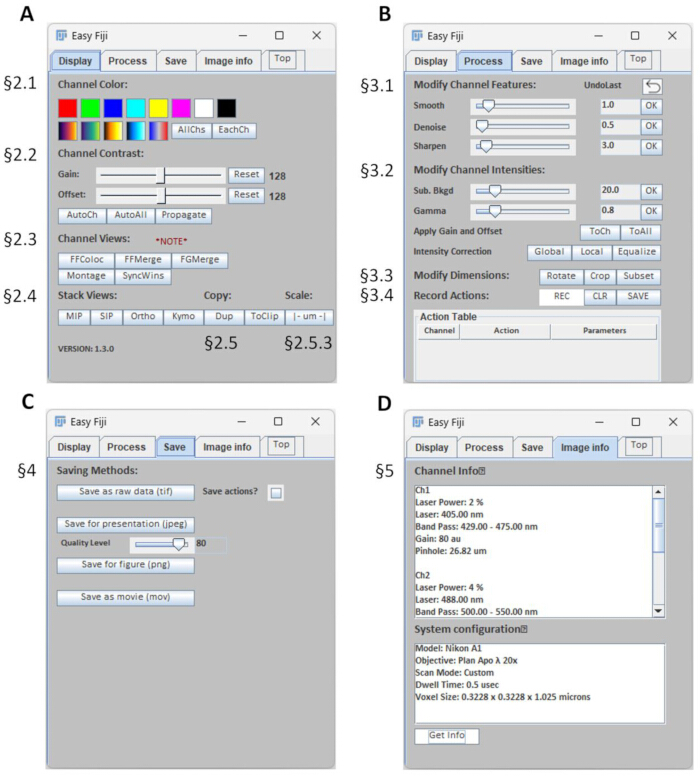
Figure 1. The EasyFiji graphical user interface. The plugin is thematically organized into four panels accessible via tabs: (A) Display, (B) Process, (C) Save, and (D) Image Info. The Top button makes the GUI always stay on top of other windows and can be toggled to float. (A) The Display Panel provides one-click access to common visualization tasks (2). The Channel Color section (2.1) provides swatches for assigning colors to channels or turning off a channel, as well as buttons to display the channels altogether or sequentially. The Channel Contrast section (2.2) provides sliders to set the black and white levels for channel display, buttons for auto-contrasting the active channel or all channels, and a button to propagate the contrast settings of the current image to all open image windows of the same type. The Channel Views section (2.3) provides techniques for rendering multiple channels together as a color image or splitting a multi-channel image into separate images for each channel. The Stack Views section (2.4) provides projections for 2D renderings of stacks. The Copy section buttons duplicate an image within Fiji (2.5.1) or copy it to the system clipboard (2.5.2). Scale section button adds a scale bar (2.5.3). (B) The Process Panel provides a suite of undoable slider-based and button-based image processing tools as well as an Action Recorder (3). The Modify Channel Features section (3.1) provides tools that smooth or sharpen image detail. The Modify Channel Intensities section (3.2) provides commands that modify an image's total intensity through background subtraction, linear or non-linear contrast adjustments, or global or local intensity correction across stack slices. The Modify Dimensions section (3.3) includes tools for re-shaping image dimensions or coordinates. The Record Actions section (3.4) enables plain text recording of processing commands that can be automatically saved with an image for record-keeping purposes. (C) The Save Panel provides methods for saving images in various use-case-oriented formats (4). (D) The Image Info Panel displays as formatted text channel-specific and system-level acquisition settings critical for image interpretation (5). Please click here to view a larger version of this figure.

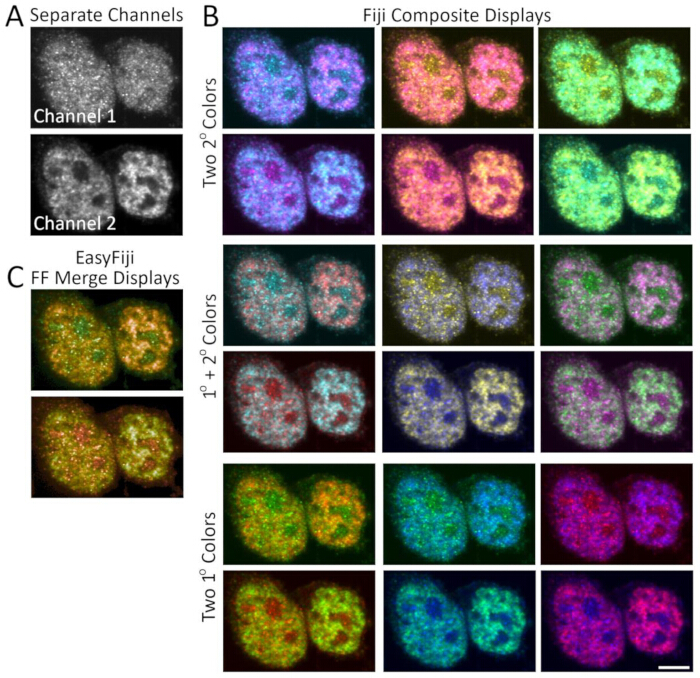
Figure 2. Native Fiji RGB composite renderings versus the EasyFiji FFMerge rendering for displaying two fluorescence channels together, such that information about both channels is equally perceptible. (A) Individual channels showing N-Myc and RNAPolII signals acquired using a Zeiss LSM780 with 63x NA 1.4 oil objective. Contrast was adjusted using the Display panel's Gain and Offset sliders to fill the display's range. The contrast was then applied using the Process tab's ToAll button. (B) Native Fiji RGB composite renderings assigning to each channel various combinations of secondary colors (top rows), primary and secondary colors (middle rows), or primary colors (bottom rows). (C) EasyFiji FFMerge displays of the same channels. Scale bar = 5 µm. Please click here to view a larger version of this figure.

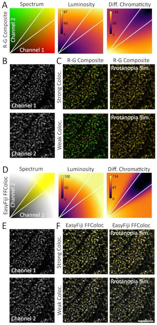
Figure 3. Native Fiji red-green composite rendering versus the EasyFiji FFColoc rendering for highlighting qualitatively colocalized pixels. (A) (Left panel) The color spectrum produced by the Fiji red-green composite rendering. The white "V" outlines channel intensity combinations near y=x, suggestive of colocalization. (Middle panel) The red-green composite spectrum's luminosity profile. (Right panel) The perceptual difference (based on LAB coordinates) between pure yellow and each other color in the red-green composite spectrum. Luminance and perceptual difference values are pseudo-colored using the mpl-inferno LUT. (B) Channels showing two synaptic markers that are strongly colocalized acquired using a Zeiss LSM780 with a 63x NA 1.4 oil objective. Contrast was adjusted using the Display panel's Gain and Offset sliders to fill the display's range. The contrast was then applied using the Process tab's ToAll button. (C) (Top row) The Fiji red-green composite rendering as perceived with normal color vision (left) or color blindness (right). (Bottom row) A synthetic, weakly colocalized version of the signals, rendered according to the Fiji red-green composite technique as perceived with normal color vision (left) or color blindness (right). (D) (Left panel) The color spectrum produced by the EasyFiji FFColoc rendering. (Middle panel) The luminosity profile of the FFColoc rendering's spectrum. (Right panel) The perceptual difference between pure yellow and each other color in the FFColoc spectrum. (E) The same synaptic signals as shown in B. (F) (Top row) The FFColoc rendering as perceived with normal color vision or color blindness. (Bottom row) The synthetic, weakly colocalized version of the signals, again rendered using FFColoc as perceived with normal color vision or color blindness. Scale bar = 5 µm. Please click here to view a larger version of this figure.

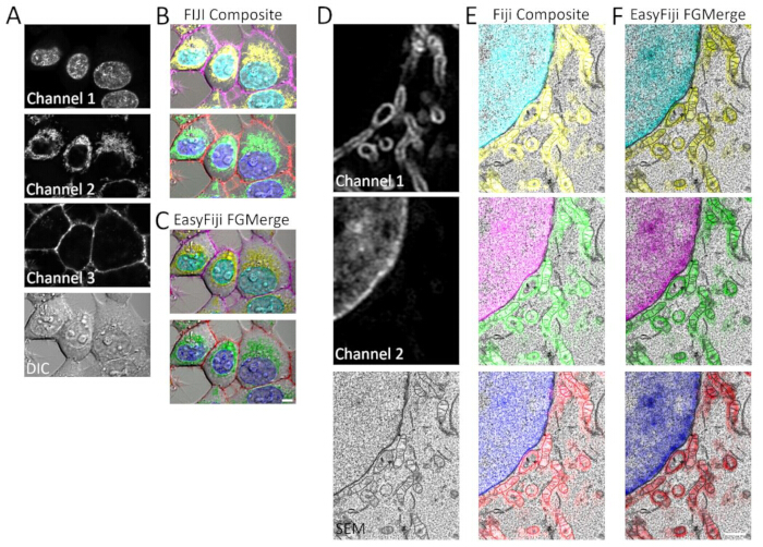
Figure 4. Native Fiji RGB composite renderings versus the EasyFiji FGMerge rendering for displaying together fluorescence channels and a morphological grayscale channel. (A) Three fluorescence channels and a DIC channel acquired using a Zeiss LSM980 with a 63x NA 1.4 oil objective. Contrast was adjusted using the Display panel's Gain and Offset sliders to fill the display's range. The contrast was then applied using the Process tab's ToAll button. (B) Fiji composite renderings of the fluorescence and DIC channels using different color combinations. (C) EasyFiji FGMerge renderings using the same color combinations. Scale bar = 5 µm. (D) Two fluorescence channels acquired using a Zeiss LSM780 with a 63x NA 1.4 oil objective and a backscattered SEM channel acquired using a Zeiss Gemini460 FEG SEM with 1.5 kV and 100 pA. Contrast was adjusted using the Display panel's Gain and Offset sliders to fill the display's range. The contrast was then applied using the Process tab's ToAll button. (E) Fiji composite renderings of the fluorescence and SEM channels using various color combinations. (F) EasyFiji FGMerge renderings using the same color combinations. Scale bar = 1 µm. Please click here to view a larger version of this figure.

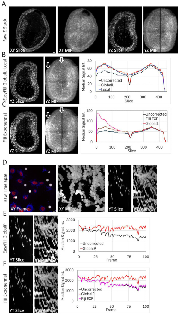
Figure 5. Native Fiji versus EasyFiji methods for intensity correction across slices in a z- or t-stack. (A) Cells in an organoid imaged using a Zeiss Lightsheet 7 microscope. Slice and maximum intensity projection views show a mild, systematic intensity loss from right to left in YZ orientation (detection objective was to the right), as well as severe local bleaching due to light sheet focusing (central dark line). (The subtle 'cross' pattern in the XY MIP is due to tile fusion artifacts during image stitching). Scale bar = 100 µm. (B) YZ Slice and MIP views after sequential application of the EasyFiji GlobalL and Local intensity correction methods. The graph shows the median signal intensity of each XY slice before correction, after GlobalL correction, and after Local correction. (C) YZ Slice and MIP views of the data after application of the native Fiji Exponential bleach correction method. The graph shows the median signal intensity of each XY slice before and after Fiji Exponential correction. The EasyFiji GlobalL correction result is included for comparison. (D) A timelapse captured once every three minutes of migrating immune cells (white) in cell culture acquired using a 3i W1 spinning disk confocal microscope with a 63x 1.2 NA water objective. Scale bar = 10 µm. The XY Frame shows a second cell type in red and blue to provide context, though only the immune cells were analyzed. Slice and maximum intensity projection views show a mild loss of intensity over time in the YT orientation. (E) YT Slice and MIP views after EasyFiji GlobalP correction. The graph shows the median signal intensity of each XY slice before and after GlobalP correction. (F) YT Slice and MIP views after application of the Fiji Exponential bleach correction method. The graph shows the median signal intensity of each XY slice before correction and after Fiji Exponential correction. The EasyFiji GlobalP correction result is included for comparison. Please click here to view a larger version of this figure.

Table 1. Correspondence between EasyFiji GUI elements and native Fiji menu commands. Icons in the first column represent EasyFiji GUI commands. The second column lists the corresponding sequence of native Fiji menu commands required to achieve the same outcome. Please click here to download this Table.

Table 2. Acquisition Metadata Displayed by the EasyFiji Image Info Tab. Each row in the first column describes an acquisition setting. Other columns correspond to file types, and entries indicate EasyFiji's support for each acquisition setting given each file type. The lower table shows the acquisition settings supported by Bioformat's OME-XML for comparison. User-provided file types will allow us to expand EasyFiji's support to camera-based systems, as well as other major vendors and models not available to us. Please click here to download this Table.

Discussion

Fiji is an open-source image processing and analysis software widely popular amongst image analysts. However, its complex menu interface and at times unintuitive behaviors relative to the display and processing of fluorescence images present challenges for non-computational life scientists. EasyFiji offers life scientists a curated set of thematically organized and tooltip-enhanced buttons and sliders that consistently exhibit channel-specific behaviors, as required when working with fluorescence images. All processing commands are undoable, enabling interactivity and can also be automatically recorded and saved with an image as plain text for record keeping. Acquisition settings critical for image interpretation are shown for Nikon and Zeiss point scanning confocals. Being a Fiji plugin, EasyFiji's conciseness is never a limitation, since all Fiji commands can always be accessed via the native Fiji menu system. In addition to the streamlined user interface, EasyFiji also offers several purposefully designed multi-channel rendering techniques as well as new methods for robust bleach (decay) correction. EasyFiji intentionally avoids providing quantitative analysis functions or batch processing, as quantitative image analysis should only be performed with the help of a bioimage analyst.

Although life scientists may combine multiple fluorescence channels into a color image for various reasons, native Fiji primarily provides a multi-channel RGB composite rendering technique. In this technique, the display coloration and brightness at each pixel are determined by summing the R, G, and B components of the color LUTs assigned to each channel. If a component's sum exceeds 255, the sum is clipped so as not to exceed the available bit-depth (see Fiji CompositeImage.java). (Pixel-wise 'either-or' displays are also available but do not provide information about both channels in the same pixel). However, as quantified in the Results, the Fiji RGB composite rendering is perceptually biased, depending arbitrarily on the colors used, because different RGB colors have different perceived brightnesses. EasyFiji provides several purpose-driven color rendering techniques, each geared towards a specific use case, that convey in a perceptually unbiased way more information about multi-channel fluorescence data.

The EasyFiji FFMerge button combines two fluorescence channels into a color image, ensuring that information from both channels is equally visible, regardless of the color assignments used. The FFMerge rendering is based on the perceptually calibrated CIE LAB color space, where colors are selected according to a polar coordinate system (a, b coordinates; white point being the origin) and L is the luminosity. In an FFMerge rendering, the angle in the a,b plane is determined by the ratio of intensities on each channel, and the color is then selected at a fixed radius for each luminosity (to stay within the sRBG gamut). The luminosity (L coordinate) is determined by the magnitude (norm) of the intensities on each channel. We used local contrast¹¹ and correlation measures to show that the FFMerge rendering exhibits both high perceptual contrast and low perceptual bias, unlike any Fiji RGB composite rendering.

The EasyFiji FFColoc button highlights regions of qualitative colocalization between two channels in a way that is equally perceptible to people with normal or abnormal color vision (color blind). The rendering is achieved using the HSB color space, where the hue is fixed at pure yellow, while the brightness set is according to the magnitude (norm) of the intensities on each channel, and the saturation is set according to the angle of the intensity's vector relative to the line y=x. We used chromatic distance measurements to show that the FFColoc rendering provides greater perceptual distinction between colocalized pixels and non-colocalized pixels than does a Fiji red-green composite rendering. FFColoc does not attempt to distinguish 'channel 1 alone' from 'channel 2 alone', because employing additional hues to distinguish the predominant channel reduces the perceptual distance to yellow. While graphical techniques to visualize colocalization in quantitative ways also exist, these methods require careful segmentation and choice of acquisition settings to be meaningful, and so should be applied only with the help of an expert^12,13. While not a substitute for quantification, the FFColoc display can help decide if a quantitative analysis is worth pursuing or can be used as an illustration in support of a quantitative analysis.

The EasyFiji FGMerge button provides a rendering of fluorescence channels with a grayscale morphological channel, whereby the grayscale channel's contrast is mainly preserved, while the fluorescence channel's coloration is preserved. These effects are achieved by rendering in the HSB color space, setting brightness according to the intensity of the grayscale signal, while hue and saturation are set according to the values in the colored fluorescence channels. When combining fluorescence and morphological grayscale channels, the native Fiji RGB composite rendering often results in contrast clipping due to high average grayscale values, and so loss of detail. The FGMerge rendering does not perfectly preserve grayscale contrast but typically exhibits higher luminance correlations with the grayscale channel (PCC > 0.90) than comparably colored native Fiji RGB composite renderings (PCC 0.5-0.8). The Fiji RGB composite rendering provided a higher correlation (0.98 vs 0.84) when blue and red colored channels where combined with an SEM image, but this case was unique because the colored channels did not overlap (and so never produced high luminance secondary colors), and the nearly white background in the SEM image was very luminous relative to the low luminance red and blue colors. A LAB color space rendering strategy (as used in the FFMerge rendering, except setting luminosity according to the luminosity of the grayscale image) would perfectly preserve grayscale contrast but would also be limited to rendering at most two colorized channels. We chose the HSB method, since its renderings provide high correlations with the grayscale channel in most cases and are compatible with any number of colorized fluorescence channels or heatmap LUTs, making it more broadly useful.

Another issue encountered with fluorescence images is artifactual loss of intensity across the third dimension of an image stack (z- or t-), often termed bleaching or decay, although this effect could arise through various mechanisms, including photobleaching, light scatter, or increased optical aberration as a function of imaging depth. While native Fiji provides bleach correction options, they are not robust in practice due to overly strong assumptions. First, the native Fiji methods use frame-wide average intensity as the basis for intensity correction; however, in practice, each slice of a stack typically contains a different fraction (by area) of signal-to-background. For example, in a z-stack, an object's cross-sectional area changes across slices, while during a time series, cells may enter or leave the field of view. Thus, frame-wide averaging confounds the signal's intensity with its prevalence (by area) in the frame. Frames may also contain no signal, for example, z-stacks are usually acquired 'black to black', and black frames can occur in time if all cells migrate out of the field of view or focus is temporarily lost. The mean statistic is also sensitive to the skewing of the signal's intensity distribution. Second, the native Fiji simple ratio and histogram matching methods assume that the signal's intensity distribution remains constant across frames; however, biologically relevant changes in signal intensity across z or t are the rule, not the exception. Consequently, these methods artifactually 'erase' any biologically relevant changes in the data. While the single exponential model preserves most biologically relevant changes, it assumes that intensity loss follows a single exponential, which is often not true due to the effects of the dye's local environment. Third, these native Fiji commands execute incorrectly without providing an error message when applied to multi-channel stacks, because they correct across the ImageStack data structure (where all channels are interleaved) rather than acting on each channel separately. As quantified in Figure 5, the native Fiji methods failed to correct intensity loss in an organoid because the spherical nature of the sample caused the percent signal in each frame to steadily decrease beyond the organoid's mid-point, thereby causing the frame-wide average intensity to decrease more rapidly than the signal's intensity per se, resulting in over-correction. The Fiji methods also failed to correct intensity loss across a timelapse of migrating cells, becausealthough the signal decayed exponentially as assumed, the signal-specific loss was offset by a frame-wide intensity gain due to more total cells entering the field of view across time. Thus, according to the frame-wide average intensity metric, intensity was nearly constant, and so virtually, no intensity correction occurred.

EasyFiji provides three new z or t-stack intensity correction methods that are channel-specific, robust, and make minimal assumptions. First, the EasyFiji methods use an automatic segmentation procedure based on an adaptive threshold to measure the median intensity of the signal per se. Measurements derived from frames where the signal occupies <2% of the total frame area are discarded. Second, the EasyFiji methods are model agnostic and instead use simple polynomial fits to describe trends in the data. The Global methods then correct each frame's intensity such that the slope of the fit line becomes zero (i.e., no change in median intensity across slices). The GlobalL method uses a linear model, while the GlobalP button uses a 2nd-order polynomial model. The linear model is best for preserving biologically driven local intensity changes but should only be used if the total intensity loss from first to last frame is <50%. (Larger magnitude losses are more likely to exhibit materially non-linear trends). The 2^nd-order polynomial model may remove some biologically driven changes but is more accurate for correcting substantial intensity losses (>50%), in part because it can closely approximate the curvature present in an exponential decay. The Local method corrects sudden intensity changes that occur over just a few frames and then recover. This method fits a 4^th-order polynomial to the median intensity data and then corrects the median intensity of each frame to match the value of the model. A 4^th-order model was used because it supports up to three inflection points, thus providing enough flexibility to model radially symmetric, 'shell-core' staining patterns without overfitting. The Local method can also artifactually erase biologically driven rapid intensity changes and should therefore not be used if these are expected. Global and Local corrections can be applied to the same dataset sequentially if needed. The Equalize method adjusts the median signal intensity across frames to be equal, similar to the 'simple ratio' native Fiji option. This method is useful when all other options have failed, and the primary goal is to visualize structures, rather than intensity per se, as this method will eliminate all biologically driven intensity changes.

EasyFiji offers an Action Recorder that automatically logs all pixel-intensity-modifying commands and parameters applied to the image as plain text and saves them with an image. Image specificity is maintained even if a command is undone (the command is then removed from the list) or if multiple images are open and being processed in parallel (only commands applied to a given image are saved with that image). Native Fiji's macro recorder logs all mouse clicks, including those extraneous to pixel-modifying operations, and produces executable code, but code-based logging adds much complexity for novice users to decipher, especially if multiple images are processed in parallel. The Fiji macro recorder output is also not automatically saved with the image that was processed. The EasyFiji Action Recorder is convenient for logging only those EasyFiji commands that modify pixel values, and so are important to note at the time of publication.

Finally, the EasyFiji Image Info tab displays formatted text acquisition settings that are critical for life scientists to interpret fluorescence images acquired on common commercial confocal systems. These settings include system name, objective, scan mode, dwell time, voxel size, % laser power(s), laser wavelength(s), emission bandpass(es), gain(s), and pinhole size. While only Zeiss and Nikon confocal files are currently supported, we plan to expand support to common camera-based systems and other common vendors in a future release, based on user feedback. Leica, by default, does not save metadata, and we did not have access to Olympus confocal files. Bioformats OME-XML metadata typically displays only two of the above settings, objective and voxels size, along with miscellaneous hardware information unrelated to image interpretation.

While EasyFiji is simple, concise, and curated by design, we welcome insightful user feedback and may incorporate additional features or simplifications useful to life scientists in future updates. Users may provide feedback via the EasyFiji GitHub page or EasyFiji Image.sc forum thread (URLs for these websites are listed in the Table of Materials).

Materials

List of materials used in this article

Name	Company	Catalog Number	Comments
EasyFiji GitHub Site	Open Source		https://github.com/stjude/EasyFiji
EasyFiji Image.sc forum	Open Source		https://forum.image.sc/t/announcing-easyfiji-a-user-friendly-gui-plugin-for-fiji/117617
EasyFiji ImageJ.net site	Open Source		https://imagej.net/plugins/EasyFiji_plugin#quick-start
FIJI Software	Open Source		https://imagej.net/software/fiji/downloads
VLC Media Player	Open Source		https://www.videolan.org/vlc/

References

- Schindelin, J., et al. Fiji: an open-source platform for biological-image analysis. Nat Methods. 9 (7), 676-682 (2012).
- Rueden, C. T., et al. ImageJ2: ImageJ for the next generation of scientific image data. BMC Bioinformatics. 18 (1), 529(2017).
- Mutterer, J. Custom toolbars and mini applications with Action Bar. Figshare. 10 (m9), (2017).
- Levet, F., et al. Developing open-source software for bioimage analysis: opportunities and challenges. F1000Res. 10, 302(2021).
- Aaron, J. S., Taylor, A. B., Chew, T. L. Image co-localization-co-occurrence versus correlation. J Cell Sci. 131 (3), (2018).
- Taylor, A. B., Ioannou, M. S., Watanabe, T., Hahn, K., Chew, T. L. Perceptually accurate display of two greyscale images as a single colour image. J Microsc. 268 (1), 73-83 (2017).
- Mary, H., Brouhard, G. KymographBuilder. , https://imagej.net/plugins/kymograph-builder (2016).
- Schanda, J. Colorimetry: understanding the CIE system. , Wiley Interscience. Hoboken. (2007).
- Dunn, K. W., Kamocka, M. M., McDonald, J. H. A practical guide to evaluating colocalization in biological microscopy. Am J Physiol Cell Physiol. 300 (4), C723-C742 (2011).
- Miura, K. Bleach correction ImageJ plugin for compensating the photobleaching of time-lapse sequences. F1000Res. 9, 1494(2020).
- Reid, R. C. Jr, Shapley, R. Brightness induction by local contrast and the spatial dependence of assimilation. Vision Res. 28 (1), 115-132 (1988).
- Stauffer, W., Sheng, H., Lim, H. N. EzColocalization: an ImageJ plugin for visualizing and measuring colocalization in cells and organisms. Sci Rep. 8 (1), 15764(2018).
- Taylor, A. B., Ioannou, M. S., Aaron, J., Chew, T. L. Model-free quantification and visualization of colocalization in fluorescence images. Cytometry A. 93 (5), 504-516 (2018).
Reprints and Permissions