Temperature Response of Soil Organic Matter Decomposition Rates: Construction and Applications of a Temperature Gradient Block

Summary

We introduce a temperature gradient block and detail its construction and utilization. The block provides 22 discrete temperatures, linearly distributed between a user-defined range from 0 to 90 °C. Data collected from this setup enables testing and developing new theories on the temperature response of soil organic matter decomposition rates.

Abstract

Soil is the Earth's largest carbon (C) reservoir, holding nearly twice as much C as the atmosphere. Climate change-induced temperature increases could enhance soil organic matter (SOM) decomposition, potentially releasing carbon dioxide (CO₂) into the atmosphere, thus resulting in a positive feedback to climate change. This presents the question: how can we define the response of SOM decomposition rates to short-term changes in temperature? Can we utilize this data to fit mechanistically defined equations in Earth system models for climate predictions? Most research to date has focused on laboratory soil incubations at different discrete temperatures. This, however, does not result in a detailed temperature response curve, which is required to test novel hypotheses imposed by the latest developments in the field, such as the macromolecular rate theory (MMRT). In this paper, we introduce a temperature gradient block, modified and improved from earlier work, detail its construction process, and provide a detailed explanation for its utilization. The temperature gradient block is an aluminum block with four rows of 22 discrete holes, allowing the simultaneous incubation of 88 microcosms (60 mL vials). The block is cooled at one end and heated at the other, creating a linear temperature distribution. It provides 22 discrete temperature points along a user-defined range within limits of 0 to 90 °C. After 3.5 h of incubation, CO₂ production is measured from each of the 88 microcosms. Results demonstrate that the block produces the user-defined temperature gradient and facilitates the construction of temperature response curves of SOM decomposition. Additionally, the data collected from this setup can be used to test and develop new hypotheses and theories regarding the impact of temperature changes on SOM decomposition rates, an area of increasing importance in the context of climate change.

Introduction

Increasing carbon dioxide (CO₂) concentrations in the atmosphere lead to higher temperatures on Earth¹. This phenomenon was first reported in 1856 by Eunice Foote², who conducted a simple yet groundbreaking experiment. She filled one cylinder with ambient air and another with CO₂ and recorded the temperatures in both¹. The results were clear: cylinders with higher CO₂ concentrations exhibited higher temperatures, demonstrating the warming effect of increased atmospheric CO₂¹. This observation has significant implications for climate change. Today, Foote's early insights continue to inform contemporary climate science, guiding research on how rising CO₂ levels affect global warming and influence various ecosystems.

Soils store nearly twice as much carbon (C) as the atmosphere in the first meter, playing a crucial role in the global C cycle³. A key process influencing soil C stocks is soil organic matter (SOM) decomposition, which determines the rate at which C is released back into the atmosphere^4,5. Higher mean annual temperatures, driven by climate change, have the potential to stimulate soil organic matter (SOM) decomposition, accelerating the release of CO₂ into the atmosphere^6,7. This represents a positive feedback mechanism to climate change, particularly when higher temperatures accelerate C losses through SOM decomposition more than they stimulate photosynthetic C inputs⁶. Despite extensive research on the topic, the magnitude and direction of the so-called land-carbon-climate feedback remains widely debated^8,9,10,11. This uncertainty is largely due to fundamental knowledge gaps regarding the temperature response of SOM decomposition rates. Addressing these gaps is essential for refining Earth system models and incorporating theoretically grounded representations of the temperature response of SOM decomposition rates.

The temperature response of SOM decomposition rates is commonly represented by the Q₁₀ value and the Arrhenius equation. The Q₁₀ value is defined as the factor by which a rate is multiplied when the temperature increases by  10 °C. Despite challenges to its validity^12,13,14,15, Q₁₀ has become the default approach for comparing the temperature response of different treatments and soils. The Arrhenius theory suggests an exponential increase in process rates, such as those of SOM decomposition, with increasing temperature¹⁶. However, actual enzyme activities tend to follow a unimodal form with a distinct thermal optimum and decline at higher temperatures^17,18,19. Arrhenius-based equations attempt to account for this decline by suggesting enzyme denaturation beyond the thermal optimum⁶. However, enzyme denaturation occurs at higher temperatures than those commonly found in soils, indicating that enzymes reach a thermal optimum before denaturation occurs^19,20. Moreover, simply adding a second function to the Arrhenius equation to account for the collapse of respiration rates due to denaturation does not allow estimation of an inflection point temperature - the temperature at which the rate of change in respiration is maximized^21,22. Consequently, Arrhenius-based equations fail to fully capture the commonly measured shape of the overall temperature response of SOM decomposition rates within the range of temperatures generally observed in soils^14,23.

To address the limitations of Arrhenius theory, multiple equations have been developed to represent the temperature sensitivity of biological processes; however, few are grounded in biological theory or have been applied to soils^24,25. Among the biologically-based approaches, the macromolecular rate theory (MMRT) overcomes some of the Arrhenius equation's limitations by incorporating the thermodynamic properties of biological macromolecules, such as enzymes²⁶. Similarly, the Enzyme-Assisted Arrhenius theory (EAAR) accounts for the temperature-dependent role of enzymes in lowering the activation energy of the reaction²⁴. Both equations have been successfully applied to studies of the temperature response of biochemical reactions in soils and microorganisms^17,24,27,28. These equations provide valuable mechanistic insights into the temperature response of SOM decomposition and underlying reaction steps. However, their broad adoption and parametrization are often hindered by experimental challenges.

Both field and laboratory studies have advantages and limitations for understanding the temperature response of SOM decomposition rates. Field experiments provide valuable insights on the long-term temperature response of SOM decomposition rates. However, interpreting CO₂ flux measurements in the field can be challenging due to confounding variables such as autotrophic respiration, moisture variability, and substrate accessibility^{29,30,31,32,33}. While these interactions are essential for quantifying real-world processes, such studies are generally focused on long-term ecosystem responses rather than the measurements of short-term mechanistic processes. Understanding the short-term temperature response is crucial for parameterizing equations that are defined by recent theories, like MMRT and EAAR, and for this, laboratory studies are key. Many laboratory studies typically suffer from confounding effects of substrate depletion, which increase with incubation time and temperature treatments^34,35,36. Additionally, most laboratory experiments use only a few temperature treatments^37,38,39,40, resulting in fitting simple exponential equations or calculating Q₁₀ ratios instead of more advanced equations, which require rates to be measured at a larger number of discrete temperatures⁴¹. To address these issues, it is crucial to develop new experimental approaches that enable accurate measurements of SOM decomposition rates across a broader range of temperatures, thereby supporting the rigorous testing and development of SOM decomposition theories in relation to temperature response.

In this paper, we describe the construction and utilization of a temperature gradient block, which not only addresses current experimental limitations but also provides a state-of-the-art study to demonstrate the short-term response of SOM decomposition to temperature. The design presented here is an adaptation of the methodology first developed by Thomas et al. (1963)⁴² and later modified by Robinson et al. (2017)⁴¹. The main differences include 1) an improvement of the cooling system, 2) a reduced operating time by coupling the block to a CO₂ analyzer for direct measurement of CO₂ concentrations, and 3) eliminating the need for transporting vials during the experiment. While previous reports^21,41,43 have provided a broad description of the temperature block, the detailed design, construction methods, and testing were minimal, limiting the ability for other researchers to utilize this approach. Here, we provide complete details of both the design and construction, and present results from multiple tests to demonstrate the proper functionality of the setup for different soil samples.

Protocol

Here, we present the detailed construction and in-depth utilization of the temperature gradient block. All the materials with their respective specifications can be found in the Supplementary Table 1 and Table of Materials. The cost of construction and assembly of the temperature gradient block was approximately €20,000, excluding the cost of the gas analyzer. This temperature gradient block is named 'Eunice' after Eunice Foote.

1. Construction of the temperature gradient block

1. Refer to Figure 1 for the body design of the temperature gradient block.
2. Constructing the aluminum block
   1. Position and secure the raw aluminum block in a universal milling machine. Input the measurements and locations for each hole into the machine's software. Figure 2 specifies the location and diameter of each hole for the setup.
   2. Drill holes for heating rods. On one end of the block, drill two holes with a diameter of 16 mm and a depth of 133 mm. Position these holes such that their centers are located 25 mm from the top edge and 36.25 mm from the side edges (Figure 2).
   3. Create a castle pattern for a cooling agent. At the opposite end of the block, drill a castle pattern over a length of 180 mm (Figure 3A). Ensure that the castle pattern has a thickness of 16 mm and a depth of 140 mm. Drill 12 additional holes within the castle pattern, each with a diameter of 10 mm and a depth of 140 mm. Refer to Figure 3B for the precise location and distribution of these holes.
      NOTE: The castle pattern was created to increase the contact of the cooling agent with the block, and the 12 holes serve to prevent overflow.
   4. Create a gasket for the castle pattern. Cut an aluminum gasket to enclose the cooling agent within the block and place it on top of the castle pattern. This is used to prevent leakage of the cooling agent.
   5. Drill holes for the cooler connection. On the front and back sides of the block, drill holes with a diameter of 15 mm for the cooler connection (Figure 4). Position the center of the holes at 75 mm depth. Ensure that the hole on the front side is 18 mm from the edge and the hole on the back side is 162 mm from the edge. Ensure that these two holes connect the start and end of the castle pattern.
   6. Drill holes for temperature sensors. Drill 8 holes with a diameter of 3 mm with a depth of 150 mm. These sensors are located in the middle of the block and evenly distributed along its length. Ensure that the center of the first sensor hole is 940 mm from the edge, and the last sensor hole is 205 mm from the edge.
   7. Drill holes for the 60 mL vials. Create 88 holes, each with a diameter of 28 mm and a height of 144 mm. These holes are evenly distributed across the block. The center of the first and last vial holes aligns with the centers of the first and last sensor holes.
3. Insulation preparation
   NOTE: The insulation material is made of polyisocyanurate with a thickness of 40 mm.
   1. Using a circular saw, cut the insulation material into a trapezoid shape at an angle of 135°. To cover the four long sides of the aluminum block, cut the insulation material into a rectangle measuring 1080 mm by 230 mm. Cut each of the four sides of this rectangle at an angle of 135° to fit snugly around the block. One of these sides will be glued to the lid of the block. Use aluminum tape to protect the insulation material for the lid of the block.
   2. For the two short sides of the block, cut the insulation material into a square measuring 230 mm by 230 mm. Again, cut each side of the square at an angle of 135° to ensure a proper fit.
4. Connecting the cooling system (Figure 5)
   NOTE: The cooling system used in this setup is compact and energy efficient. This cooling system is operated by circulating a natural cooling agent with a cooling capacity up to -30 °C.
   1. Attach the knee coupling and hose barb to the block (Figure 5C). Then, connect the hose that directs the cooling agent to the cooler.
   2. Cover the hose with flexible insulation material to cover the hose entirely. This will keep the cooling agent at the desired temperature. Cut the flexible insulation material and tightly fit it to the hose, using adhesive sealant to fix the insulation.
5. Insert the heating rod and sensors into the block to ensure the fit (Figure 5D).
6. Refer to Figure 5 for an overview of the steps explained above.

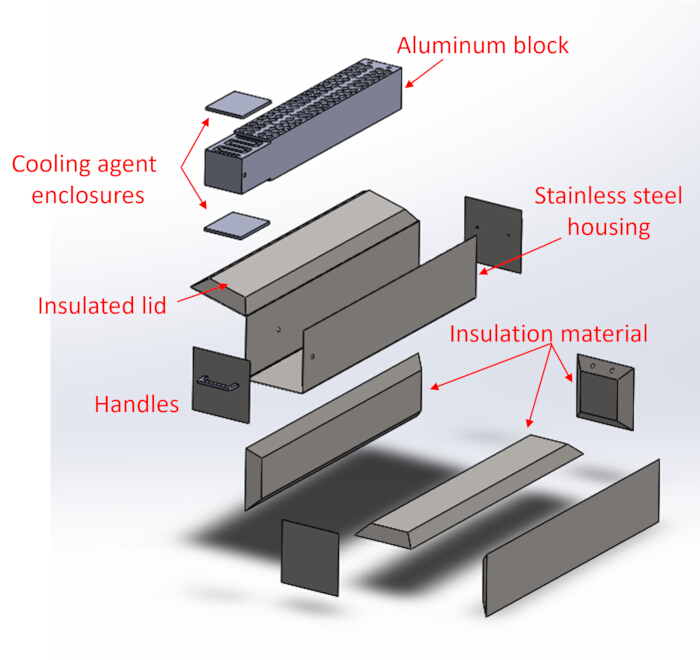
Figure 1: Body design and parts of the temperature gradient block. Please click here to view a larger version of this figure.

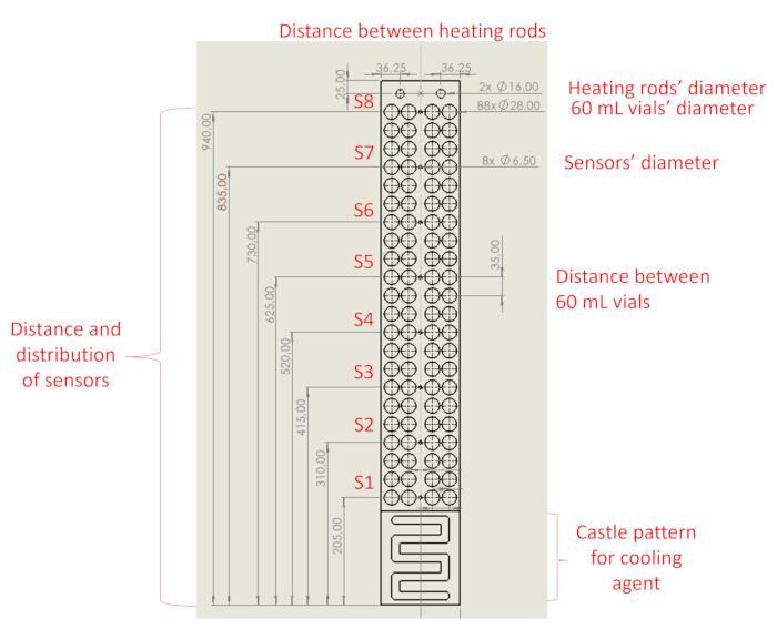
Figure 2: Temperature gradient block outlining the location and diameter of the holes used for multiple uses. Letter "S" denotes sensor. Dimensions are in millimeters (mm). Please click here to view a larger version of this figure.

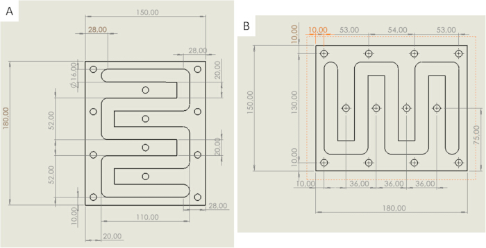
Figure 3: Design and measurements of the castle pattern used for the cooling agent. (A) Measurements of the castle pattern thickness, length, and diameter, and (B) distance and location of 12 holes used to prevent overflow. Dimensions are in millimeters (mm). Please click here to view a larger version of this figure.

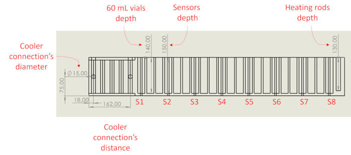
Figure 4: Side view of the temperature gradient block indicating the depth of each hole and location of the cooler connections. Letter "S" denotes sensor. Dimensions are in millimeters (mm). Please click here to view a larger version of this figure.

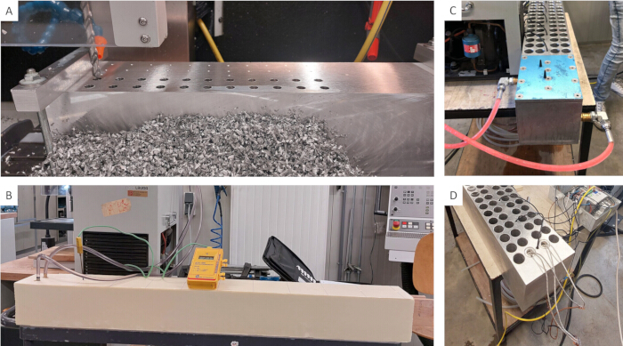
Figure 5: Overview of the construction of the temperature gradient block. (A) Drilling holes for placing the 60 mL vials; (B) building the insulation material covering the aluminum block; (C) connection and enclosure for the cooling agent; (D) inserting the heating rod and sensors into the block. Please click here to view a larger version of this figure.

2. Constructing the stainless-steel housing.

1. Cut the stainless steel for the long sides with the dimensions 1080 mm x 230 mm x 230 mm. For the short sides, cut the stainless steel with dimensions 230 mm x 230 mm. Make sure to make holes for the cooling hose, sensors, heating rods, and handles.
   NOTE: One of the long sides is used as the lid of the block.
2. Heat-connect the handles, hinges for the lid, and closures to the stainless-steel housing.

3. Construction of the electronics unit

NOTE: Only a qualified electrician may construct the electronic unit. The protocol outlined here has been developed in accordance with Dutch and EU laws. Below is a brief overview of the main components used; detailed wiring instructions are provided in Supplementary File 1.

1. Design the electronic diagram (Figure 6).
2. Mount the junction boxes.
   NOTE: The junction boxes are installed for the protection of the electric components and connections from external objects and damage.
   1. Securely mount the three junction boxes to the stainless-steel housing using the mounting screws.
   2. Prepared cable entry points. In the main junction box, knock out six holes for cable glands. In the two smaller boxes, knock out two holes for cable glands. One box will house the 2-way switch, and the other the heater rod cable connections.
      NOTE: The 2-way switch is used to turn on and off the unit, meaning that it provides power to the mini circuit breaker.
   3. In the main junction box, drill one hole on the top for the green LED.
      NOTE: This LED light indicates when the unit is on, and power is available to every component.
   4. Cut and fit the DIN rail into the main junction box. Then, mark out three holes for mounting screws that will hold the DIN rail. Mount the DIN rail into the main junction box.
      NOTE: The DIN rail is used to facilitate the mounting of the electrical components. Preferably, place it roughly in the center of the main junction box.
3. Electric components installation.
   NOTE: Use Figure 7 as a reference and install each electric component.
   1. Locate the junction box for the 2-way switch. Remove the top half of the switch to find the portion that needs to be fed through the cover plate. Mark and drill out a hole in the cover plate of the switch junction box, which needs to snugly fit and mount the switch to the cover plate. Use the switch mounting instructions.
   2. In the main junction box, place the PE/GND terminal on the DIN rail. Then, place the miniature circuit breaker (MCB) on the DIN rail.
      NOTE: The PE/GND terminals are used as end tops. The MCB is a miniature circuit breaker, and the main safety breaker in the event of a fault or shortage. When the MCB is on, it applies power to the AC/DC power supply.
   3. Place two triple feed-thru terminals on the DIN rail. Using two terminal double bridge terminals to join them at the top and bottom of the feed-thru terminals.
      NOTE: Use feed-thru terminals to connect more than two wires and utilize bridges to link multiple feed-thru terminals together. Ensure a secure and reliable connection by using the ferrule connectors.
   4. Place the DC power supply on the DIN rail as pictured.
      NOTE: This study used a 24 V, 2.5 A AC/DC power supply. Which uses the AC power and converts it to 24 VDC for the other components' input power requirements.
   5. Place the thermostat on the DIN rail as pictured. Ensure not to lose the cable connection module (Green in Figure 7).
      NOTE: A thermostat was used to control and monitor the temperature. It is a web-browser-based software system that requires the IP address of the unit to log-in and set the temperature of the heating rods, and record the data. This was connected to the local area network (LAN) to be able to connect to the unit from any computer on campus.
   6. Place seven triple feed-thru terminals on the DIN rail as pictured. Using three quintuple bridges, join the first five feed-thrus together at the top, middle, and bottom feed-thru terminals.
   7. Use two quintuple bridges to join the last two feed-thrus together at the top and bottom feed-thrus.
   8. Place one fuse holder on the DIN rail as pictured.
      NOTE: A 630 mA fuse was used to protect the unit components from damage in the event of short circuits and power surges.
   9. Place two single terminal connection units on the DIN rail as pictured.
   10. Place the solid-state relay on the DIN rail as pictured.
       ​NOTE: The solid-state relay is used to turn on and off the heating rods.
   11. Place one PE/GND terminal as the end stop.
4. For the electric wire connection procedure, refer to Supplementary Figure 1.
5. For an overview of the electronic unit, refer to Figure 7.

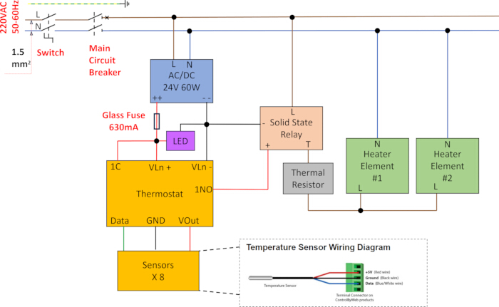
Figure 6: Diagram for the electronic unit. Wire colors are as follows: brown = Voltage Alternating Current (VAC) line, blue = VAC neutral, green and yellow = GND (Ground/Earth), red = Voltage Direct Current (VDC) positive, black = VDC negative. Data wires are white, but for ease of their identification, in this figure are shown in green color. Please click here to view a larger version of this figure.

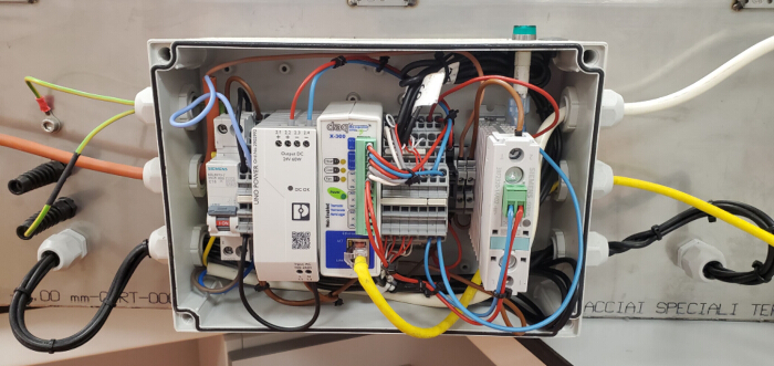
Figure 7: Main junction box of the electronic unit attached to the temperature gradient block. Please click here to view a larger version of this figure.

4. Assembling the temperature gradient block

1. Use adhesive sealant to glue the insulation material to the stainless-steel housing. Let it dry overnight.
2. Insert the sensors and heating rods inside the aluminum block.
3. Place the aluminum block inside the stainless-steel housing, guiding the cables through their respective holes for connection to the electronic unit.
4. Use the hinges to attach the insulated stainless-steel lid to the block.
5. Attach the cooling system to the aluminum block.
6. Place the temperature gradient block in the laboratory, ensuring all connections are secure and functional (Figure 8A). Ensure the laboratory has a sturdy table at least 2 m long. Confirm there is access to Ethernet and electricity connections. A controlled ambient temperature is desired for optimal operation.

5. Construction of the flushing system

NOTE: The flushing line was designed to standardize CO₂ concentrations in each vial at the start of the incubation. Refer to Figure 8B to visualize the flushing system with the temperature gradient block.

1. Cut the smaller diameter flexible tube into 10 pieces, each measuring 15 cm in length. Attach a needle to one end of each of the 10 smaller tubes.
2. Cut the larger diameter tube into a single piece measuring 1 m in length. Place a stopper at one end of this tube and connect the other end to the ambient air conductor in the lab.
3. Measure and mark the larger tube at 5 cm intervals along its length. At each marked interval, insert a needle connected to one of the smaller tubes.

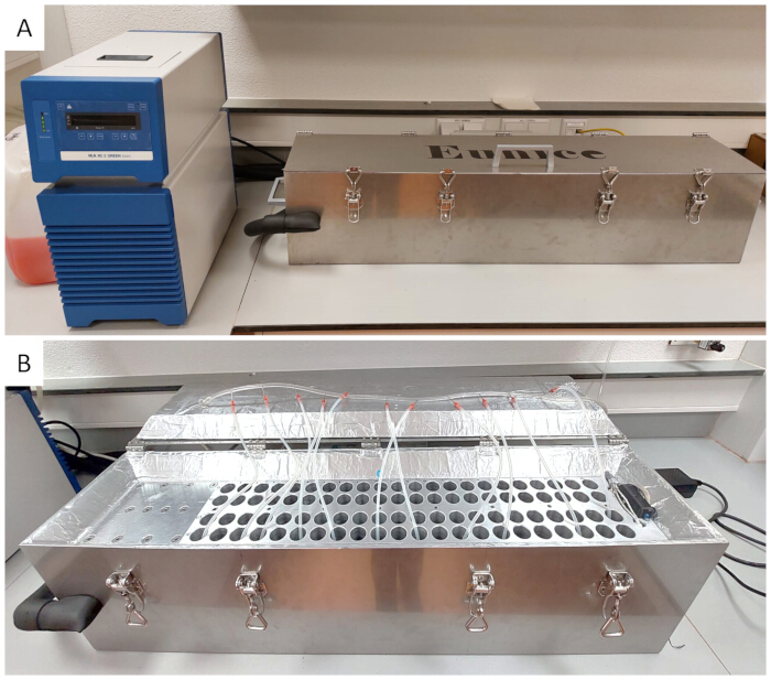
Figure 8: Temperature gradient block. (A) Temperature gradient block installed in the laboratory with the lid closed and (B) open with the flushing system in display. Please click here to view a larger version of this figure.

6. Description of the gas analyzer injection unit

NOTE: The gas analyzer of this setup allows for measuring CO₂ concentration directly in the 60 mL glass vials. The range for this gas analyzer is between 0 ppm and 10000 ppm with a precision of 0.04 ppm at 400 ppm. The gas analyzer comes with a flow reduction kit that measures at a rate of 1.17 mL/s.

1. Modify the injection tube of the gas analyzer by adding an external 0.45 µm filter and an injection needle (Figure 9).
   ​NOTE: The 0.45 µm filter was added as an additional precaution to avoid water entering the gas analyzer. The needle has a size of 18 G and dimensions of 1.2 mm x 25 mm. The needle was selected based on the diameter to minimize damage to the rubber septa of the 60 mL glass vials.
2. Connect the injection tube of the gas analyzer to the instrument's connection inlet.
3. At the end of the injection tube, attach a male Luer lock connector. Using a flexible tube with an internal diameter of 1/4, secure the Luer lock to the injection tube. Then, attach the 0.45 µm filter using a flexible tube to air-tight everything together.
4. On the screw end of the 0.45 µm filter, use a male and female connector to securely attach the needle.

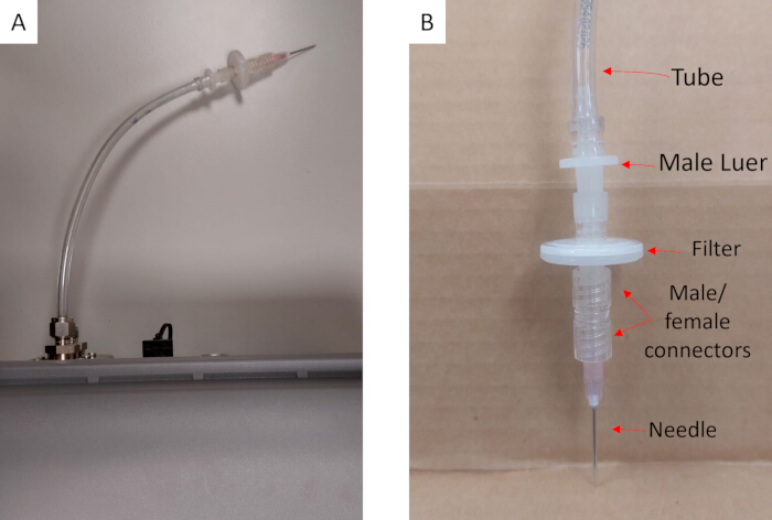
Figure 9: Gas analyzer injection unit. (A) The injection tube of the gas analyzer. (B) An external 0.45 µm filter and an injection needle. Please click here to view a larger version of this figure.

7. Designing treatments for incubation

1. Select soil samples.
   NOTE: The soil samples chosen for this manuscript demonstrate the protocol's functionality and showcase the type of data that can be collected using this setup.
2. Select a temperature range for block incubation, which is a user-defined range from 0 °C to 90 °C.
   NOTE: The temperature range for this manuscript was 4 °C to 60 °C. If the system is used beyond this range, follow laboratory safety protocols when handling high or subzero temperatures.
3. Plan the randomization of the samples.
   NOTE: For this manuscript, samples were randomized within the temperature block (positions A-D). Although this study initially tested randomizing the sample reading after incubation, this introduced labeling errors during the reading process. Therefore, a consistent measurement order (i.e., from high to low temperatures) was prioritized.

8. Preparing samples for pre-incubation

NOTE: To limit shifts in soil microbial communities, soil samples should preferably be incubated fresh as soon as possible after sampling. However, depending on experimental constraints and logistics, soil samples may need to be air-dried for transport and storage before incubation. In this manuscript, an air-drying procedure was standardized for processing samples before incubation.

1. Sieve the fresh soil using a 2 mm sieve. Let the sieved soil dry at 40 °C for 24 h. This air-dried soil can be stored until further processing.
2. Place the soil sample in a metal tin and mix it thoroughly. Distribute the mixed soil into 22 pre-labeled 60 mL glass vials. Using weighing paper, add 3 ± 0.03 g of soil into each 60 mL vial.
3. Using a pipette, adjust the soil to the desired water-holding capacity (WHC) based on the funnel method. After adjusting the water content to the target %WHC, record the exact weight of each vial.
   NOTE: The soil samples selected for this manuscript were adjusted to 60% WHC.
4. Cap the vials using cotton wool to allow for ambient air exchange.
5. Pre-incubate the samples for 10 days in a temperature-controlled lab at 20 °C.

9. Adjusting WHC during pre-incubation

1. After 7 days of pre-incubation, record the weight of the vials and adjust to the target WHC. Use a pipette to be precise and add water as needed. Calculate the water to add to each vial using Equation 1.
   Water to add = weight_T0 (g) - weight_T7 (g)   (1)
   where weight_T0 represents the weight of the vial at time zero and weight_T7 represents the weight of the vial after 7 days.

10. Initializing the temperature gradient block

NOTE: The cooling system is controlled using the panel in the front of the instrument. The heating system is controlled using the switch behind the instrument and an online interface.

1. Follow the instructions of the manufacturer to turn ON the cooling system. Press the power button once (Item A, Supplementary Figure 2). Ensure that the numbers for the Temp °C and the rpm should blink with the message OFF. This indicates that the system is ON but currently inactive.
2. Activate the pump by pressing the OK/Pump button (Item E, Supplementary Figure 2) and press the + or - button (Item G and F, Supplementary Figure 2) to set the rpm to 3500. Before activating the cooling system, check that the fluid level has green lights (Item L, Supplementary Figure 2). If the fluid level is red, this means there is not enough cooling agent. Contact the lab manager or refer to the manufacturer's manual.
3. Activate the cooling system by pressing Temp (Item B, Figure S2) and press the + or - buttons (Item D and C, Supplementary Figure 2) to set the Temp °C to -1.6 °C. The set point (Item O, Supplementary Figure 2) should be blinking. This indicates that the cooling system is not at the set point yet.
   NOTE: The set temperature in the cooling system is not the same as the temperature inside the block.
4. Turn the switch behind the block ON (Supplementary Figure 3). Ensure that a green light turns ON This indicates that the heating system is ON, but the temperature control is not active.
5. To activate the temperature control of the heating system, open the online interface of the temperature gradient block by entering the IP address 10.75.117.227 in a browser. Log in with the provided username and password to view the temperature of each sensor (Supplementary Figure 4). This interface shows the sensor values, which are updated every 3 s.
6. Adjust the Set Heating Temp to 60.00 °C by pressing the up/down arrows. Press the ON button to activate the heating system.
   NOTE: It takes about an hour for the block to reach a stable linear temperature gradient.
7. Ten minutes after the block has been turned ON, check the heater control to make sure it is working. The instrument is working when the temperature is different for each sensor.

11. Setting up the gas analyzer

1. Following the instruction manual of the manufacturer, turn ON the gas analyzer by pressing the power button once. Wait for 45 min for the instrument to warm up.
2. Connect the PC to the gas analyzer's Wi-Fi network, identified by the unique hostname (TG15-XXXXX) and use the password to connect.
3. Write the hostname or IP address in a web browser and press enter to connect. Then, open the settings section and select reduce flow rate. If the option is already selected, do not change anything in the software.

12. Getting ready to load samples

1. Adjust the WHC following section 6 of the protocol 1 h before starting the incubation.
2. Check the heater control to make sure it has reached the desired temperature 10 min before placing samples in the block.
3. Turn ON the ambient conductor located in the lab.
4. Connect the flushing system and connect the gas analyzer to the computer.

13. Collect blanks

1. Record blanks following these two procedures:
2. Connect the flushing line to the injection system of the gas analyzer and record the CO₂ (in ppm) of the flushing line directly.
3. Place five 60 mL glass vials in an empty holder. For each vial, place one flushing line. After 1 min, take the flushing line out and cap the vial. Wait for four hours before measuring CO₂ inside the vials.

14. Loading samples in the temperature gradient block

NOTE: In the block you will have block positions A, B, C, D. Place the same sample in the same block position across the block (Figure 10). For example, sample number 175 goes in block position A from 1 to 22, sample number 45 goes in block position B from 1 to 22, etc.

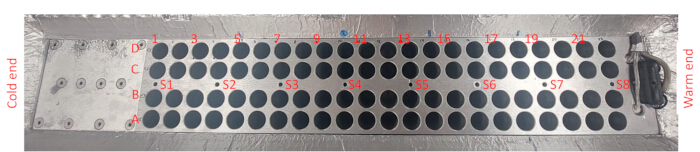
Figure 10: Vial positions inside the block. Letter "S" denotes sensor. Please click here to view a larger version of this figure.

1. Open the block, place the computer and flushing system on top of the block lid (Figure 11). On a movable table, place the boxes containing the samples.
   NOTE: Wear a KN95 mask to minimize CO₂ variability in the samples. This prevents CO₂ from the respiration from contaminating the vials.
2. Prepare a spreadsheet to record the closing time (hour: minute) of each individual vial, and in parallel, visualize the time of the gas analyzer.
   NOTE: The closing time of each vial is used for rate normalization during data processing.
3. Start loading the samples in the temperature gradient block. Work in batches of eight samples. Place the uncapped samples inside the block, starting from the cooler end. This means the first eight samples are A1, B1, C1, D1, A2, B2, C2, D2.
4. Place the flushing line in eight vials and wait 1 min. Take the flushing line out and immediately close the vials. On a spreadsheet, record the exact time each vial was capped.
   NOTE: Carefully insert the flushing line into each vial, ensuring it does not come into contact with the soil. This prevents cross-contamination and helps maintain sample integrity.
5. While the first eight vials are flushing, load the next batch of samples into the temperature gradient block. For example, the flushing samples are: A1, B1, C1, D1, A2, B2, C2, D2. The next batch of samples to be added are: A3, B3, C3, D3, A4, B4, C4, D4.
6. Place the flushing line into the next batch of samples.
7. Repeat these steps until the block is fully loaded.
8. Close the block and wait 3.5 h from the moment the last sample was closed.
9. Set the gas analyzer to Sleep Mode, by pressing the power button twice within 3 s.
10. Turn OFF the flushing system using the red valve located in the wall.

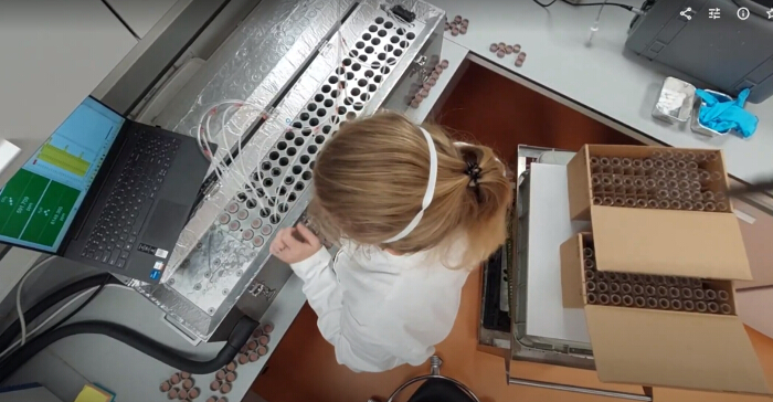
Figure 11: Loading temperature gradient block setup. Please click here to view a larger version of this figure.

15. Starting with CO₂ measurements

1. Take the gas analyzer out of Sleep Mode by pressing the power button once 1 h before starting with CO₂ measurements. Check the analyzer settings as indicated in section 8.
2. Turn ON the flushing system and place the gas analyzer onto the movable table (Figure 12).
   NOTE: The movable table has to be tall enough for the injection system of the gas analyzer to reach all the samples.
3. Check the diagnostic section of the gas analyzer (Supplementary Figure 5). Ensure that the status of the instrument is green for all components. Here, there are two possibilities:
   1. If everything is green, start the analysis.
   2. If there are red or yellow components, check the gas analyzer manual and, if necessary, ask for technical help. If the error is fixed, then proceed with the CO₂ measurements. If the error is not fixed, stop the experiment.
4. Open the graph section of the gas analyzer to visualize the real-time measurements. Keep in mind that the instrument is constantly measuring CO₂ from the air.
   NOTE: The measurement display is delayed for ~3-5 s.
5. After 3.5 h of incubation, start measuring the samples. Starting with the higher temperatures. For example, the first samples to read are: A22, B22, C22, and D22.
   NOTE: Wear the KN95 mask when measuring samples at temperatures <15 °C. This will reduce noise in the data.
6. Connect the injection needle of the analyzer to a flushing line between samples. This will make data cleaning easier.
7. On top of the screen, there is a REMARK function in the gas analyzer software. Every time a sample is measured, create a UNIQUE and SIMPLE remark. Do not forget to hit REMARK before running each sample.
   NOTE: Use unique numbers or the unique ID of the sample as a REMARK. If a mistake is made in the REMARK, take note of the time the sample was measured. For example, take notes of late injections, if the REMARK was ended early or late, etc.
8. Insert the needle in the 60 mL sample vial for 20 s. After these seconds have passed, take the needle out of the vial.
   NOTE: The gas analyzer will have pressure issues if the needle is left inside the 60 mL vial for more than 38 s. Avoid this because the gas analyzer will stop working for a few minutes, until the pressure stabilizes again.
9. Follow these steps for reading samples and the five blanks with the gas analyzer:
   NOTE: Hit the REMARK button in the online software of the gas analyzer to start and end a remark.
   1. Start REMARK at hh:mm:00.
   2. Insert the needle into the vial at hh:mm:10.
   3. Take the needle out of the vial at hh:mm:30.
   4. Stop REMARK at: hh:mm:45.
10. Change the 0.45 µm filter connected to the analyzer injection needle every 16 samples. This filter is meant to capture moisture and prevent clogging of the filters inside the analyzer.
11. Repeat these steps for all samples.

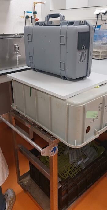
Figure 12: Place the gas analyzer on the movable table. Please click here to view a larger version of this figure.

16. Unloading samples from the temperature gradient block

1. One by one, take samples out of the block and place them in a box. Follow one of these options:
   1. Unloading while measuring CO₂.
   2. Unloading after measuring the last CO₂ sample.
      NOTE: Select one of the two options based on the requirements for future sample analysis after block incubation or the lab schedule. For instance, step 16.1.1 might change the incubation duration for some samples, which could impact the results of subsequent analyses. The lab schedule (e.g., opening and closing hours) could also be a limiting factor.
2. Process and store samples for future analysis.
   NOTE: In this case, all 88 samples were preserved after block incubation. Using a spatula, the entire sample was transferred from the 60 mL glass vial into pre-labeled plastic bags.

17. Downloading the data

1. To extract the data collected with the gas analyzer, go to the online software of the gas analyzer. Click on Settings and then hit the Download icon.
2. Select the specific time the first and last sample were measured. Click Download.
3. Open a new spreadsheet, select Open File. Change the file search to All files (*.*) and look for the document saved in the previous step. A new window will open, then select Finish.

18. Turning off the instruments

1. Power off the gas analyzer with the power button or through the software interface. To power off the instrument with the button, press the Power Off button three times within 5 s.
2. Turn OFF the cooling system. Press lock (Item I, Supplementary Figure 2) and the OK/Pump button (Item E, Supplementary Figure 2). The white noise should stop. After the white noise is completely gone, press the OFF bottom.
3. Turn OFF the heating system. Switch off the temperature gradient block control system using the switch behind the instrument. Make sure the green light turns OFF (Supplementary Figure 3).

19. Converting CO₂ ppm to respiration rates in µg C per kg soil per hour

1. Import the gas analyzer data into postprocessing software (we used R), and extract the following variables: REMARK, TIME, CO₂, and H₂O.
2. Create a new column to extract the seconds of interest, specifically from >30 s to <35 s.
3. Remove any observations that have pressure drop-related problems. During the experiment, pressure drops may have caused slightly lower CO₂ readings than expected. These slight drops (between 3% and 5% lower than the previous or next value) are not real changes in CO₂, but rather artifacts (errors) caused by pressure drop. Therefore, remove CO₂ values that have dropped slightly (~3-5%) compared to the previous or next CO₂ value.
4. Calculate the average CO₂ concentration (ppm) for the remaining data points. For each sample, subtract the mean of the five measured blanks.
5. Import the lab data into postprocessing software (e.g., R), and extract the following variables: REMARK, dry soil weight, and closing time.
6. To convert the CO₂ ppm measured by the analyzer to µg C per g soil, apply Equation 2:
   
   where CO₂ concentration measured by the gas analyzer is expressed in ppm; CO₂ molecular weight is equal to 44.01 g·mol^-1; P is the barometric pressure, is equal to 1 and expressed in atm; R is the universal gas constant equal to 0.082058 expressed in atm·mol^-1·K^-1; head space is calculated based on the head space of the 60 mL glass vials expressed in mL; T is the assumed internal temperature of the instrument, equal to 293.15 and expressed in K; and dry soil weight is expressed in g.
7. Then, divide by the incubation time expressed in hours and multiply by 1000 to convert grams to kilograms of soil.
8. Lastly, convert the µg CO₂ to µg of carbon using the molecular weights of CO₂ and C. This will result in respiration rates expressed in µg C per kilogram of soil per hour.
9. Save or export the processed data for further analysis.

Results

Stability and distribution of the block temperature
During the development of this protocol, we tested the linearity and temporal stability of the temperature inside the block. After switching the cooling system and the heater ON, the initialization time of the block is approximately one hour, during which time most of the eight evenly distributed temperature sensors reach the target temperature and then remain constant after an overshoot (Figure 13A). After this period, the temperatures recorded by the eight sensors confirm a perfect linear distribution of the temperature along the aluminum block (Figure 13B).

Figure 13: Linearity and temporal stability inside the temperature gradient block. (A) Temporal stability of the temperatures inside the block over the incubation period, and (B) temperature recorded by the sensors at the starting time of the incubation. Please click here to view a larger version of this figure.

Block temperature and soil temperature
We tested the time required for the soil sample inside the block to reach the temperature recorded by the eight sensors (Figure 14). In this study, we measured the temperature of soil samples at eight different positions within the block, located near the sensors. The sensors, positioned inside the block were pre-stabilized at their target temperature. Following the above-described protocol, once the block temperatures were stable, soil samples were placed inside the block. For this test, we used extra sensors that are separated from the block. We used 15 g of soil, ensuring that the sensor probe was in full contact with the soil. The soil samples were left uncapped, and the temperature was recorded every minute for a total of 30 min. During this test, the block was slightly closed to minimize temperature variation and reproduce as much as possible real utilization conditions (completely closed). We found that it takes approximately 12 min for the soil samples to stabilize at the target temperature. We deemed this stabilization time to be acceptable, given that the incubations last for a minimum of 3.5 h. Additionally, we assessed the linearity of soil temperature after 12 min of block incubation. The results indicate that the soil temperatures exhibit a linear relationship, closely aligning with the linearity observed in the eight sensors (Figure 15).

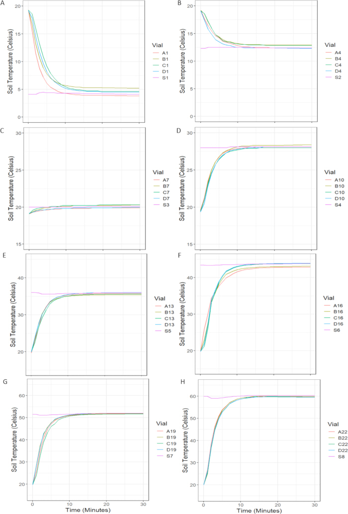
Figure 14: Recorded soil temperature incubated at different temperatures. Samples A, B, C, and D were incubated in vials positioned near the corresponding sensors (see Figure 10 for reference). The soil temperature was recorded by a thermocouple inserted directly into the soil samples. The specific temperatures monitored by each sensor are as follows: (A) Sensor 1 (S1) at 4.1 °C , (B) Sensor 2 (S2) at 12.5 °C, (C) Sensor 3 (S3) at 20.1 °C, (D) Sensor 4 (S4) at 28.1 °C, (E) Sensor 5 (S5) at 36.1 °C, (F) Sensor 6 (S6) at 43.8 °C, (G) Sensor 7 (S7) at 51.9 °C, and (H) Sensor 8 (S8) at 60 °C. After placing the soil samples into the block, it takes approximately 12 min to reach the target temperature. Please click here to view a larger version of this figure.

Figure 15: Strong linear correlation between soil temperature and sensor temperature. Four vials with soil were placed close to the eight sensors in block positions A, B, C, and D. The soil temperature was recorded by a thermocouple inserted directly into the soil samples. Please click here to view a larger version of this figure.

Temperature-moisture interaction
There is an inevitable interaction between temperature and moisture that needs to be assessed during the incubation period. For instance, high temperatures can accelerate evaporation, while low temperatures can cause water condensation. For this test, we used four randomly selected soil samples with different textures (Supplementary Table 2). According to the protocol, each soil sample was placed in the same block position across all 22 temperatures. The results show that after an average incubation time of 3.5 h, higher temperatures resulted in greater moisture loss compared to lower temperatures, regardless of soil texture (Figure 16). Soils incubated at 60 °C lost on average 12% of the total water added, whereas soils incubated at 4.1 °C lost on average only 1.88% of the total water added. This means that during the 3.5 h of block incubation, soils were maintained within optimal moisture conditions, between 50% and 60% water holding capacity, irrespective of incubation temperature^44,45 (Supplementary Figure 6).

Figure 16: Relative loss of soil moisture during block incubation in four different samples. Moisture loss was calculated relative to the total amount of water added to adjust for WHC. Please click here to view a larger version of this figure.

CO₂ concentration measurements
To test the accuracy and precision of the gas analyzer, we carried out four measurements of a certified reference gas (413 ± 5 ppm CO₂), for which the analyzer recorded 413.71 ± 0.60 (ppm CO₂, mean ± SD). This confirmed the high accuracy and precision of the CO₂ measurements recorded by the gas analyzer. In addition, to adhere to the manufacturer's specifications, a yearly test using a certified reference gas should be done.

In view of the lag time caused by the injection line and the flow reduction rate kit to the gas analyzer, multiple tests were performed to determine the optimal measuring time. Results show that the injection line causes a delay of approximately five seconds. In this setup, the ideal measuring time is 20 s, allowing sufficient time to fill the CO₂ detection unit and reach an equilibrium for 5 s (Figure 17). Given that the flow reduction rate kit measures at a rate of 1.17 mL/s, this measuring time corresponds to sampling 39% of the air content in the 60 mL vials. Additionally, we observed that when the gas analyzer is used as a closed system, a pressure drop occurs. This drop arises during the one-second interval when there is no air injection as the needle is extracted from the vial. To account for this drop in pressure during data processing, we excluded CO₂ values that are slightly lower (between 3% and 5%) than the previous or next value.

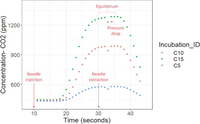
Figure 17: Optimal measuring time for an individual soil sample incubated at three different temperatures. This graph shows the injection and extraction time of the needle, the equilibrium of CO₂ for 5 s, and the pressure drop associated with the selected time frame. Incubation_ID shows block position (C) and vial positions (5, 10, and 15). Please click here to view a larger version of this figure.

Testing the full protocol
To evaluate the functionality and reproducibility of the protocol, we incubated two different samples, each with four technical replicates, across the 22 discrete temperatures ranging from 4 °C to 60 °C. These soil samples were chosen to demonstrate the type of data generated with this setup and its performance. Specific sample characteristics can be found in Supplementary Table 2. The temperature gradient block reliably captured the soil respiration rates of the different soil samples at each temperature point, allowing us to visualize the temperature response curve. Additionally, the resulting temperature response curves for all replicates were nearly identical, as reflected by the small standard deviation around the mean respiration rates across all temperatures (Figure 18). These results demonstrate high reproducibility and confirm the precision of the protocol.

Figure 18: Representative SOM decomposition rates (Rs) for two soils, each measured with four technical replicates incubated across the full temperature gradient. Points represent the mean of respiration rates at each temperature, and error bars indicate the standard deviation among technical replicates. Please click here to view a larger version of this figure.

A second test was performed to demonstrate the scientific applicability of the protocol. We measured soil respiration rates across the full temperature gradient and fitted the data using the Arrhenius or MMRT model (Figure 19). These soil samples were chosen to demonstrate the system performance for contrasting temperature response curves (sample characteristics are provided in Supplementary Table 2). Results show that the data collected with the temperature gradient block can be further analyzed by testing different theories about the temperature sensitivity of SOM decomposition rates. However, challenges arise when working with fresh soil in any experiment. During the 10 days pre-incubation period, we observed fungal communities growing inside some of the vials in soil samples beyond the set of representative samples. Despite our efforts to carefully remove the fungal communities without disturbing the soil, this growth impacted the results of some samples (Figure 20). Consequently, we decided to discard the affected samples by removing the entire sample, not just the individual vials impacted by fungal growth.

Figure 19: Representative results and respiration rates (Rs) of four different soil samples incubated in the temperature gradient block. The red line represents the (A,B) Arrhenius fit, and the blue line represents the (C,D) MMRT fit. Please click here to view a larger version of this figure.

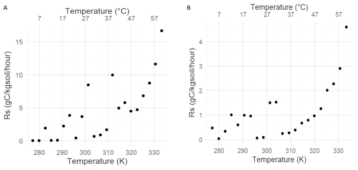
Figure 20: Respiration rate patterns for some samples affected by fungal growth. These results are examples of (A,B) two contaminated samples that were excluded from further analysis. Please click here to view a larger version of this figure.

Supplementary Figure 1: Basic NO/NC circuit. "C" may also be labeled as "COM" for Common. Please click here to download this File.

Supplementary Figure 2: Cooling system control panel. Please click here to download this File.

Supplementary Figure 3: System switch and light indicator. (A) Temperature gradient block control system switch; and (B) green light indicating the sensors and heating system are ON. Please click here to download this File.

Supplementary Figure 4: Temperature gradient block heater control in the online interface. Please click here to download this File.

Supplementary Figure 5: Diagnostic section of the gas analyzer. Everything is green means that the instrument is ready for measurements. Please click here to download this File.

Supplementary Figure 6: Water holding capacity of soils incubated at different temperatures, measurements recorded after 3.5 h of block incubation. Please click here to download this File.

Supplementary File 1: Detailed wiring instructions. Please click here to download this File.

Supplementary Table 1: List of materials with the required quantity. Please click here to download this File.

Supplementary Table 2: Characteristics of soil samples used for the moisture loss test and full protocol. These samples were chosen to demonstrate the functionality of the protocol. Texture classification follows the USDA system, with coarse, clay, silt, and sand expressed as percentages. OC refers to organic carbon content (g C·kg^-1 soil), pH was measured in water, and CaCO₃ represents calcium carbonate content (g·kg^-1 soil). Please click here to download this File.

Discussion

Using a temperature gradient block for measuring the short-term temperature response of SOM decomposition rates presents challenges, especially in detecting respiration rates at low temperatures. Low temperatures can directly inhibit the catalytic activities of intracellular and extracellular enzymes^46,47. Therefore, the incubation time must be long enough to ensure that the low respiration rates at the low end of the temperature range allow for a sufficient build-up of CO₂ in the glass vials to fall within the detection range of the gas analyzer. In this experimental setup, the lowest temperature was 4.1 °C; these samples were the first ones to be loaded into the block and last to be analyzed, giving extra incubation time. The ~3.5 h of block incubation time were found to be sufficient to yield detectable changes in CO₂ concentration in the samples. This incubation length is likely to depend on soil type and particularly organic matter content. For example, it may be that sandy soils with low organic matter content may require longer incubation times than carbon-rich soils. However, in the tests here, the incubation time of 3.5 h was found to be generally sufficient for most soil types and organic content levels.

In addition to optimizing incubation time for CO₂ detection at low temperatures, it is equally important to minimize moisture loss at the higher end of the temperature gradient. Soil moisture plays a crucial role in transportation, diffusion, and dissolution of substrates to microbial communities⁴⁸. For instance, soil moisture can limit respiration rates by restricting substrate diffusion at low moisture levels and reducing oxygen availability at high moisture levels^45,49. Thus, minimizing moisture loss at high temperatures is relevant to prevent moisture from limiting microbial access to substrates. Although the vials in this protocol were completely sealed, water condensed on the caps and inner walls of the vials. This condensation was considered as moisture lost from the soil. Thus, we reduced the incubation time from 4 h, as in Robinson et al. 2017⁴¹, to 3.5 h. While it was not possible to maintain completely constant moisture levels across all temperature treatments, soils were kept at optimal moisture levels during the 3.5 h incubation period. Even at high temperatures, the WHC of the soil remained above 50%, ensuring that water availability did not limit microbial access to substrates^44,45.

Another important consideration is the temperature range of the incubation. While the cooling system can reach temperatures as low as -30 °C and the heating system up to 320 °C, the insulation material has a temperature tolerance of -183 °C to 148 °C. The glass vials used in this setup can withstand 500 °C. Although these ranges are wide, incubating samples above 100 °C possesses a safety concern for the operator. To prevent overheating, a thermal resistor was added, ensuring the heating system automatically shuts down if the aluminum block reaches 90 °C. The inclusion of this thermal resistor is crucial due to the observed initialization overshoot (Figure 13A). If the temperature during the initialization overshoots above 90 °C the system will be disabled. Given these limitations, we recommend operating this setup to a maximum temperature of 60 °C for safe and reliable performance. Additional testing is required for incubating soil samples below 0 °C to ensure reliable CO₂ detection, as condensation and associated moisture variability may affect measurements at subzero temperatures. For this protocol, we chose a lower temperature limit of 4 °C, at which no condensation was observed. If the system is used at wider temperature ranges, we recommend implementing additional thermal safety guidelines.

Another potential constraint of this method is that the relatively short incubation period does not allow microbial communities to adapt to changes in temperature. The temperature response of soils exposed to sustained warming has been the focus of many studies, particularly with the aim of testing microbial adaptation theories^{27,43,47,50,51}. Microbial adaptation has been proposed to explain the diminishing effect over time of experimental warming on soil respiration rates⁴⁷. However, the methodology presented here was developed to measure the short-term temperature response of SOM decomposition rates. While microbial adaptation is unlikely to occur in short periods of time⁴⁷, a recent study used a similar methodology to quantify the rate of microbial adaptation by incubating soils from a geothermal gradient. In this study, MMRT was fitted to estimate key parameters, including the temperature optima and inflection points. By comparing these parameters across soils from the geothermal gradient, the findings show that the rate of microbial adaptation is significantly lower than the rate of warming⁵². This study highlights the importance of understanding the whole temperature response curve, particularly capturing the temperature optimum and inflection points of biological soil processes (Figure 19C,D). In light of these findings, we recommend sampling microbial communities at multiple temperature points during block incubation to assess how microbial community composition and functions correlate with respiration rates and temperature sensitivity parameters.

The temperature gradient block outlined in this paper offers significant advantages over traditional methodologies. One major benefit is that it enables researchers to measure SOM decomposition rates efficiently and accurately at 22 discrete temperatures with small amounts of soil. This represents a methodological improvement compared to incubating soil samples at a few discrete temperatures, which compels researchers to apply the Q₁₀ temperature coefficient - a method that many studies have challenged^12,13,15. Another significant benefit is that this setup collects data that clearly captures the shape and steepness of the temperature response curve. The number of discrete temperature treatments along a wide temperature gradient allows us to identify the inflection point temperature and optimum of biological processes, allowing comparisons between treatments. The examples presented in this manuscript show two distinct patterns (Figure 19A,B vs. Figure 19C,D), which researchers can further analyze using different temperature sensitivity theories. Some examples support the Arrhenius theory, where reaction rates increase exponentially with temperature (Figure 19A,B). In contrast, other examples align with the MMRT theory, showing a unimodal response with a clear temperature optimum (Figure 19C,D). These two different patterns indicate that the presented temperature block incubation protocol is capable of reproducing both types of response curves, which can be used to test theories of the temperature sensitivity of SOM decomposition rates, thereby deepening our understanding of thermodynamics, biology, and chemistry.

Materials

List of materials used in this article

Name	Company	Catalog Number	Comments
630 mA glass fuse	RS	563-637	https://uk.rs-online.com/web /p/cartridge-fuses/0563637?gb=s
Adhesive sealant	Innotec	01.2451.0000	https://www.innotec.nl /producten/adheseal
Aluminium block	metaalketen	96082150.1	https://www.metaalketen .com/aluminium/
Aluminum tape	Manutan	A159435	https://www.manutan.nl/nl/mnl/aluminiumtape -met-schutlaag-50565-50-m-x-50-mm-tesa -a159435?shoppingab=true&gad_source= 1&gclid=CjwKCAjw74e1Bh BnEiwAbqOAjE5Tw3-r3xiW 9FWALDZMlVUWpqJpQQ R_zwwXR8_R6Sb1Ce_8v x96jxoCtx4QAvD_BwE
Black wire	RS	361-787	https://nl.rs-online.com/web /p/hook-up-wire/0361787
Blue wire	RS	724-4392	https://nl.rs-online.com/web /p/hook-up-wire/7244392
Brown wire	RS	724-4395	https://nl.rs-online.com/web /p/hook-up-wire/7244395
Cable gland	RS	807-9786	https://nl.rs-online.com/web/p /cable-glands/8079786?cm_ mmc=NL-PLA-DS3A-_-goog le-_-CSS_NL_EN_Cables_% 26_Wires_Whoop-_-(NL:Who op!)+Cable+Glands-_-807978 6&matchtype=&aud-8271861 83926:pla-339598489905&gcli d=Cj0KCQiAw8OeBhCeARIsA GxWtUyscrqjF3FwA6j2jqUyeg_ s70tOXBRuYRF90pwubv3Po8v sbZSJhV4aAq84EALw_wcB&gc lsrc=aw.ds
Circular saw	Ryobitools	RWSL1801M	https://nl.ryobitools.eu/elektrisch-g ereedschap/zaagmachines/cirkelz agen/rwsl1801/rwsl1801m/?gad_so urce=1&gclid=Cj0KCQjw2ou2BhCC ARIsANAwM2Easx4PAZzvVYvFFUD ZKemTdqNDXsde_NDPSB8FAlGu7 8Hzy2j3TuoaAhTjEALw_wcB
Closures	Kramp	HS491976	https://www.kramp.com/shop-nl/nl/p /verstelbare-haakvergrendeling-118- 128-typ.3--HS491976
Cooler and natural cooling agent	Dijkstra Vereenigde	L035004186	https://www.laboratorium-apparatuur .nl/ika-rc2-green-basic-koelthermo staat-30-c-bad-volume-4-liter-l035004186
DIN Rail	RS	648-5722	https://nl.rs-online.com/web/p/din-ra ils/6485722?cm_mmc=NL-PLA-DS 3A-_-google-_-CSS_NL_NL_Pmax _Test-_--_-6485722&matchtype=&&g ad_source=1&gclid=CjwKCAjw8f u1BhBsEiwAwDrsjOqGDs92gjrJHkp SsYmOiS0OK6tC9U_fMHEhlmvu7r SbNp8VnmuDERoCC0UQAvD_ BwE&gclsrc=aw.ds
Dual bridges	RS	803-7530	https://nl.rs-online.com/web/p/din-rail -terminal-accessories/8037530?sear chId=11c9702f-3312-4bb0-a826-e9d 50bd91ee1&gb=s
Ethernet cable	RS	657-2090	https://nl.rs-online.com/web/p/ ethernet-cable/6572090
Face mask	KN95	NA	https://www.bol.com/nl/nl/p/kn95- disposable-face-mask-ffp2-x-1-mask s-kn95-wegwerp-gezichtsmasker-ffp 2-x-1mondkapjes/930000000131403 0/?Referrer=NLGOOFS&utm_source =google&utm_medium=free_shopping
Female connector	qosina	17642	https://www.qosina.com/female- to-female-luer-lock-connector-17642
Filter 0.45 µm	Whatman	10462650	https://us.vwr.com/store/product/1394 3097/whatmantm-puradisc-aqua-30-m m-syringe-filter-0-45-m-whatman- products-cytiva
Flexible insulation (hose)	Celsis	4600000198	https://www.celsisbv.nl/k-flex-plaati solatie-op-rol-st-10e-1x10mtr-10mm .-bl-s3-d0/4600000198?gad_source =1&gclid=Cj0KCQjw8MG1BhCoARI sAHxSiQknvLK3RcqgqXwR1Ma7V PznSz8IasKUGvLo0SySzLiff2o_kK Vjip0aAtATEALw_wcB
Flexible tube	Avantor	MFLX06491-14	https://www.avantorsciences.com /de/en/product/38670173/bev-a- line-v-transfer-pump-tubing
Flow reduction kit	LICOR	7800-113	https://www.licor.com/support /Trace-Gas-Analyzers/topics/re duced-flow-rate-kit-7800-113.html
Fuse holder terminal	Elektramat	401144228	https://nl.mouser.com/ProductD etail/Phoenix-Contact/3270200? qs=zdVlZaK%252BC241RFTPi Xj4mA%3D%3D&mgh=1&utm_i d=20328035028&gad_source=1 &gclid=CjwKCAjw8fu1BhBsEiwA wDrsjBg9elAMYS9bWJ1Bd086J 7fGBWvcRWZ51okdr2qJgOlOTd BdrUZ_rBoCvuUQAvD_BwE
Gas analyzer	LICOR	LI-7815	https://www.licor.com/env/ products/trace-gas/LI-7815
Glass vials with caps 60 mL	Cole-Parmer	GZ-99535-25	https://www.coleparmer.com/i/ cole-parmer-precleaned-epa- vials-clear-glass-60-ml-72-cs/9953525
Green/yellow wire	RS	721-0636	https://nl.rs-online.com/web /p/hook-up-wire/7210636
Handles	RS	456-539	https://nl.rs-online.com/web/p/ drawer-handles-cabinet-han dles/0456539
Heating Rods	RS	860-6984	https://www.reichelt.com/nl/nl/shop /product/verwarmingspatroon_hotr od_20_0x250_mm_1250_w_230_ v_-317248?PROVID=2809&gad_s ource=1&gad_campaignid=22415 164764&gbraid=0AAAAADwnxtY mY6n2NPja4HF_ftn_kJY-U&gcli d=CjwKCAjwiNXFBhBKEiwAPSa PCaYMjfVMKQazvkQk_deE2koc XA9SZ_ltbPIefniuRsmzBwN_oQ rfQhoCegUQAvD_BwE
Hinges	RS	448-1497	https://benl.rs-online.com/ web/p/hinges/4481497
Hose	Wildkamp	750568	https://www.slangenboer.nl/wat erslang-cristal-al-961?channabl e=41cdee736b7500534230313 0353131333924&bg_source=ga &bg_campaign=21584331548& bg_kw=pla-293946777986-mi-1 09646330-pi-SB01051139-ppi- 293946777986&bg_source_id= 709628610149&gad_source=1 &gad_campaignid=215843315 48&gbraid=0AAAAADegGXwz 91MJFzGxBRxjCSRew10eG& gclid=CjwKCAjwiNXFBhBKEiw APSaPCZNCdBEfvnV2pYYPeV SQaiG_UKP0q_eknv0lC_N_0Y WIIZQvze8TEhoCzPUQAvD_BwE
Hose barb	Wildkamp	11000357	https://www.wildkamp.nl/pro duct/slangtule-rvs-316l-lost-w ax-buitendraad-x-slangtule-bs p-x-10-0-mm/11000357
Injection needle	Merkala	303262	https://www.merkala.nl/bd-mic rolance-injectienaalden-18g-ro ze-1-2x40mm-100-stuks.html? gclid=CjwKCAjw_Na1BhAlEiw AM-dm7DrC9mGkmpNN8krYe CmkvpEeSv4CuH3I2Px71KJxY YSm-vjVu2LclRoCwuwQAvD_BwE
Injection tube gas analizer 1/4"	VWR	MFLX06491-12	https://us.vwr.com/store/pr oduct/39537334/bev-a-line- v-transfer-pump-tubing
Insulation material	Technische Unie	3603842	https://www.technischeunie. nl/product/prd1899911190
Knee couplings	Kramp	MMI9006K	https://www.kramp.com/shop-nl/ nl/p/haakse-koppeling-instelbaa r-bu-bu-3-8-bsp--MMI9006K
Large diameter tube 3/8"	Avantor	39213360	https://www.avantorsciences.co m/us/en/product/39213360/mast erflex-transfer-tubing-flexible- vinyl-avantor
M6 Screws, Hex	RS	281-120	https://nl.rs-online.com/web/p/so cket-screws/0281120?srsltid=Afm BOorVGq-ZyA2yrJG1kU7SHGiZ EblaRz0nDmX7MwhzIRjcc6P4YIYE
Main junction box	RS	Check Dia.	https://nl.rs-online.com/w eb/p/general-purpose-enclo sures/2896320?gb=s
Male connector	qosina	12090	https://www.qosina.com/male- to-male-luer-lock-connector-12090
Male Luer	Walternedical	BPC04M	https://www.waltersmedical.co. uk/product/nibp-connector-male-luer-slip/
MCB - Siemens SENTRON	RS	3RF2320-1AA02	https://nl.rs-online.com/we b/p/mcbs/2383188?gb=s
PE/DND feedtrhough	RS	687-9411	https://uk.rs-online.com/we b/p/din-rail-terminal-blocks/ 6879411?searchId=c9a9c1 b1-3def-40d0-8b14-b792f8269615&gb=s
Power Indication LED	RS	909-2437	https://uk.rs-online.com/ web/p/pilot-lights/9092437?gb=s
Power supply	Antratek	X-2902992	https://nl.rs-online.com/web/ p/din-rail-power-supplies/054 0731?srsltid=AfmBOoqMPIO Av7bZd1Qu_Acy3KMFR0-x OD_Hkw3NeQCYyzKJLzEGXzxQ
Quintople conductor bridges	RS	803-6713	https://uk.rs-online.com/web /p/din-rail-terminal-blocks/80 36713?searchId=7de6627a- 3634-42ed-a600-2e3ce8974fe7&gb=s
Red wire	RS	361-822	https://nl.rs-online.com/web /p/hook-up-wire/0361822
Ring Terminal 2.5 mm²	RS	534-569	https://uk.rs-online.com/ web/p/ring-terminals/0534569
Sensors	Antratek	X-DTS-S3C	https://www.antratek.nl/dig ital-temperature-sensor-1m-cable
Septa Red Butyl	HomeGreen	A255	https://www.homegreen.nl/la b-benodigdheden/septa-rood -butyl-20-mm?srsltid=AfmBO ooStonU5v9Q9j7i_RgQMJ9F m6ZVbPbIRU0cD1_47-BEVmb1r5I5
Single conductor feedthrough	Elektramat	401167865	https://www.elektramat.nl/ catalogsearch/result/?q=401167865
Single-phase power cable	RS	626-6694	https://nl.rs-online.com/w eb/p/power-cords/6266694?gb=s
Single-phase wire	RS	775-6123	https://uk.rs-online.com/web /p/power-cable/7756123?gb=s
Small junction box	RS	498-5387	https://nl.rs-online.com/web/p /general-purpose-enclosures/4985387
Solid State Relay	RS	467-4762	https://nl.rs-online.com/web/p /solid-state-relays/4674762
Spiral drill	Ericks	10471300	https://shop.eriks.nl/nl/gereed schappen-verspanende-geree dschappen-boren-hss-en-hsse -boren-cilindrische-schacht/spir aalboor-din340-hsse-geslepen- type-ti-5-80mm-12592599/?srslt id=AfmBOoopMLgX1mtyuUxkU KU7jW4fYY1bY5wSTvSGQUkO zTc6E2wdxUZQ
Stainless steel housing and lid	247 Tailore steel		https://247tailorsteel.com/nl/?ut m_term=24%207%20steel&utm _campaign=B+-+NL+-+247tailo rsteel+-+NL+-+Doelvertonings percentage+%3E+Conv.+Waa rde+met+Doel-ROAS&utm_so urce=adwords&utm_medium= ppc&hsa_acc=2007690635&h sa_cam=783787418&hsa_grp =118504886580&hsa_ad=67 1662182959&hsa_src=g&hsa _tgt=kwd-374862287021&hs a_kw=24%207%20steel&hsa _mt=p&hsa_net=adwords&hsa _ver=3&gad_source=1&gclid= Cj0KCQjw8MG1BhCoARIsAHx SiQnhmktBk_3c_wobSJobrTVp4 _nqiW26Zt7XzSkHdK-htW8medy NCcQaAjbrEALw_wcB
Switch 2-way	RS	746-9336	https://nl.rs-online.com/web/p /cam-switch-handles/7469336
Terminal bridge	Elektramat	401043503	https://www.elektramat.nl/phoenix-c ontact-doorverbindingsbrug-voor-rijg klem-2-polig-5-2-mm-rood-fbs-2-5/?c hannable=0141ac6964003330383936 ec&utm_source=google-surfaces&utm _medium=organic&bg_source=ga&bg_ campaign=19011971421&bg_kw=-mi-9 214030-pi-401043503-ppi-&bg_source _id=&gad_source=1&gclid=CjwKCAjw 8fu1BhBsEiwAwDrsjE2kRcDZUHPupfy haLoTzWLqM9v8HKaiI67st4UOmUXIN 9OaI25ALRoCvmUQAvD_BwE
Thermostat DAQ	Antratek	X-300-I	Temperaturüberwachung & Thermostat (+X-DTS-S3C) von ControlByWeb (antratek.nl)
Universal Milling Machine	Mach4Metal	MACH-ID 7580	https://mach4metal.com/en /milling-machines/cnc/fehlm ann-picomax-p54-2
Wago 3 conductor feedthrough	RS	803-6713	https://nl.rs-online.com/web/ p/din-rail-terminal-blocks/80 36713?cm_mmc=NL-PLA-D S3A-_-google-_-CSS_NL_N L_Pmax_0525-_--_-803671 3&matchtype=&&gclsrc=aw.d s&gad_source=1&gad_campa ignid=22555696009&gbraid=0 AAAAADkeWNNXeREaDmJ5n yYqYMqp-c7A6&gclid=CjwKCAj wtfvEBhAmEiwA-DsKjilXxL8uO 4Jo6XyDesHGaQkoz6Ggi4ATI6 FUInWV9TxmIX519DGIZBoCh9 YQAvD_BwE
Wago connector	RS	883-7557	https://uk.rs-online.com/ web/p/standard-terminal-b locks/8837557?gb=s
Wire end sleeves (100 pc)	Elektramat	401173609	https://www.elektramat.nl/solar -adereindhuls-geisoleerd-2-5mm 2-hulslengte-8mm-blauw-per-100 -stuks-1505145/?channable=014 1ac696400343034a4&utm_source =google-surfaces&utm_medium =organic&bg_source=ga&bg_c ampaign=17673967332&bg_kw= -mi-9214030-pi-401173609-ppi-&bg _source_id=&gad_source=1&gclid= CjwKCAjw8fu1BhBsEiwAwDrsjNms VYTNZ5TuXEHtsF34hcY-T5kLFnhi zir1fUsR3UYcG9bxmugqJRoCp_Y QAvD_BwE

References

- Foote, E. Circumstances affecting the heat of the Sun's rays. Am J Sci Arts. , 382-383 (1856).
- Jackson, R. Eunice Foote, John Tyndall and a question of priority. Notes Rec. 74, 105-118 (2020).
- Friedlingstein, P., et al. Global carbon budget 2024. Earth Syst Sci Data. 17, 67(2025).
- Bond-Lamberty, B., Thomson, A. Temperature-associated increases in the global soil respiration record. Nature. 464, 579-582 (1960).
- Raich, J. W., Potter, C. S. Global patterns of carbon dioxide emissions from soils. Glob Biogeochem Cycles. 9, 23-36 (1995).
- Davidson, E. A., Janssens, I. A. Temperature sensitivity of soil carbon decomposition and feedbacks to climate change. Nature. 440, 165-173 (2006).
- Conant, R. T., et al. Temperature and soil organic matter decomposition rates-synthesis of current knowledge and a way forward. Glob Chang Biol. 17, 3392-3404 (2011).
- Todd-Brown, K. E. O., et al. Causes of variation in soil carbon simulations from CMIP5 Earth system models and comparison with observations. Biogeosciences. 10, 1717-1736 (2013).
- Crowther, T. W., et al. Quantifying global soil carbon losses in response to warming. Nature. 540, 104-108 (2016).
- Wieder, W. R., et al. Carbon cycle confidence and uncertainty: Exploring variation among soil biogeochemical models. Glob Chang Biol. 24, 1563-1579 (2018).
- van Gestel, N., et al. Predicting soil carbon loss with warming. Nature. 554, E4-E5 (2018).
- Liáng, L. L., Kirschbaum, M. U. F., Arcus, V. L., Schipper, L. A. The carbon-quality temperature hypothesis: Fact or artefact. Glob Chang Biol. 29 (4), 935-942 (2022).
- Sierra, C. A. Temperature sensitivity of organic matter decomposition in the Arrhenius equation: Some theoretical considerations. Biogeochemistry. 108, 1-15 (2012).
- Lloyd, J., Taylor, J. A. On the temperature dependence of soil respiration. Funct Ecol. 8, 315(1994).
- Moinet, G. Y. K., Morán-Rivera, K., Moinet, A., Wadoux, A. M. J. C. Large underestimations of warming-induced soil carbon emissions from oversimplistic Q10 indicator. Soil Biol Biochem. 207, 109839(2025).
- Arrhenius, S. On the influence of carbonic acid in the air upon the temperature of the ground. Philos Mag J Sci. 41, 237-276 (1896).
- Alster, C. J., Koyama, A., Johnson, N. G., Wallenstein, M. D., von Fischer, J. C. Temperature sensitivity of soil microbial communities: An application of macromolecular rate theory to microbial respiration. J Geophys Res Biogeosci. 121, 1420-1433 (2016).
- Thomas, T. M., Scopes, R. K. The effects of temperature on the kinetics and stability of mesophilic and thermophilic 3-phosphoglycerate kinases. Biochem J. 330, 1087-1095 (1998).
- Daniel, R. M., Danson, M. J. A new understanding of how temperature affects the catalytic activity of enzymes. Trends Biochem Sci. 35, 584-591 (2010).
- Ruller, R., Deliberto, L., Ferreira, T. L., Ward, R. J. Thermostable variants of the recombinant xylanase A from Bacillus subtilis produced by directed evolution show reduced heat capacity changes. Proteins. 70, 1280-1293 (2008).
- Numa, K. B., Robinson, J. M., Arcus, V. L., Schipper, L. A. Separating the temperature response of soil respiration derived from soil organic matter and added labile carbon compounds. Geoderma. 400, 115128(2021).
- Prentice, E. J., et al. The inflection point hypothesis: The relationship between the temperature dependence of enzyme-catalyzed reaction rates and microbial growth rates. Biochemistry. 59, 3562-3569 (2020).
- Howard, P. J. A., Howard, D. M. Respiration of decomposing litter in relation to temperature and moisture: Microbial decomposition of tree and shrub leaf litter 2. Oikos. 33, 457(1979).
- DeLong, J. P., et al. The combined effects of reactant kinetics and enzyme stability explain the temperature dependence of metabolic rates. Ecol Evol. 7, 3940-3950 (2017).
- Alster, C. J., von Fischer, J. C., Allison, S. D., Treseder, K. K. Embracing a new paradigm for temperature sensitivity of soil microbes. Glob Chang Biol. 26, 3221-3229 (2020).
- Hobbs, J. K., et al. Change in heat capacity for enzyme catalysis determines temperature dependence of enzyme catalyzed rates. ACS Chem Biol. 8, 2388-2393 (2013).
- Moinet, G. Y. K., et al. Soil microbial sensitivity to temperature remains unchanged despite community compositional shifts along geothermal gradients. Glob Chang Biol. 27 (23), 6217-6231 (2021).
- Schipper, L. A., Hobbs, J. K., Rutledge, S., Arcus, V. L. Thermodynamic theory explains the temperature optima of soil microbial processes and high Q10 values at low temperatures. Glob Chang Biol. 20, 3578-3586 (2014).
- Kirschbaum, M. U. F. Soil respiration under prolonged soil warming: Are rate reductions caused by acclimation or substrate loss. Glob Chang Biol. 10, 1870-1877 (2004).
- Kirschbaum, M. U. F. The temperature dependence of organic-matter decomposition-still a topic of debate. Soil Biol Biochem. 38, 2510-2518 (2006).
- Moinet, G. Y. K., et al. The temperature sensitivity of soil organic matter decomposition is constrained by microbial access to substrates. Soil Biol Biochem. 116, 333-339 (2018).
- Moinet, G. Y. K., et al. Temperature sensitivity of decomposition decreases with increasing soil organic matter stability. Sci Total Environ. 704, 135460(2020).
- Moinet, G. Y. K., Millard, P. Temperature sensitivity of decomposition: Discrepancy between field and laboratory estimates is not due to sieving the soil. Geoderma. 374, 0-3 (2020).
- Fang, C., Smith, P., Moncrieff, J. B., Smith, J. U. Similar response of labile and resistant soil organic matter pools to changes in temperature. Nature. 433, 57-59 (2005).
- Knorr, W., Prentice, I. C., House, J. I., Holland, E. A. Long-term sensitivity of soil carbon turnover to warming. Nature. 433, 298-301 (2005).
- Walker, T. W. N., et al. Microbial temperature sensitivity and biomass change explain soil carbon loss with warming. Nat Clim Chang. 8, 885-889 (2018).
- Wankhede, M., et al. Does soil organic carbon quality or quantity govern relative temperature sensitivity in soil aggregates. Biogeochemistry. 148, 191-206 (2020).
- Sáez-Sandino, T., et al. The soil microbiome governs the response of microbial respiration to warming across the globe. Nat Clim Chang. 13, 1382-1387 (2023).
- Vaughn, L. J. S., Torn, M. S. 14C evidence that millennial and fast-cycling soil carbon are equally sensitive to warming. Nat Clim Chang. 9, 467-471 (2019).
- Liu, Y., et al. Temperature sensitivity of soil microbial respiration in soils with lower substrate availability is enhanced more by labile carbon input. Soil Biol Biochem. 154, 108148(2021).
- Robinson, J. M., et al. Rapid laboratory measurement of the temperature dependence of soil respiration and application to changes in three diverse soils through the year. Biogeochemistry. 133, 101-112 (2017).
- Thomas, W. H., Scotten, H. L., Bradshaw, J. S. Thermal gradient incubators for small aquatic organisms on JSTOR. Limnol Oceanogr. 357, 357-360 (1963).
- Alster, C. J., Robinson, J. M., Arcus, V. L., Schipper, L. A. Assessing thermal acclimation of soil microbial respiration using macromolecular rate theory. Biogeochemistry. 158, 131-141 (2022).
- Sierra, C. A., Trumbore, S. E., Davidson, E. A., Vicca, S., Janssens, I. Sensitivity of decomposition rates of soil organic matter with respect to simultaneous changes in temperature and moisture. J Adv Model Earth Syst. 7, 335-356 (2015).
- Davidson, E. A., Samanta, S., Caramori, S. S., Savage, K. The dual Arrhenius and Michaelis-Menten kinetics model for decomposition of soil organic matter at hourly to seasonal time scales. Glob Chang Biol. 18, 371-384 (2012).
- Schuur, E. A. G., et al. Climate change and the permafrost carbon feedback. Nature. 520, 171-179 (2015).
- Bradford, M. A. Thermal adaptation of decomposer communities in warming soils. Front Microbiol. 4, 333(2013).
- Tecon, R., Or, D. Biophysical processes supporting the diversity of microbial life in soil. FEMS Microbiol Rev. 41, 599-623 (2017).
- Evans, S. E., Allison, S. D., Hawkes, C. V. Microbes, memory and moisture: Predicting microbial moisture responses and their impact on carbon cycling. Funct Ecol. 36, 1430-1441 (2022).
- Allison, S. D., Wallenstein, M. D., Bradford, M. A. Soil-carbon response to warming dependent on microbial physiology. Nat Geosci. 3, 336-340 (2010).
- Elias, M., Wieczorek, G., Rosenne, S., Tawfik, D. S. The universality of enzymatic rate-temperature dependency. Trends Biochem Sci. 39, 1-7 (2014).
- Alster, C. J., et al. Quantifying thermal adaptation of soil microbial respiration. Nat Commun. 14, 1-25 (2023).
Reprints and Permissions