A Data-Driven Framework for Financial Risk Prediction and Control in the Digital Economy

Summary

This research proposes Financial Risk, a data-driven framework designed to improve financial risk prediction and control in the digital economy using distributed learning, dynamic contagion modeling, and interpretability mechanisms.

Abstract

In the era of digital economy, financial management is shifting toward data-driven decision-making. The three most important challenges are: (a) distributed data privacy constraints, (b) rapid contagion of financial risks across interconnected enterprises, and (c) transparent decision logic for multiple stakeholders. Financial Risk tackles these challenges with a framework that includes Joint Reinforcement Learning (JRL) for distributed financial decision optimization, an Adaptive Graph Neural Network (AGNN) for modeling real-time contagion effects, and a dual-channel interpretation layer to enhance transparency. Experiments were conducted using quarterly financial data from 2018 to 2023 of 300 Chinese A-share listed companies, as well as a simulated distributed dataset. The key findings indicate that JRL achieved a cumulative revenue of 60.8 billion yuan (with a privacy score of 0.92), while the AUC of AGNN reached 0.89 and stabilized errors within two hours after policy shocks. The performance of the interpretation layer has reached 85% accuracy at an average of 2.8 key features. All these findings demonstrate that the Financial Risk framework balances privacy, efficiency, risk control, and interpretability, and offers a practical paradigm for financial risk management in the digital economy.

Introduction

In the digital economy era, corporate financial management will shift from experience-based practices to data-driven paradigms¹. Real-time transactions, IoT sensors, and cloud-based enterprise systems generate multidimensional financial data in a nonstop manner, opening up new vistas for precision forecasting, smart financing, and dynamic asset allocation². Still, financial data is disseminated across subsidiaries, supply chain partners, financial institutions, and regulators, and the increasingly strict legal requirements regarding data security and PIPL make centralized processing difficult. Under these circumstances, the traditional paradigm of "data migration to cloud centralized modeling unified decision-making" is fundamentally faced with a dilemma: sacrificing privacy for efficiency or maintaining data silos at the cost of suboptimal outcomes³.

At the same time, the speed and intensity of financial risk contagion are growing⁴. Macroeconomic fluctuation, geopolitical tension, and unexpected "black swan" events can cascade quickly along supply chains, collateral chains, and capital flows, leading to systemic risk in minutes⁵. Conventional tools, such as static financial statements and credit ratings, are often insufficient for capturing these fast-evolving dynamics. To address this limitation, researchers have explored advanced computational methods, including reinforcement learning for optimization of financial decisions, federated learning for distributed collaboration, and graph neural networks for modeling complex inter-firm dependencies⁶. These approaches have achieved initial success in improving financial forecasting, credit risk control, and contagion modeling; however, most of them assume access to centralized or global data, thus limiting practical applicability in distributed and privacy-constrained contexts⁷.

Another important challenge is that of interpretability. Methods such as SHAP-based feature attribution and decision rule extraction are only partial explanations, and they generally cannot meet the requirements of various stakeholders like CFOs, auditors, and regulators, who require the decision processes to be transparent, auditable, and semantically accessible⁸. Without interpretability, even highly accurate models struggle to gain adoption in real financial decision-making environments⁹. Deep reinforcement learning methods such as DDPG¹ provided foundational advances that underpin modern financial decision-systems¹⁰.

The proposed framework assumes, from the application perspective, an enterprise network wherein the financial data is spread out among subsidiaries, supply-chain partners, financial institutions, or regulatory nodes, where raw-data pooling cannot be done owing to privacy or jurisdictional constraints¹¹. The approach works well in a scenario when each enterprise node supplies time-series financial indicators-usually ranging from 50 to 120 features that cover capital structure, liquidity, profitability, and credit events-across numerous reporting periods¹². The framework can be deployed on standard GPU-enabled or high-performance CPU environments and supports a number of privacy law contexts, such as GDPR, CCPA, and China's PIPL, by exchanging encrypted model parameters rather than sensitive financial records^13,14. Typical system requirements include moderate communication frequency between nodes and stable network topology over time. A known limitation is reduced accuracy under extremely sparse or highly volatile enterprise networks, wherein rapid structural shifts prevent the graph model from learning steady inter-firm dependencies. In such cases, frequent retraining or shorter time windows may be required to maintain predictive stability¹⁵.

Against this backdrop, the present study proposes Financial Risk, a data-driven framework that integrates Joint Reinforcement Learning (JLR) for distributed optimization¹⁶, an adaptive graph neural network for real-time contagion modeling¹⁷, and a dual-channel interpretation layer for stakeholder-oriented transparency¹⁸. By simultaneously addressing privacy, efficiency, risk control, and interpretability, this framework provides a new paradigm for financial management in the digital economy.

Protocol

This protocol describes the steps to construct the Financial Risk framework for financial risk prediction and control in the digital economy and to reproduce the corresponding validation experiments. The protocol covers mathematical model formalization, framework module construction, workflow integration, dataset preparation, baseline setup, and evaluation metric definition, enabling reproducibility by researchers in the field. The Table of Materials summarizes all software, libraries/toolkits, hardware resources, and datasets required to reproduce this protocol, while Figure 1 provides the overall workflow for transparent financial risk prediction and control.

NOTE: All steps in this protocol are implemented in a Python-based workflow. Local enterprise agents (clients) are executed on separate machines or isolated containers to emulate distributed institutions, while federated aggregation is executed on a central coordinator (server). Model training and inference are implemented using a deep-learning framework (e.g., PyTorch or TensorFlow) with GPU acceleration when available. Graph neural network operations are implemented using a graph learning library (e.g., PyTorch Geometric or DGL). SHAP explanations are generated using the SHAP package. To ensure reproducibility, experiments use fixed random seeds, predefined train/validation/test splits, consistent preprocessing scripts, and logged hyperparameters (learning rate, batch size, communication rounds, and early-stopping criteria).

1. Define the research problem and formalize mathematical models

1. Clarify the three core research objectives: optimize financial decisions under distributed data privacy constraints, capture dynamic inter-enterprise risk contagion, and ensure human-interpretable decision logic for multi-stakeholders.
2. Formalize the distributed financial decision optimization model
   1. Define the decision space for each enterprise: let decisions at time t for enterprise i be , where A_i  includes investment, financing, and dividend strategies.
   2. Set the long-term return maximization target as the optimization objective, expressed as:
      (1)
      where γ is the discount factor, r_i is the instantaneous reward,  the local state, and  the set of inter-enterprise relationships.
      NOTE: This reward formulation encourages each enterprise agent to optimize decision-making based not only on its own financial status but also on the risk propagation effects on connected enterprises. As a result, JRL supports collaborative yet privacy-preserving learning across distributed financial entities.
   3. Impose privacy constraints: specify that the raw data of each enterprise cannot be shared across entities (i.e., data remain local to each enterprise), and mandate parameter sharing instead of data exchange during federated training.
3. Formalize the dynamic risk contagion model
   1. Represent the inter-enterprise network as a dynamic graph:
         (2)
      where V denotes enterprise nodes and E^t denotes time-varying contagion edges.
   2. Define edge weights  to quantify the risk transmission intensity from enterprise i to j at time t.
   3. Describe the evolution of enterprise i's risk state  using a nonlinear dynamic equation:
      
      Where f is a nonlinear activation function and ∈^t a stochastic disturbance.
4. Formalize the interpretability constraint model
   1. Set the explanation accuracy threshold: require the probability of the model output matching the explanation to satisfy
         (4)
      With δ as the acceptance threshold, while conciseness is maintained by limiting the number of explanatory features.
      NOTE: The acceptance threshold is set to δ = 0.85 based on calibration on the validation set. This threshold controls the minimum agreement between the model output and the generated explanation, ensuring explanations remain faithful to the predicted risk probability while avoiding overly long feature lists.
   2. Impose explanation conciseness by limiting the number of key explanatory features to k≤K  (where K is a pre-defined maximum number of interpretable features).

2. Construct the JRL framework

1. Deploy local reinforcement learning networks for each enterprise
   NOTE: This step is performed on each enterprise client (local machine/container). Only model parameters (or parameter updates) are communicated to the server during federated aggregation.
   1. Implement a Deep Deterministic Policy Gradient (DDPG) agent for each enterprise, including an actor-critic structure (policy network for action selection and critic network for value estimation).
      NOTE: Each client initializes the DDPG agent with a fixed random seed, interacts with its local environment to generate  transitions, and stores them in a replay buffer for minibatch updates.
   2. Define the critic network output to evaluate the value of state-decision pairs:
         (5)
2. Define the loss function for the critic network
   1. Calculate the temporal difference error using the target critic network Q_ϕi , and set the loss function as:
         (6)
   2. Optimize the critic network parameters ϕ_i using stochastic gradient descent. In each update step, sample a minibatch of transitions from the replay buffer, compute the TD loss above, backpropagate gradients, and apply an optimizer update (e.g., SGD/Adam). Optionally apply gradient clipping for stability and update the target critic network using a soft-update rate τ.
3. Optimize the policy network parameters
   1. Compute the gradient of the long-term return J(θ_i) with respect to policy parameters θ_i:
         (7)
   2. Update θ_i using the computed gradient to maximize the cumulative return.
4. Implement global parameter aggregation via Federated Averaging (FedAvg)
   1. Collect encrypted policy network parameters (or parameter deltas) from all enterprises at the end of each communication round.
   2. Calculate the global parameter θ_g by weighting each enterprise's parameters by its dataset size |D_i|:
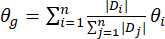         (8)
   3. Distribute the updated global parameter θ_g back to each enterprise to synchronize local networks.
      NOTE: Steps 2.4.1-2.4.3 are performed with a server-client workflow. Clients upload parameters (or deltas) to the central server through an encrypted channel (e.g., TLS). The server performs FedAvg and broadcasts θ_g back to all clients for the next round.
5. Enhance communication efficiency
   1. Apply quantized compression to model parameters to reduce data transmission volume.
   2. Inject differential-privacy noise into each local model update using the Gaussian mechanism. For each round t, noise ∈^t ∼ N(0,σ² I) with σ=0.8 is applied to the gradient vector g:
         (9)
      NOTE: Noise is applied locally on the client immediately before communication to the server to support privacy-preserving training under differential-privacy constraints.
   3. Accept asynchronous updates to accommodate heterogeneous computational abilities across participants.

3. Build the Adaptive Graph Neural Network (AGNN) for risk contagion modeling

1. Calculate attention weights to inform the dynamic adjacency matrix
   1. Compute the attention coefficient  between enterprise i and j at time t using normalized dot-product attention:
         (10)
      NOTE: These attention weights quantify the influence of each neighbor enterprise on the updated risk state, enabling auditors to trace predictions back to specific relational drivers.
   2. Update the edge weight  using  to reflect real-time contagion intensity.
2. Perform temporal message passing
   1. Aggregate neighbor risk states to generate the message vector for enterprise i
         (11)
3. Update the node risk state using a Gated Recurrent Unit (GRU)
   1. Integrate the current state  and message vector  to compute the next-time-step state:
         (12)
4. Extract risk contagion embeddings and optimize the model
   1. Pass the updated state  through a Multilayer Perceptron (MLP) to generate contagion embeddings:
         (13)
   2. Define the cross-entropy loss function to optimize AGNN parameters:
         (14)
   3. Train the AGNN using backpropagation with a minibatch optimizer (e.g., Adam) until convergence. Construct graph snapshots per time step t and generate temporal batches using sliding windows over {G_t}. Minimize L on the training split and monitor the validation loss each epoch. Apply early stopping when the validation loss does not improve for a predefined number of epochs (patience), or stop at a maximum number of epochs.

4. Develop the dual-channel explainability layer

1. Implement the SHAP-based feature importance channel
   1. Calculate the marginal contribution of each feature x_j to the model output using SHAP values:
         (15)
   2. Where ϕ_j is the SHAP value of feature x_j, representing its additive contribution to the prediction.
   3. Rank features by absolute ϕ_j values to identify key drivers of financial risk decisions.
2. Implement the decision tree-based rule extraction channel
   1. Train a lightweight decision tree surrogate model. Use the same input feature matrix X provided to the Financial Risk model and the corresponding model outputs as supervision signals. Specifically, use either (i) the predicted probability  (regression tree) or (ii) discretized risk levels (classification tree) obtained by thresholding  (e.g., Low/Medium/High). Train a shallow decision tree with limited depth (e.g., maximum depth 3-5) to reduce overfitting and preserve interpretability. Evaluate the surrogate fidelity by comparing the tree outputs to the Financial Risk outputs on a held-out validation split.
   2. Extract human-readable "if-else" rules from the decision tree. Traverse each root-to-leaf path and convert the split conditions into conjunctive rules. Report rules using the original financial indicator names and thresholds learned by the tree. For example:"If debt-to-asset ratio >0.6 and cash flow coverage <1.2, then risk level = High." Remove redundant conditions and keep only the most informative rules (e.g., top rules ranked by support or fidelity).
3. Fuse the two explanation channels
   1. Generate integrated explanations by combining SHAP and rule-based outputs. For each enterprise prediction, report (i) the top-k SHAP features ranked by |ϕ_j| as the quantitative drivers, and (ii) the matched decision-tree rule path that is triggered by the same input instance as the qualitative rationale. Present the final explanation as a short template that pairs feature contributions with a corresponding rule statement to support both numerical transparency and logic-based interpretability.
      NOTE: Table 1 presents an overview of the core variables and financial indicators used in the research to provide clarity with respect to how the input attributes relate to the enterprise-level risk prediction.

5. Establish the integrated algorithmic workflow

1. Initialize framework components
   1. Configure local policy networks and critic networks for all enterprises (consistent with Step 2.1), including initialization seeds and replay-buffer settings.
   2. Set initial parameters for the AGNN, including hidden state dimension d, GRU hyperparameters, and MLP layer sizes.
   3. Initialize the dual-channel explainability layer, including SHAP configuration (e.g., kernel/background sampling strategy) and decision tree constraints (e.g., maximum depth).
   4. Define global aggregation parameters for FedAvg, including communication frequency (round interval), privacy noise intensity, and the number of global rounds.
2. Execute iterative framework updates
   1. For each time step t:
      1. Generate local states  and decisions  using each enterprise's policy network.
      2. Compute instantaneous rewards  based on realized financial outcomes or proxy objectives defined in Eq. (1).
      3. Update local policy and critic networks using  transitions (consistent with Steps 2.2-2.3), using minibatch sampling from the replay buffer and backpropagation-based optimization.
      4. Collect encrypted local parameters, perform FedAvg to update global parameters, and distribute θ_g to enterprises (consistent with step 2.4).
      5. Update the AGNN using attention-based message passing and train the contagion module. Construct the graph snapshot G_t and node features  at time step t. For each node i, compute attention coefficients over neighbors j∈N(i) as:
            (16)
         Update the hidden representation using weighted aggregation:
            (17)
         Perform forward and backward passes on the training split using a minibatch optimizer (e.g., Adam). Train for a fixed number of global rounds (e.g., 200 rounds) while monitoring validation loss each round. Apply a learning-rate scheduler that reduces the learning rate by a factor of 0.1 when the validation loss does not improve for a predefined patience window (e.g., 5 consecutive epochs/rounds).
         NOTE: This formulation enables each enterprise node to aggregate neighbor information while weighting financially significant (high-risk) relationships more strongly, which improves early detection of contagion-driven risk signals.
      6. Predict enterprise default probabilities using AGNN embeddings .
      7. Generate explanations for decisions and risk predictions via the dual-channel layer (consistent with Step 4.3), reporting both SHAP-based drivers and the triggered decision-tree rule path.
      8. Collect stakeholder feedback (optional) to refine explanation clarity (e.g., revise explanation templates or adjust the maximum number of reported features k).
3. Set termination conditions
   1. Stop iterating when the number of time steps reaches a pre-set limit (e.g., 1000 iterations) or when model performance has stabilized (e.g., when AUC-ROC changes by less than 0.01 for 5 consecutive iterations).
   2. Provide optimized output: enterprise-specific decision strategies, calibrated AGNN risk contagion models, and standardized explanation templates.
      NOTE: Table 2 summarizes the initialization parameters and training settings across all learning environments to provide full reproducibility of the experimental workflow.

6. Prepare experimental datasets

1. Collect and process the real financial dataset
   1. Collect quarterly financial data for 300 Chinese A-share listed companies from 2018 to 2023, covering 8 industries (e.g., manufacturing, finance, and information technology).
   2. Include financial features and labeled risk events. Use 120 financial features (e.g., debt-to-asset ratio, cash flow indicators, and return on equity) and risk-event labels such as default and credit rating downgrade.
   3. Split the dataset chronologically. Use 2018 Q1-2021 Q4 for training, 2022 Q1-2022 Q4 for validation, and 2023 Q1-2023 Q4 for testing, ensuring no temporal leakage across splits.
2. Generate the simulated distributed dataset
   1. Create distributed enterprise nodes. Create 10 enterprise nodes, each holding privacy-sensitive local data (e.g., internal transaction records) and shareable industry-level signals (e.g., sector average growth rate).
   2. Inject heterogeneity and noise. Inject higher variability into smaller-enterprise nodes to emulate realistic data imbalance and volatility across participants.
      NOTE: Table 3 describes the characteristics of real and simulated datasets used for evaluation; it includes representative feature types, thus supporting transparency in data understanding and replication.

7. Set up baseline models

1. Arrange baselines for dispersed financial result optimization
   1. Implement Independent Reinforcement Learning (IR): train a DRL agent for each enterprise using only its local data (no parameter sharing).
   2. Implement Federated Supervised Learning (FedSL): train an XGBoost model via FedAvg to generate static financial decision rules.
   3. Implement Centralized Deep Reinforcement Learning (CDRL): aggregate all enterprise data into a central node and train a DDPG agent (no privacy protection).
2. Configure baselines for risk contagion modeling
   1. Implement Static Graph Neural Network (Static GNN): use a fixed adjacency matrix (based on industry affiliation) to model risk transmission.
   2. Implement Long Short-Term Memory (LSTM) network: model individual enterprise risk trends using only time-series data (ignoring inter-enterprise relationships).
   3. Implement the classical SIR model: assume fixed risk transmission rates to simulate contagion dynamics.
3. Configure baselines for explainability
   1. SHAP-only: generate explanations using feature importance only (no rule extraction).
   2. Rule-only: generate explanations using decision-tree rules only (no quantitative feature weighting).
   3. Distillation baseline: approximate the Financial Risk model with a simpler model (e.g., linear regression) to simplify explanations.
4. Ensure baseline comparability. Match key hyperparameters across baselines where applicable (e.g., same GRU hidden size for LSTM and AGNN; comparable learning rates and training budgets).
   ​NOTE: Table 4 shows the complete software environment and model configuration used to reproduce the Financial Risk workflow, including JRL and AGNN hyperparameters, differential-privacy settings and federated aggregation protocol.

8. Define evaluation metrics

1. Define metrics for distributed financial decision optimization
   1. Calculate cumulative revenue: use the long-term return function in Equation (1) to quantify total financial gains during the testing period.
   2. Measure policy stability: compute the standard deviation of decision adjustments (e.g., changes in investment ratio) across consecutive time steps (lower values indicate higher stability).
   3. Evaluate privacy protection: use an entropy-based index to score resistance to data leakage (higher scores indicate stronger privacy compliance).
2. Define metrics for risk contagion modeling
   1. Compute AUC-ROC: evaluate the accuracy of enterprise default probability predictions (higher values indicate better performance).
   2. Measure path recognition rate: calculate the proportion of correctly identified risk contagion channels between enterprises.
   3. Assess dynamic adaptability: record the time (in hours) required for the model to stabilize prediction errors after a policy shock (as described in Equation 3, lower values indicate faster adaptation).
3. Define metrics for explainability
   1. Evaluate explanation accuracy: conduct expert reviews to score the consistency between explanations and model logic (based on Equations 4 and 14), with scores ranging from 0 to 1.
   2. Measure explanation conciseness: count the average number of key features included in each explanation.
   3. Evaluate rule consistency: score the alignment between extracted rules and accepted corporate financial standards (ranging from 0 to 1, higher values indicate better compliance).
   4. Document all metric calculation methods: record formulas and threshold criteria to ensure result reproducibility.

9. Evaluation metrics

1. Use four standard evaluation metrics to evaluate the prediction performance.
   1. The Mean Squared Error (MSE) calculates the average of the squared differences between actual and predicted risk values. Lower MSE values indicate higher accuracy in prediction, as calculated:
         (18)
   2. Root Mean Squared Error (RMSE) denotes the square root of the prediction error, and hence it essentially reflects the model stability across a range of scales:
         (19)
   3. Mean Absolute Error (MAE) calculates the average absolute deviation between prediction and true value, with the focus on robustness and interpretability.
         (20)
   4. Error Rate (ER) is the ratio between the deviation of predicted versus actual values in percent, hence providing a more intuitive measure related to real-world forecasting performance:
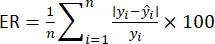         (21)

Results

            Distributed financial decision optimization (RQ1)

Centralized DRL reached the highest cumulative revenue but at the cost of poor privacy protection with a low privacy score of 0.30. In contrast, the proposed JLR framework achieved a cumulative revenue of 60.8 billion yuan, only 7% lower than centralized DRL, while maintaining a high privacy score of 0.92. In addition, it outperformed Independent RL and FedSL on decision stability. Thus, the proposed JLR framework p...

Discussion

The results demonstrate that the proposed framework effectively addresses three core challenges in distributed financial risk management: (i) privacy-preserving financial decision optimization, (ii) dynamic modeling of inter-enterprise risk contagion, and (iii) stakeholder-oriented interpretability under regulated data environments. Rather than treating these as isolated objectives, the framework couples joint reinforcement learning (JRL) with an adaptive graph neural network (AGNN) and a dual-channel explanation layer, ...

Materials

List of materials used in this article

Name	Company	Catalog Number	Comments
Financial Data Management Software	Wind Information Co., Ltd.	N/A	Provided quarterly financial data of 300 A-share companies (2018–2023)
GPU server	NVIDIA	Version A100	Hardware
High-Performance Computing Server	Dell Technologies	R7525	Used for running federated reinforcement learning and AGNN training experiments
Python		Version 3.1	Software
PyTorch	Meta AI	Version 2.1	Software
Ray RLlib		Version 2.6	Toolkit
SHAP		Latest Version	Library

References

- Goldfarb, A., Tucker, C. Digital economics. J Econ Lit. 57 (1), 3-43 (2019).
- Guo, Y. Contextualized design of IoT finance for operational risk in commercial banks. Comput Intell Neurosci. 2022, 1-11 (2022).
- Wieandt, A., Heppding, L. Centralized and Decentralized Finance: Coexistence or Convergence. The Fintech Disruption: How Financial Innovation Is Transforming the Banking Industry. , Palgrave Macmillan. Cham, Switzerland. (2023).
- Geng, X., Han, B., Yang, D., Zhao, J. Credit risk contagion of supply chain finance: An empirical analysis of supply chain listed companies. PLoS One. 19 (8), e0306724(2024).
- Li, B., Zhang, X. Systemic risk and financial networks. Q Rev Econ Finance. 94, 25-36 (2024).
- Cui, Y., et al. FraudGNN-RL: A graph neural network with reinforcement learning for adaptive financial fraud detection. IEEE Open J Comput Soc. 6, 426-437 (2025).
- Communication-efficient learning of deep networks from decentralized data. McMahan, B., Moore, E., Ramage, D., Hampson, S., Arcas, B. A. Y. Proc Int Conf Artif Intell Stat, 54, 1273-1282 (2017).
- Lundberg, S. M., Lee, S. -I. A unified approach to interpreting model predictions. Proc Neural Inf Process Syst. 31, 4768-4777 (2017).
- Adadi, A., Berrada, M. Peeking inside the black box: A survey on explainable artificial intelligence (XAI). IEEE Access. 6, 52138-52160 (2018).
- Lillicrap, T. P., et al. Continuous control with deep reinforcement learning. arXiv. , (2015).
- Hasan, M. M. Federated learning models for privacy-preserving AI in enterprise decision systems. Int J Bus Econ Insights. 5 (3), 238-269 (2025).
- Pisoni, G., Molnár, B., Tarcsi, Á Data science for finance: Best-suited methods and enterprise architectures. Appl Syst Innov. 4 (3), 69(2021).
- Kumar, R., Singh, M. K. Cross-jurisdictional privacy compliance in multi-cloud architectures: A framework for GDPR, CCPA, and PIPL alignment. Sci Pract Cyber Secur J. , In Press (2025).
- Kishor, K. Communication-Efficient Federated Learning. Federated Learning for IoT Applications. EAI/Springer Innovations in Communication and Computing. , Springer. Cham, Switzerland. (2022).
- Kumar, P. N., Umeorah, N., Alochukwu, A. Dynamic graph neural networks for enhanced volatility prediction in financial markets. arXiv. , (2024).
- Zhang, K., Yang, Z., Başar, T. Multi-Agent Reinforcement Learning: A Selective Overview of Theories and Algorithms. Handbook of Reinforcement Learning and Control. , Springer. Cham, Switzerland. (2021).
- Wu, Z., et al. A comprehensive survey on graph neural networks. IEEE Trans Neural Netw Learn Syst. 32 (1), 4-24 (2021).
- Barredo Arrieta, A., et al. Explainable artificial intelligence (XAI): Concepts, taxonomies, opportunities and challenges toward responsible AI. Inf Fusion. 58, 82-115 (2020).
- Dexiang, Y., Shengdong, M., Liu, Y., Jijian, G., Chaolung, L. An improved deep-learning-based financial market forecasting model in the digital economy. Mathematics. 11 (6), 1466(2023).
- Guendouzi, B. S., Ouchani, S., El Assaad, H., El Zaher, M. A systematic review of federated learning: Challenges, aggregation methods, and development tools. J Netw Comput Appl. 220, 103714(2023).
- Liu, T., et al. Efficient and secure federated learning for financial applications. Appl Sci. 13 (10), 5877(2023).
- Graph neural networks for advanced financial risk modeling in volatile markets. Narsepalle, K. R., Bolla, S. R. Proc Int Conf Eng Technol Manage, , 1-5 (2025).
- Integrated explainable AI for financial risk management: A systematic approach. Murthy, P., et al. Proc IEEE Int Conf Interdiscip Approaches Technol Manage Soc Innov, , 1-6 (2025).
- Duan, J., Zhou, J., Li, Y. Privacy-preserving distributed deep learning based on secret sharing. Inf Sci. 527, 108-127 (2020).
- Afzal, M. U., Abdellatif, A. A., Zubair, M., Mehmood, M. Q., Massoud, Y. Privacy and security in distributed learning: A review of challenges, solutions, and open research issues. IEEE Access. 11, 114562-114581 (2023).
- Lu, Y., Zhu, M. Privacy-preserving distributed optimization using homomorphic encryption. Automatica. 96, 314-325 (2018).
- Skarding, J., Gabrys, B., Musial, K. Foundations and modeling of dynamic networks using dynamic graph neural networks: A survey. IEEE Access. 9, 79143-79168 (2021).
- Beauty, A. M. Explainable AI in data-driven finance: Balancing algorithmic transparency with operational optimization demands. Int J Res Publ Rev. 2 (6), 125-149 (2025).
- Adaptive blockchain-driven IoT authentication for secure machine learning. Lin, J. Proc Int Conf Internet Things Mach Learn, , 324-330 (2025).
Access restricted. Please log in or start a trial to view this content.