Automated Ultradilute Measurements of Self-Association for the Identification of Antibodies with Favorable High-Concentration Solution Properties

Summary

Here, we describe a high-throughput adaptation of an antibody colloidal stability assay at scale to generate large datasets and support AI/ML-ready developability predictions.

Abstract

One of the key challenges in antibody engineering is the development of analytical screening methods to assess colloidal stability, ensuring that biologics are suitable for high-concentration formulation and administration. Charge-stabilized self-interaction nanoparticle spectroscopy (CS-SINS), a modified version of the conventional affinity-capture self-interaction nanoparticle spectroscopy (AC-SINS), has been adapted as a robust colloidal stability assessment for predicting high-concentration solution behavior. This method enables critical early-stage developability decisions by identifying colloidal stability issues before significant resources are invested, substantially reducing downstream attrition rates and accelerating candidate selection timelines. This study demonstrates that the assay seamlessly integrates into existing discovery workflows and can be performed in parallel with typical early-stage assays due to its minimal sample requirements, providing valuable data to predict high-concentration behavior without compromising other characterization efforts. It has been shown that routine dynamic light scattering (DLS) measurements, in addition to the shift in the plasmon resonance wavelength, can improve the reliability of the HTP method described here. Taken together, it is anticipated that the cross-validation using DLS measurements and automated analysis programs will facilitate the reliable selection of candidate antibody therapeutics of various modalities.

Introduction

In the development and formulation of therapeutic antibodies, opalescence and viscosity are key considerations in developing a patient-centric commercial product^{1,2,3,4,5,6,7,8}. Classically, large amounts of protein are required to directly observe these properties at high concentration, effectively preventing optimal lead identification during the early stages of antibody discovery, where protein availability is limited. Reliable identification of these phenomena is critical to developability assessments to mitigate poor high-concentration solution behavior downstream^{1,2,3,4,5,6,7,8}. As such, there is significant interest in high-throughput, low-concentration methods that are predictive of poor solution behavior at high concentration^{9,10,11,12,13,14,15,16}. One such method, kD-DLS, has been shown to be reliable for predicting high-concentration properties but does not meet the low protein consumption and high-throughput requirements of early-stage workflows^12,13.

Recently, an ultralow consumption gold nanoparticle-based assay known as CS-SINS has been shown to have a strong correlation with the results of the kD-DLS experiments and is reasonably effective at predicting poor solution properties at high concentration¹⁶. These characteristics make CS-SINS an ideal candidate for development as a high-throughput screening tool. The CS-SINS assay employs a capture antibody immobilized on gold nanoparticle surfaces to anchor candidate antibodies via their Fc regions, leaving the Fab arms accessible to solution interactions. This configuration means that Fab-Fab interactions dominate the measured self-association signal, which is advantageous since studies indicate that Fab domains contribute predominantly to mAb self-association characteristics, likely due to the complementarity-determining region (CDR) surface properties^{17,18,19,20,21,22,23}. This mechanistic basis makes CS-SINS well-suited for predicting colloidal stability risks relevant to high-concentration formulations. Alternative HTP methods, including standup monolayer adsorption chromatography (SMAC), a size exclusion chromatography (SEC) column-based approach that mimics self-association with a generic stationary phase, and cross-interaction chromatography (CIC), involve column preparation and large sample requirements^{17,24,25,26,27}.

The method described here details a plate-validated setup of the CS-SINS assay and enables HTP screening through lab automation and analysis, combining the advantages of existing methods while enhancing the reliability of the results. This study also demonstrates how various sample types yield high-quality results due to the nature of the enrichment of self-interaction in the assay, establishing that the method is agnostic to protein sources. Furthermore, we consider how earlier communication of colloidal properties to project teams can further support strategic multispecific antibody drug design^{28,29,30,31,32,33,34}.

The study of high-concentration solution properties is typically performed downstream in multispecific candidate selection campaigns, after lead selection and completion of engineering (Figure 1A). Early prediction of these properties has become feasible with methods such as CS-SINS that require a few micrograms of sample, thereby predicting colloidal stability risks with ultradilute measurements¹⁶. The introduction of early developability screening (Figure 1A), when the candidate pool is large, and parallel data generation campaigns for both monospecific and multispecific formats could better inform the drug discovery process^31,32. HTP CS-SINS fits into the existing molecule screening paradigm in parallel to binding and function determination, therefore adding to the information package without disrupting or holding up existing workflows. Lead candidate selection with emphasis on favorable colloidal properties will impact the selection progression as represented in Figure 1B.

In the proposed early developability screening workflow, lead identification considers the full picture for favorable drug properties, including manufacturing and patient access, thus streamlining downstream development³⁴. The high-concentration properties of biologics can determine their route of administration: intravenous injections that require hospital visits or subcutaneous injections, which can be administered at home by the patient, but often require a high-concentration product^35,36. Developable mAbs with low self-association are often formulated at >100 mg/mL^5,35. Formulation optimization using excipients, such as visco-reducing agents, can overcome colloidal stability risks for desirable candidates with poor solution properties at the CMC development stages^34,35. However, this introduces downstream challenges in biopharmaceutical manufacturing and increases timelines to successful drug approvals³⁶. Excipients known to lower viscosity (such as salts and amino acids) can also affect protein stability, altering the previously characterized developability profiles and complicating the process further^36,37. Additionally, excessive excipients can limit the patient population due to immunogenicity considerations, various safety concerns, or affect treatment adherence and can introduce new challenges in the production space^38,39,40. Starr et al. published the CS-SINS method for the first time, describing the optimal mass fraction of PLL and IgG to be 0.03 and confirming nanoparticle stabilization by zeta potential measurements for mAb self-association in histidine formulations¹⁶. Notably, adding too much PLL creates overstabilization in the assay and prevents the observation of mAb self-interaction (gold nanoparticle stability improvement by PLL is depicted in Supplementary Figure 1). The use of histidine formulations without salt minimizes electrostatic screening (increasing the Debye length), which extends the range of intermolecular interactions, thereby amplifying weak self-association signals and mimicking high-concentration behavior where antibodies are in closer proximity. In general, low ionic strength formulations are preferred for high-concentration formulations where self-association is not observed.

Large PLL polymers prevent the occupation of more capture mAbs at the gold nanoparticle surfaces, which narrows the plasmonic shift window and requires a more sophisticated curve-fitting program and analysis for subsequent data analysis. This study utilized a web portal tool that syncs with internal databases. The major advantage of this up-front cost is the data-building potential from a large sequence pool to maximize the diversity of candidates downstream and mitigate bottlenecks at the costlier development stages^34,35,36. The CS-SINS assay we describe here stands out as an HTP-compatible method, which has been shown to correlate well with late-stage colloidal stability assays¹⁶. AI-assisted profiling is in progress for the thoughtful design of multispecifics for future programs and for the understanding of the individual contributions of each domain in complex formats^41,42,43,44. These efforts will collectively influence meta-analyses and a more detailed determination of colloidal stability properties for antibody therapeutics, and therefore ultimately save time at the early R&D stages.

Protocol

Figure 2 depicts the nanoparticle conjugation preparation, Figure 3 depicts the workflow in its entirety, Figure 4 maps out the lab automation process, and Figure 5 contains a diagram of the data analysis pipeline. The reagents and the equipment used are listed in the Table of Materials.

1. Preparation of buffers

NOTE: Week 1 (sample preparation)

1. Prepare histidine (10 mM), pH 6.0 (sample and assay buffer).
   NOTE: These steps are performed on Day 1.
   1. Dissolve 5 mM L-histidine monohydrochloride monohydrate and 5 mM L-histidine in ultrapure water. Add hydrochloric acid dropwise while stirring until the pH reaches 6.0, as measured with a calibrated pH meter.
   2. Filter the solution through a 0.22 µm pore-size filter under vacuum and collect the filtrate in a sterile bottle.
   3. Measure the conductivity for quality control purposes and ensure a reading of approximately 500 µS/cm.
2. Prepare potassium acetate (20 mM), pH 4.3 (capture mAb conjugation buffer).
   1. Dissolve potassium acetate in ultrapure water and adjust the pH to 4.3 with glacial acetic acid.
   2. Sterilize the solution by vacuum filtration through a 0.22 µm pore-size filter as described in step 1.1.2.
3. Prepare poly-L-lysine.
   1. Prepare a 5 mg/mL stock solution in ultrapure water and store at −20 °C until use.

2. Dialysis of all samples (candidate mAbs)

NOTE: Perform these steps on Days 2–5.

1. Pre-soak 100 µL or 300 µL dialyzers in 10 mM histidine, pH 6.0, for 5 min.
2. Transfer all samples (50–100 µL) to dialysis cassettes. Submerge the cassettes in 10 mM histidine buffer, pH 6.0 (700 mL per box), add stir bars to the reservoirs, place the reservoirs on magnetic stirring plates, and incubate at 4 °C for 2 h 15 min.
3. Perform seven buffer exchanges with 10 mM histidine, pH 6.0, every 2 h 15 min, or perform four overnight buffer exchanges to ensure thorough removal of salt from the samples.
4. Retrieve the samples, transfer them to clean matrix vials, and store at 4 °C until the CS-SINS assay is performed.
5. Measure the sample concentrations and record the polydispersity information after dialysis. Calculate the corrected concentrations by dividing the raw absorbance values at 280 nm by the absorbance at 280 nm for a 1 mg/mL solution.
6. Prepare the liquid-handler input file with the well addresses and concentrations (µg/mL), including the controls.

3. Buffer exchange of capture mAb (Figure 2, step 1)

NOTE: Perform these steps on Day 1 of Week 2 (assay).

1. Remove the storage buffer from 2 mL desalting columns by centrifuging for 2 min at 1,000 × g at room temperature. Prepare two desalting columns for every 700 µL of capture mAb required. Discard the flow-through after each centrifugation step.
2. Wash the columns three times with 1 mL of 20 mM potassium acetate buffer, pH 4.3. Centrifuge the columns for 2 min at 1,000 × g during each wash.
3. Add 700 µL of capture mAb (goat anti-human Fcγ-specific antibody) to each column and elute into a fresh 15 mL tube by centrifuging for 2 min at 1,000 × g.
4. Collect the desalted eluate, apply it to a second equilibrated desalting column, and centrifuge for an additional 2 min at 1,000 × g.
5. Combine all eluted samples.
6. Measure the concentration of the capture mAb solution after desalting as described in Days 2–5, step 2.5.
7. Dilute the capture mAb stock solution to 0.8 mg/mL with 20 mM potassium acetate buffer, pH 4.3, and set aside until use.

4. Preparation of a working stock of poly-L-lysine

1. Dilute a small aliquot of the poly-L-lysine stock solution to 2.66 mg/mL with ultrapure water.

5. Concentration of gold nanoparticles (Figure 2, step 2)

1. Prepare 1.2 mL aliquots of the stock suspension in 1 mL tubes or 4.8 mL aliquots in 5 mL tubes using polypropylene microcentrifuge tubes containing 20 nm gold nanoparticles. Centrifuge at 21,130 × g for 6 min.
2. Remove the supernatants (~1.1–1.15 mL) without disturbing the pellets and transfer them to a separate conical tube.
3. Combine the concentrated pellets and residual volumes in a clean microcentrifuge tube. Determine the nanoparticle volume by pipetting and adjust the volume to (number of 1 mL tubes × 50 µL) or (number of 5 mL tubes × 200 µL) using the reserved supernatant. For example, after centrifuging 10 aliquots of 1.2 mL in 1 mL tubes, adjust the final volume of the concentrated nanoparticles to 500 µL.

6. Nanoparticle assembly

1. Thoroughly mix 1.5 µL of the poly-L-lysine working solution with 48.5 µL of the buffer-exchanged capture mAb (Figure 2, step 3).
2. Prepare a 1:1 mixture of the concentrated nanoparticle solution from step 5 and the poly-L-lysine/capture mAb solution from step 6.1 (Figure 2, step 4).
3. Incubate the mixture overnight at room temperature (23 °C) (Figure 2, step 5).

7. Liquid-handler assay plate set up

NOTE: Perform these steps on Day 2.

1. Compile the materials required for the assay, including dialyzed antibodies, the liquid-handler input file containing post-dialysis concentrations, conjugated gold nanoparticles, robotic handling tips, plates, and reservoirs (Figure 3, Lab Automation, step 1). Preload the tips, samples, plates, and reservoirs onto the deck according to the layout shown in Figure 3 (Lab Automation, step 1).
2. Add the controls to wells A12–D12 of the sample plate (two positive controls and two negative controls). Leave well H12 empty for the buffer sample prepared by the liquid handler.
3. Open the liquid-handler CS-SINS method and start the program (Figure 3, Lab Automation, steps 2–3). Load the liquid-handler input file when prompted and enter the number of samples (Figure 4A). Review the two subsequent calculation-check windows (Figure 4B,C), confirm the values, and proceed with the run.
4. Normalize the samples, including the controls, to 55.5 µg/mL in 10 mM histidine buffer, pH 6.0, by transferring them from the matrix sample tubes to the polymerase chain reaction plate in a final volume of 100 µL (Figure 4D, step 1). Monitor the progress, noting that completed plate areas appear grey and active steps are highlighted in green (Figure 4E).
5. Prepare a larger-volume dilution of each sample at 11.1 µg/mL in 10 mM histidine buffer, pH 6.0, by transferring material from the polymerase chain reaction plate to a deep-well block at a final volume of 200 µL (Figure 4D, step 2).
6. Allow the system to pause after step 2. When prompted, mix the concentrated gold nanoparticles prepared in step 6.3 by inverting the tube and pipetting up and down approximately 10 times.
   1. Distribute the nanoparticles evenly between two polypropylene microcentrifuge tubes and place the tubes, with caps open, in the designated tube-rack location on the deck (Figure 4D, highlighted “AuNP”). Resume the run and allow the liquid handler to dispense 20 µL of nanoparticles into each well of the second deep-well block, two wells at a time (Figure 4D, step 3).
7. Allow the liquid handler to transfer 192 µL of sample from the deep-well block containing the 11.1 µg/mL samples (Figure 4D, step 2) to the second deep-well block and mix thoroughly. Generate a 4× CS-SINS mastermix for each sample, resulting in a final sample concentration of 10 µg/mL after the addition of 48 µL of gold nanoparticles to a final volume of 240 µL (Figure 4D, step 3). Start the 4 h incubation timer at this point.
8. Allow the liquid handler to dispense 30 µL into the source well and then dispense 60 µL into three of the four wells in each quadrant of a 384-well plate to generate technical triplicates for each sample (Figure 4D, step 4). Return the remaining 30 µL to the source plate.
9. Monitor the liquid-handler deck layout as the run progresses. Observe the used tips and filled sample wells changing from light to dark grey in real time, while active movements are indicated in green (Figure 4E).
10. Remove the plate after completion of the run. Seal the plate with a minimally adhesive transparent plate seal and incubate at room temperature for a total of 4 h. At the 3.5 h time point, start the dynamic light scattering program to equilibrate the chamber to 20 °C using the settings shown in Supplementary Figure 2.
11. Measure the absorbance spectrum of each well from 510 to 570 nm in 1 nm increments (30 nm on each side of the peak) at the 4 h time point.
12. Immediately measure the plate using the dynamic light scattering plate reader at the 4.5 h time point with the settings shown in Supplementary Figure 2.
    NOTE: Use a high-performance plate reader for spectral measurements because of the limited dynamic range. Do not use the speed-read function.

8. Data analysis (Figure 5, Data processing scheme)

1. Export the raw files from the spectrophotometer platform and save them to an accessible drive folder.
2. Access the scripting web portal linked to the internal server. Enter the required CS-SINS input parameters, including: (1) Starting wavelength; (2) Directory location of the raw results file; (3) Plate-set and candidate identifiers; (4) Positive- and negative-control well addresses for normalization; (5) Method setup designation ("Manual" or "Liquid handler"); (6) Instruments used for spectral scanning and dynamic light scattering measurements; (7) Electronic laboratory notebook (ELN) identifier; (8) Acquisition date.
3. Submit the parameters to the web portal and verify that three Excel files are generated in a subfolder of the raw-results directory.
4. Calculate the λmax values using the curve-fitting script executed by the web portal.
5. Review the two output files containing replicate values, normalized results, and representative graphs for the spectral scan and dynamic light scattering measurements.
6. Use the third output file, containing assay metadata and normalized results, to create bulk laboratory results in the database user interface. Define reporting attributes according to group-specific requirements and upload the results to the database to enable company-wide access.

Results

Figure 6 shows the results, Supplementary Figure 3A shows an example of CS-SINS score from a representative crude and purified sample, Supplementary Figure 3B depicts the variability in signal from well-to-well across different days, Supplementary Figure 4 contains the results from the plate validation process, and Supplementary Figure 5 describes the normalization calculation for both CS-SINS readouts.

Importantly, samples were collected with reported concentrations of at least 55 µg/mL post dialysis into 10 mM Histidine, pH 6.0, for assay feasibility, since this is the minimum stock concentration (a minimum of 6 µg per sample) and created new child identifiers. In total, there were 70 purified samples and 20 crude expression samples, each representing sample types at different developability checkpoints (purified at the lead optimization stage and 1- or 2-step purified crude material from lead identification stage highlighted in Figure 1A). Crude material was generated from a fully automated mammalian expression system, Protein Expression and Purification Platform (PEPP; GNF, San Diego, CA, USA). The controls were derived from commercial material and were previously validated as having maximal or minimal viscosity, kD-DLS, and CS-SINS values. Fresh aliquots are stored at -80°C, and a new aliquot is used for each assay.

Figure 6A,B show the average spectral and DLS scores plotted by sample type, and the bar graphs display error bars (standard deviation) with matching color codes. The normalization is calculated by the script by dividing the difference between the sample and the negative control values (calculated lambda max by spectral shift or Z-average, hydrodynamic diameter in nm) by the difference between the controls (Supplementary Figure 5). Figure 6C plots the spectral scores against the DLS scores, depicting a clear correlation between the analytical approaches. Table 1 lists the identifiers, well addresses, sample type, spectral scores, and DLS scores along with their standard deviations for reference. The cutoff for colloidal stability risk (regardless of spectral or DLS reading) for a monospecific IgG is anything higher than a normalized value of 0.35 (indicated by a green dotted line in Figure 6A,B, 6/70 (excluding replicate controls) purified samples scored high-risk, while 64/70 scored low for the purified material. Importantly, we would expect the cutoff to trend higher for multispecific formats. For the crude expression samples, 2/20 samples scored high, while 18/20 scored low. Of the purified materials tested here, crude expression of parental batches of a subset was also screened and yielded similar results (depicted in Supplementary Figure 3A), indicating the assay's representative nature upon scale-up (purification) of candidate proteins from independent batches. Despite limiting sample sizes, it is noted that the standard error can trend higher for the crude PEPP samples than the purified samples. The benefit of performing CS-SINS at the later stages ensures that orthogonal assessments can be performed with assays requiring more protein for analysis, such as viscosity and kD-DLS measurements, while the benefit of performing CS-SINS in early developability screens pre-emptively addresses colloidal stability risks, potentially influencing the final lead candidate pool (Figure 1B). Borderline candidates with high error can be confirmed as high or low risk with assays downstream.

Due to the small nature of the plasmonic shifts being detected, an alternative readout was described to instill confidence in the assay, which broadens the dynamic range, which could prove particularly useful in the absence of a high-end plate reader to detect minute changes. The DLS readout distinguishes between nanoparticle clustering and reliance on the nanoparticles' spectral properties; however, both descriptors have similar standard error ranges and are small relative to their measurements. It appears that samples more prone to outlier readings will have higher error (or be “multimodal” and not report a result by DLS), but CS-SINS values within the working range of the assay have low error distributions. When comparing DLS values to spectral score values, the error distribution is tighter for the DLS results taken from crude samples than for the spectral scores; however, this only made a difference for 1 candidate that fell below the cutoff as a DLS score but not as a spectral score. This could prove useful if labs have different instruments available.

To specifically address the reliability of the data processing and the method itself, the scan times were modified from end-to-end for both readouts for the positive and negative controls in the dataset above, in addition to multiple medium and low controls to serve as intermediate reference points at the beginning and end of a 384-well plate. Supplementary Figure 4 depicts the results from the finalized plate validation, showing mostly insignificantly different values from the samples placed at the beginning versus the end of the plate (Supplementary Figure 4A,B) and high correlation between both readout values (Supplementary Figure 4C). Finally, the Z-factor and %CV were calculated for the controls from the spectral scanning and the DLS dataset in Figure 6. From the data generated for the controls and presented here, the spectral scan readout was determined to have a Z-factor of 0.648, with 0.019% CV for the positive control and 0.012% for the negative control. For the DLS readout, a Z-factor of 0.998 was calculated, with 0.025% CV for the positive control and 0.021% for the negative control. Overall, the Spearman correlation coefficient between sample values in this assay (Figure 6C) was calculated to be strongly positive at 0.829. These values represent solid precision and reproducibility for both measurement types, and unsurprisingly, the new, advantageous DLS detection strategy optimizes the Z-factor, but the spectral scan provides a sufficient separation band for recording reliable results (Z > 0.5). It is important to note that the DLS score is an orthogonal readout collected simultaneously within the CS-SINS workflow, requiring no additional sample preparation. The larger difference in values for raw DLS scores accounts for an improved Z-factor, but the “scores” are interpreted the same because they are normalized from raw values. Furthermore, DLS readings capture three-dimensional sizes of nanoparticle clusters versus indirect indications of proximity from plasmonic shift and spectral information, which may strengthen our understanding of the CS-SINS assay dynamics. Considering the plate-based and time-critical nature of an HTP assay, we aimed to increase the reliability of the assay with these methods.

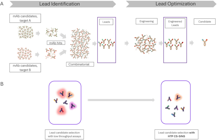
Figure 1: Developability paradigm and CS-SINS data collection. (A) The typical workflow from a discovery campaign to candidate selection is depicted for multispecific antibodies in this diagram. The discovery process results in monospecific candidates to screen, followed by vetting from various data packages to narrow down monospecifics of interest before combining into multispecific formats. Data packages are repeated or expanded upon to narrow down lead candidates until the best candidate is chosen for development. Lower throughput assays are performed in the current workstream when a small panel of molecules is selected (purple boxes). HTP CS-SINS can be performed at every stage along the path, adding valuable data and improving the selection process. (B) The hypothetical outcome of colloidal properties for the top 6 candidates is shown for 2 possible paths: lead candidate selection with low-throughput assays, and lead candidate selection with HTP CS-SINS. Candidates with unfavorable solution behavior are represented with a glow. In the first scenario, half of the lead candidates based on optimal binding characteristics from discovery screens display poor high-concentration behavior. In the second scenario, only 1 candidate with moderately poor colloidal stability is included, because CS-SINS data was considered in parallel to binding data in early discovery screens. In the second scenario, the diversity of potential viable candidates is higher than in the first scenario. Please click here to view a larger version of this figure.

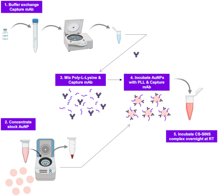
Figure 2: SINS assay workflow. Gold nanoparticle preparation and conjugation: (1) The capture mAb is buffer-exchanged into 20 mM potassium acetate, pH 4.3, and diluted to 0.8 mg/mL. (2) Gold nanoparticles are concentrated from the stock. (3) Poly-l-lysine is mixed with the buffer-exchanged capture mAb. (4) Gold nanoparticles are incubated with the poly-l-lysine and capture mAb, and thoroughly mixed. (5) Incubation of CS-SINS complex overnight at room temperature. Please click here to view a larger version of this figure.

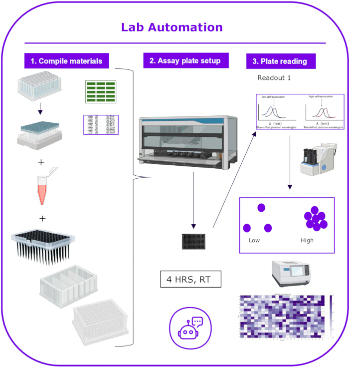
Figure 3: Lab Automation workflow. Lab Automation workflow: (1) Materials and samples are compiled for the liquid handler method. Dialyzed samples in 10 mM Histidine, pH 6, are collected in matrix tubes or 96-well plates. Sample concentrations are formatted into a liquid handler input file. CS-SINS complex gold nanoparticles conjugated to capture mAb, robotic liquid handling tips, and plasticware are gathered in preparation for the liquid handler assay setup. (2) The assay plate is prepared on the liquid handler and incubated for 4 h at room temperature. 3) At the 4-h mark, spectral scans (readout 1) are collected from sample wells spanning 25 min; after the 4.5-h mark, dynamic light scattering (readout 2) collects size information on each more uniform well population. Please click here to view a larger version of this figure.

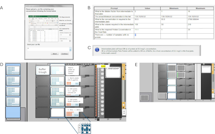
Figure 4: Liquid handler program and plate setup. (A) Upon program start and after the system initializes, a separate window/prompt will open up to select the input file with the designated well addresses and sample concentrations. The number of samples must be specified each time, but the 200 µL volume (the final volume of the mixed reagents prior to 384-well plate stamping) stays the same. (B) After clicking continue from the prior window in (A), this second window will appear to confirm the interpretations from the input file on the left and values on the right. (C) After confirming the interpretations from (B), this third window appears with a dialogue box double-checking the math for sample concentration for normalization (the 100 µL volume ) to the final deep well plate (the 200 µL volume ). (D) This layout comes from the Method Editor view of the liquid handler software module. On the left, 300 µL standard tips are loaded, and in the center of the stage, 1 box of 50 µL, and 3 boxes of 300 µL slim tips are loaded, which are compatible with liquid handling robotics. A buffer trough is loaded in the front with 10 mM Histidine, pH 6 (the buffer that the samples were dialyzed into). The Gold nanoparticles are split evenly into 2 microcentrifuge tubes and loaded, uncapped, in the back of the tube rack on the right. The matrix plate with sample tubes is loaded in the back of the carrier in column 10. Following the samples, the normalization plate (1), deep well plate with 11.1 µg/mL sample (2), 200 µL deep well plate of the combined sample and nanoparticles (3), and 384-well formatted plate (4) are indicated. (E) The liquid handler deck layout shows the retrieval of tips and sample dispensing in real-time and marks the wells as each step progresses. Here, all samples (96-well image at the back of the carrier in the 3^rd column), are greyed out as well as the subsequent normalization plate, which indicates that samples have been added to the normalization plate from the source matrix plates. In green, we show the 8-channel head after aspirating buffer from the trough and dispensing it into the first column of the normalization plate while mixing. Please click here to view a larger version of this figure.

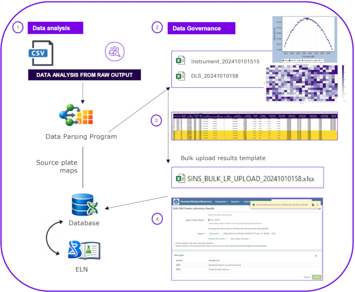
Figure 5: Data processing scheme. The data processing scheme: (1) The raw data files are submitted to an internal server. (2) The data files are read and processed by a script customized to finetune curve-fitting of spectral scans, calculate the lambda max for CS-SINS replicates, and vet multimodal populations by DLS. (3) The data is grouped by replicates, then subsequently averaged and normalized to specified controls; matching plate maps in the database portal are sourced to link the results. (4) All data is organized into a template ready to upload to the database, and graphs are automatically created for ELN reporting. Please click here to view a larger version of this figure.

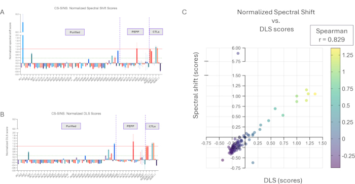
Figure 6: Representative data from readout 1 and readout 2. (A) The normalized spectral shift scores were plotted by PPB ID for purified, crude expression samples, and control samples where indicated and separated by a vertical dotted line, in a bar graph plot to determine error bar distribution among sample types. The solid red line indicates the upper limit of the assay, which corresponds to the positive control, while the green dotted line marks the cutoff value for a low-risk molecule profile for CS-SINS. (B) The normalized DLS scores were plotted by PPB ID for purified, crude expression samples, and control samples, where indicated and separated by a dotted line, in a bar graph plot to determine error bar distribution among sample types. Some values are missing (such as the 2^nd value in light blue with an above-average score in (A) due to multimodal scans from the DLS output, which the scripting software web portal determined to be invalid. The solid red line indicates the upper limit of the assay, which corresponds to the positive control, while the green dotted line marks the cutoff value for a low-risk molecule profile for CS-SINS. (C) The averaged, normalized scores for spectral shift and DLS values were compared by a correlation dot plot, as shown (spectral shift scores correspond to the Y-axis and DLS scores correspond to the X-axis). The color code is coordinated with DLS scores only. Please click here to view a larger version of this figure.

Table 1. Colloidal stability scores of antibody samples determined by CS-SINS. The table summarizes sample identifiers, well addresses, sample classifications, normalized spectral scores, and dynamic light scattering (DLS) scores obtained from the CS-SINS assay. Please click here to download this Table.

Supplementary Figure 1: PLL improved the stability of AuNP in 10 mM His buffer, pH 6, for CS-SINS. This figure depicts the close overlay of the negative control mAb bound to the PLL-coated CS-SINS complex and buffer-only control in contrast to uncoated gold nanoparticles with the negative control mAb or buffer alone, which have peaks in entirely different ranges. Shown in blue are the incremental spectral scans (taken in 1 nm increments at the 4-h timepoint) for conjugated AuNP incubated with 10 mM His buffer overlaid with conjugated beads incubated with the negative control (PPB-117487) in the absence of a pre-incubation of poly-l-lysine. Show in red are the incremental spectral scans (taken in 1 nm increments at the 4-h timepoint) for conjugated AuNP incubated with 10 mM His buffer overlaid with conjugated beads incubated with the negative control (PPB-117487) after pre-incubation of poly-l-lysine. Calculated lambda max for both negative controls in the presence of PLL are close together. Please click here to download this file.

Supplementary Figure 2: Settings for DLS and well plate selection for the DLS plate reader. Please click here to download this file.

Supplementary Figure 3: CS-SINS scores from Abs expressed in PEPP vs. Purified downstream. (A) The normalized spectral shift scores were plotted by well and plate ID for PEPP samples (eg, A1PL1 = well A1 from plate 1) expressing Ab64 and separated by a vertical dotted line from the normalized spectral shift or DLS scores from purified Ab64 downstream, in a bar graph plot to determine error bar distribution (standard deviation) among sample types. The green dotted line marks the cutoff value for a low-risk molecule profile for CS-SINS. (B) The total AUC and distribution across the plate for all samples in the experiments run in (A) are plotted here (color-coded for corresponding experiments). Please click here to download this file.

Supplementary Figure 4: End-to-end 384-well plate validation of controls. (A) The averaged, normalized spectral scores for samples in the beginning columns of the 384-well plate are plotted and shown in red, while duplicate values scanned at the end of the 384-well plate are shown in lime green. Replicate values are side-by-side, ranging from the positive control (indicated with a plus sign next to the PPB ID) to the negative control (indicated with a minus sign next to the PPB ID). The value for the buffer control prepared by the liquid handler program (independent from the sample input prompt) is shown in a checkered pattern. (B) The averaged, normalized DLS scores for samples in the beginning columns of the 384-well plate are plotted and shown in red, while duplicate values scanned at the end of the 384-well plate are shown in lime green. Replicate values are side-by-side, ranging from the positive control (indicated with a plus sign next to the PPB ID) to the negative control (indicated with a minus sign next to the PPB ID). There is no buffer control value for the DLS readout (due to multimodal readings). (C) The averaged, normalized spectral scores are plotted against DLS scores in a correlation dot plot for samples ranging from readings in the beginning columns of the 384-well plate to the end of the 384-well plate. The color coding for the datapoints corresponds directly to the average, normalized spectral scan scores. Since there is no buffer control value for the DLS readout (due to multimodal readings), only the 6 controls in duplicate are compared from both readouts in this plot. Please click here to download this file.

Supplementary Figure 5: The calculations for the normalization of spectral scores or DLS scores to enable universal reporting and referencing between users and days. Positive control values are set to a value of 1, while negative controls are set to a value of 0, and high scores are associated with poor colloidal behavior. Please click here to download this file.

Discussion

This protocol represents several key modifications from the original CS-SINS method¹⁶. Importantly, the optimized PLL:IgG ratio and histidine buffer were maintained from the original study¹⁶. Most notably, the assay was adapted for the liquid handler robotic platform to enable HTP processing (up to 352 samples in 1 day versus ~20), reducing hands-on time and improving reproducibility through automated liquid handling. The robotics system is compatible with plate-based formats, including stamping into new formats such as the 384-well plate, and various labware types. The programs can run independently, and the end-to-end workflow provides a high-volume readout with enhanced reproducibility in a sample-limiting setting. DLS measurements were also incorporated as an orthogonal readout to the spectral shift with a more optimal Z-factor than spectral shift interpretations (0.998 versus 0.648), which proves particularly valuable for samples with borderline spectral scores or high standard deviations, and describes the interpretation of the plasmon shift to enhance the dynamic range apparent from the plate reader output alone. It is suggested that labs without high-end multimode plate readers available could use DLS to reliably perform CS-SINS. To address potential time-dependent variability across a 384-well plate, extensive plate validation was performed (Supplementary Figure 4) by placing controls at both the beginning and end of the plate, confirming minimal scan time effects. Additionally, it was demonstrated that crude PEPP samples yield comparable results to purified material (Figure 6, Supplementary Figure 3A), expanding the applicability of the method to earlier discovery stages where purified protein is unavailable, which had not been previously reported. The data in Supplementary Figure 3 points to sample reliability between sources but also indicates minimal assay variability from day to day since the data was collected and normalized from different datasets. More specifically, Supplementary Figure 3B depicts the total area under the curve for all wells from respective experiment plates (color-coded to match the plate from the same experiment in Supplementary Figure 3A) to demonstrate the expected, yet minimal variability within the same experiment and on different days with distinct bead preparations. At the early discovery stage, methods such as kD-DLS and column-based approaches (SMAC, CIC) are not feasible due to higher sample consumption requirements and an inability to process crude material^{12,13,24,25,26,27}; CS-SINS uniquely enables colloidal stability screening at this stage with only 6 µg per sample, which can be 1-step purified. Finally, the curve-fitting script was updated to accommodate finetuning of minor lambda max shifts and to enable improved file handling and automated data reporting to internal databases.

Common troubleshooting scenarios include: (1) high standard deviations in spectral or DLS scores, often indicating incomplete mixing of nanoparticles (step 7.6) or sample aggregation - in such cases, it is recommended performing a QC check against the dialyzed samples by DLS to ensure integrity post-dialysis and defaulting to spectral scores as the standard readout; (2) multimodal DLS distributions or failed DLS readings, typically caused by pre-existing sample aggregation or dust contamination - filtration through 0.22 µm filters prior to dialysis can mitigate this; (3) discrepancies between spectral and DLS scores, which is typically attributable to skewed DLS measurements (likely due to high polydispersity, which would show up within the normal-high range by spectral score); (4) inconsistent positive control values, usually resulting from improper nanoparticle storage or degraded capture mAb; fresh aliquots stored at -80 °C should be used for each assay (not stored at 4 °C for more than a few days).

Some limitations of the assay include the need for time to dialyze samples thoroughly and prepare conjugated nanoparticles semi-manually the day prior to the assay; however, dialysis time is equivalent regardless of sample set size. With regards to tip clogging risks, the liquid handling tips monitor pressure changes during aspiration, and relevant errors would appear during operation. During the method development phase, we checked log files (and continue to after service) to ensure that expected volumes are being calculated by the script. The aliquoting functions have been tested for the concentrated bead preparations and do not anticipate issues. We acknowledge the time-sensitive nature of the assay, the Fab-dominated nature of the assessment, and its role as a surrogate assay without directly measuring colloidal behaviors such as viscosity and opalescence. However, this adaptation enables efficient characterization of larger datasets earlier in the drug discovery process, serving as a powerful screening tool where none previously existed.

Several critical steps in this protocol require careful attention to ensure reproducible results. First, precise pH adjustment during buffer preparation (steps 1.1.1 and 1.2.1) is essential, as deviations beyond ±0.1 pH units can affect nanoparticle stability and antibody capture efficiency. The low pH buffer used for capture antibody preparation ensures optimal conjugation, and the buffer conditions specified were optimized for charge stabilization and broad antibody compatibility (typically in a formulation context). The 10 mM histidine pH 6.0 buffer provides optimal electrostatic interactions while maintaining protein stability. Second, thorough dialysis with complete salt removal (step 2.3) is crucial; incomplete dialysis can interfere with electrostatic interactions during nanoparticle assembly. Third, the gold nanoparticle concentration step (protocol steps 5.1–5.3) must be performed carefully to avoid disturbing the pellet, as inconsistent nanoparticle concentrations directly impact assay sensitivity. Fourth, the PLL:capture mAb ratio of 0.03 (step 4.1) is optimized for maximal surface coverage while maintaining a sufficient plasmonic shift window, as previously established¹⁶. With respect to liquid handling dynamics, liquid sensing tips were utilized to perform normalizations and plate mixing up until gold nanoparticles are introduced, which are not reliably measured in solution (and therefore set dispensing volumes to standard amounts). Liquid sensing upstream allows for issues with plate misalignment or missing samples to be flagged by the operator, while the 384-well stamping step will identify Z-alignment issues. Finally, strict adherence to the 4-h incubation timing (protocol steps 7.10–7.12) and consistently reading the plate from beginning to end (regardless of an incomplete plate) is critical, as the plasmonic shift and nanoparticle clustering are time-dependent phenomena; delays or early readings can lead to inaccurate CS-SINS scores, while reading the full plate ensures consistency of scores across days in the HTP format.

As the colloidal stability of multispecific antibodies is increasingly investigated, the large datasets provided by HTP biophysical assays like CS-SINS have the potential to feed AI/ML models to better understand combinatorial effects on molecule stability. Studies have shown that as sequence diversity increases, the need for larger datasets increases to improve the accuracy of AI/ML results^41,42,43. Properties and molecular descriptors for monospecifics might change when reformatted into bispecifics or trispecifics, considering the whole molecule charge distribution and balance as opposed to sequence or motif-specific considerations for attributes such as chemical degradation liabilities^{17,18,19,20,21,22}. Notably, structural features such as predicted electrostatic patches, hydrophobicity, and solvent-accessible surface area can improve predictions of aggregation and stability independent of sequence-specific characteristics, making several smaller datasets compatible with prediction preparation^{17,18,19,20,21,22}. The simplicity of the CS-SINS score as a reference to the representative culmination of a molecule's biophysical profile makes the assay suitable for training AI/ML models.

Materials

List of materials used in this article

Name	Company	Catalog Number	Comments
CLEARSEAL FILM 100PKCLEARSEAL	Fisher Scientific	500214
CO-RE II (50 μL Conductive Tips, 300 μL Conductive Tips, 300 µL Slim Conductive Tips)	Hamilton Company	235966, 235902, 235806
Eppendorf Tubes Snap Cap (5.0 mL, Microtube)	Eppendorf	30119401
Falcon Conical Centrifuge Tubes (15 mL)	Thermo Fisher Scientific	Falcon 352196
Goat antihuman Fcγ-specific antibody	Jackson ImmunoResearch Laboratories	109-005-008
Gold nanoparticles (20 nm)	Ted Pella Inc.	157051
Greiner Bio-One 384-well μClear Bottom Polystyrene Microplates – (SS & DLS assay plates)	Fisher Scientific	07-000-057
Greiner Bio-One MASTERBLOCK 96 Deep Well Conical Bottom 2 mL Storage Plate – (mastermix and reagent mixing plates)	Fisher Scientific	07-000-122
Hard-Shell PCR Plates normalization (96-Well, low profile, thin wall, skirted, white/clear HSP9601)	Bio-Rad	HSP9601	URL: https://www.bio-rad.com/en-us/sku/HSP9601-hard-shell-96-well-pcr-plates-low-profile-thin-wall-skirted-white-clear?ID=HSP9601
Histidine hydrochloride buffer sample (10 mM, pH = 6.0, sample and assay buffer)	Sigma	H8125; H6034	Prepare final concentration of 5 mM per reagent in ultra-pure water, adjust pH to 6.0, adjust final volume with ultra-pure water, and filter with 0.22 μm filter
Matrix ScrewTop Tubes sample (500 μL)	Thermo Fisher Scientific	3744
MD100 or MD300 Xpress Mini Dialyzer (Xpress Micro Dialyzer, Scienova, 6-8 kDa, 96 pcs. in deep well plate (12 cartridges), sealing sheet) and dialysis reservoir/box (low volume dialysis cassettes)	Vivaproducts, Inc.	40789, 40076
Microcentrifuge tubes pure polypropylene (1.5 mL)	USA Scientific	1615-5500
Nalgene Disposable Polypropylene Robotic Reservoirs – (buffer trough)	Thermo Fisher Scientific	1200-2300
Nalgene Rapid-Flow Sterile Disposable Filter Units with PES Membranes	Thermo Fisher Scientific	567-0020
Poly-L-lysine, >70,000 MW	MP Biomedicals	219454405	Prepare a 5 mg/mL stock solution in ultra-pure water
Positive and negative Controls (1 mg/mL dialyzed into 10 mM Histidine, pH 6)	Internally-produced commercial antibodies	N/A	~2 nm spectral shift and DLS size of 250-300 nm for positive control; negligible spectral shift and DLS size comparable to buffer only control
Potassium acetate buffer capture (20 mM, pH = 4.3, mAb conjugation buffer)	Fisher Scientific	P171-500	Prepare final concentration of 10 mM reagent in ultra-pure water, adjust pH to 4.3 with acetic acid, adjust final volume with ultra-pure water, and filter with 0.22 μm filter
Zeba desalting columns (2 mL, 5 mL, or 10 mL)	Thermo Fisher Scientific	PI-89889; 89891; 89893