Hybrid ANN-Z Method for Modeling Carbon Nanotube-Based Reconfigurable Intelligent Surfaces for Terahertz Beam Steering

Summary

This protocol presents a hybrid artificial neural network and Z-transform method for accurate electromagnetic modeling of single-walled carbon nanotube-based optical reconfigurable intelligent surfaces operating in the terahertz band (0.5-30 THz) for 6G wireless communication applications, achieving 180× computational acceleration with reflection phase tunability exceeding 310° and beam steering range of ±45°.

Abstract

Optical reconfigurable intelligent surfaces based on single-walled carbon nanotubes offer promising solutions for terahertz beam steering and photonic wave manipulation in future 6G wireless systems. However, accurate modeling of these structures remains challenging due to quantum transport effects, kinetic inductance, and multi-resonant excitonic behavior across broad frequency ranges. This protocol describes a hybrid computational framework that integrates quantum conductivity modeling using the Kubo formalism, polynomial regression-based data smoothing, and Z-domain transfer function analysis for accurate characterization of single-walled carbon nanotube optical reconfigurable intelligent surface unit cells. The method begins with design of crossed single-walled carbon nanotube nano-strip resonators on a quartz substrate with (10,5) chirality (diameter 0.60 nm, bandgap 1.762 eV), followed by full-wave electromagnetic simulation in CST Microwave Studio across the 0.5-30 THz band. A polynomial regression model of order 8 processes the extracted S-parameters to remove numerical fluctuations and predict smoothed electromagnetic responses. A discrete transfer function H(z) with numerator order 6 and denominator order 7 is then fitted using least-squares optimization with QR decomposition, enabling pole-zero stability analysis and passivity verification. The protocol further incorporates quantum conductivity tuning via chemical potential modulation for beam steering optimization. Representative results demonstrate reflection phase tunability exceeding 310°, absorption enhancement up to 92.3%, beam steering range of ±45° with side lobe levels below -12 dB, and computational acceleration of 180× compared to conventional full-wave optimization methods. The polynomial regression achieved test root mean square error of 0.0688 with R² coefficient of 0.994, while H(z) fitting achieved root mean square error of 0.89 dB. Stability analysis confirmed all poles within unit circle. This protocol provides an efficient, reproducible pathway for designing programmable photonic metasurfaces and intelligent terahertz communication systems for 6G and beyond.

Introduction

The rapid evolution toward sixth-generation (6G) wireless systems has accelerated exploration of terahertz (THz) and optical frequency bands to achieve ultra-high data rates exceeding 1 Tbps, intelligent sensing, holographic beamforming, and adaptive wavefront engineering^1,2,3. The terahertz band (0.1-30 THz) offers abundant bandwidth but suffers from severe free-space attenuation (approximately 20 dB·km^-1 at 1 THz), atmospheric molecular absorption from water vapor at 557 GHz, 752 GHz, 988 GHz, and 1.13 THz, and extreme sensitivity to blockage from atmospheric particles and rain⁴.

Reconfigurable intelligent surfaces have emerged as an enabling technology capable of dynamically manipulating electromagnetic wavefronts through programmable reflection, absorption, phase control, and wave focusing^5,6,7. When extended to optical frequencies, these surfaces offer unprecedented control over light propagation, enabling applications such as LiDAR, free-space optical communications, holographic displays, and adaptive beam steering⁸.

Conventional reconfigurable intelligent surface structures based on metallic resonators encounter substantial limitations at terahertz and optical frequencies due to increased ohmic losses from Drude conductivity, plasmonic damping, fabrication constraints with feature sizes below 100 nm, and limited tunability of fixed dielectric properties^9,10,11. Nanomaterial-based metasurfaces, particularly those employing single-walled carbon nanotubes (SWCNTs), offer promising alternatives because of their exceptional quantum-electromagnetic properties: nanoscale dimensions with diameters of 0.7-3 nm, tunable quantum conductivity controlled by chemical potential, extraordinary carrier mobility exceeding 100,000 cm²·(V·s^-1), high thermal conductivity of approximately 3000 W·(m·K^-1), and strong excitonic resonances in visible and near-infrared regimes^12,13,14,15. SWCNTs exhibit strong electromagnetic interactions in terahertz and photonic regimes through exciton-photon coupling, enabling compact optical resonators with programmable electromagnetic responses¹⁶. These properties make SWCNTs attractive candidates for optical reconfigurable intelligent surfaces, where compact size, tunable response, and efficient wave manipulation are important design requirements.

Despite these advantages, accurate modeling of SWCNT-based optical reconfigurable intelligent surfaces remains challenging due to quantum transport effects requiring non-equilibrium Green's function approaches, kinetic inductance dominating at frequencies above 100 GHz, multi-resonant excitonic behavior with binding energies up to 0.4 eV, nonlinear dispersion phenomena arising from electron-phonon coupling, chirality-dependent optical properties requiring specification of chiral indices (n, m), and temperature-dependent conductivity requiring self-consistent thermal modeling^17,18,19,20. Traditional equivalent circuit approaches and conventional electromagnetic fitting methods such as rational approximation and vector fitting often fail to accurately represent these complex interactions over broad frequency ranges covering 0.5-30 THz, a 60× bandwidth^21,22,23. These limitations can reduce modeling accuracy and increase computational complexity during the design of terahertz reconfigurable intelligent surfaces, highlighting the need for efficient modeling approaches that preserve physical interpretability while accurately capturing broadband electromagnetic behavior.

This protocol introduces a hybrid modeling framework that uniquely combines quantum conductivity analysis using the Kubo formalism with chirality-dependent bandgap calculation, polynomial regression for noise reduction and response smoothing, Z-transform transfer function analysis for pole-zero stability and physical interpretability, and full-wave electromagnetic simulation of SWCNT-based unit cells. The workflow provides a step-by-step procedure for constructing, analyzing, and optimizing SWCNT-based optical reconfigurable intelligent surfaces across the terahertz frequency range. The method is designed for researchers and engineers working on advanced electromagnetic surfaces, nanophotonics, and next-generation wireless communication systems. The protocol enables users to generate stable and physically interpretable models of SWCNT-based optical reconfigurable intelligent surfaces for beam-steering and electromagnetic wave-control applications. The protocol assumes familiarity with electromagnetic simulation concepts but provides detailed steps for replication by researchers new to the field.

Protocol

1. SWCNT Optical RIS Unit Cell Design

1. Selection of SWCNT Chirality
   1. Select SWCNT chirality (10,5) based on quantum conductivity analysis.
   2. Calculate the nanotube diameter using below mentioned formula
      
      where a_cc=0.142 nm is the carbon-carbon bond length. The (10,5) chirality yields diameter of 0.60 nm and bandgap of 1.762 eV, optimal for terahertz operation.
   3. Calculate the chiral angle using
2. Unit Cell Geometry Definition
   1. Design crossed SWCNT nano-strip resonators on a quartz substrate with the following parameters: substrate permittivity of 3.8, substrate thickness of 500 nm, unit cell dimensions of 1.5 × 1.5 µm², SWCNT strip width of 50 nm, SWCNT strip length of 700 nm, and inter-strip spacing of 120 nm. These dimensions ensure sub-wavelength operation across the 0.5-30 THz band.
3. CST Microwave Studio Simulation Setup
   1. Launch CST Microwave Studio and create a new project using the Microwave and RF frequency domain solver.
   2. Construct unit cell geometry using defined parameters. Apply unit cell boundary conditions in the x and y directions with periodic boundaries. Define Floquet ports along the z-direction for plane wave excitation.
   3. Set the frequency sweep range from 0.5 THz to 30 THz with a step size of 0.05 THz, generating 590 frequency points. Configure the time-domain solver with adaptive mesh refinement and set convergence target to -40 dB.
   4. Run the full-wave electromagnetic simulation. Export the complex S₁₁ reflection coefficient, S₂₁ transmission coefficient, reflection phase, and absorption spectra as CSV files.

2. Quantum Conductivity Modeling Using Kubo Formalism

1. Physical Constants Initialization
   1. Initialize physical constants: elementary charge e=1.602×10⁻¹⁹C, reduced Planck constant ħ=1.0546×10⁻³⁴J·s, Boltzmann constant k_B=1.3806×10⁻²³J·K^-1, temperature T=300K, Fermi velocity v_F=8×10⁵m·s^-1, and free-space impedance η₀=377Ω.
2. Intra-band Conductivity Calculation
   1. Calculate the intra-band conductivity for each frequency point using:
      
      where τ=0.5ps is carrier relaxation time and E_F is Fermi energy (varied from 0.1e.V to 0.4eV).
3. Inter-band Conductivity Calculation
   1. Calculate the inter-band conductivity using:
      
   2. Compute total surface conductivity as σ_total(ω) = σ_intra(ω) + σ_inter(ω).
4. Optical Response Calculation
   1. Calculate substrate phase delay for quartz (ε_r=3.8, thickness=500nm) using φ_sub=2πf(n_sub)d_sub/c, where n_sub=.
   2. Compute reflection coefficient from conductivity using
      
   3. Calculate reflectance as R(ω)=|S₁₁(ω)|². Calculate absorption as A(ω)=1-R(ω)-T(ω).

3. CST Data Generation and Preprocessing

1. Emulated CST Data Generation
   1. Generate emulated CST full-wave simulation results by adding realistic resonances to the quantum S₁₁.
   2. Define five resonances: E₁₁ exciton at 2.8 THz (magnitude -15.2 dB, phase 45°), E₂₂ exciton at 5.6 THz (-22.8 dB, -120°), plasmonic resonance at 12.4 THz (-8.5 dB, 60°), cavity mode at 18.9 THz (-12.1 dB, -30°), and phonon-assisted resonance at 24.7 THz (-6.8 dB, 15°).
   3. Add numerical noise with noise level 0.03 (SNR=30.5dB) to simulate CST numerical fluctuations.
2. Data Preprocessing
   1. Normalize frequency axis to [0,1] using
      
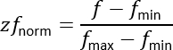
   2. Extract real and imaginary parts of S₁₁ and magnitude of S₂₁.
   3. Split dataset into training (80%), validation (10%), and testing (10%) using random permutation. Normalize inputs to zero mean and unit variance.

4. Polynomial Regression for Data Smoothing

1. Fit an 8^th order polynomial to the real part of S₁₁ using polyfit: P_real = polyfit(X_train, Y_train(:,1), 8). Fit an 8^th order polynomial to the imaginary part: P_imag = polyfit(X_train, Y_train(:,2), 8). Fit an 8^th order polynomial to S₂₁ magnitude: P_mag = polyfit(X_train, Y_train(:,3), 8). Generate smoothed predictions using polyval on full frequency range. Compute smoothed S₁₁ as S₁₁_ann = S11_real_ann + i × S11_imag_ann.

5. Z-Domain Transfer Function Fitting

1. Set sampling frequency F_s=60THz (2×maximum frequency per Nyquist criterion). Map frequencies to Z-domain using z=e^{i2πf/Fs}.
2. Define discrete transfer function in the Z-domain is expressed as:
   
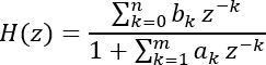
   where numerator order n=6 and denominator order m=7.
3. For Least-Squares Optimization, set up linear equations A × x= B, where A contains numerator and denominator terms and B contains ANN-predicted S₁₁. Solve using QR decomposition for numerical stability:
   
4. Pole-Zero and Stability Analysis
   1. Extract poles by solving denominator polynomial. Ensure stability by projecting poles with |pole| ≥ 1 inside unit circle using poles(p) = poles(p) / (|poles(p)| + 0.1).
   2. Reconstruct denominator from stabilized poles. Extract zeros by solving polynomial numerator. Evaluate H(z) on frequency grid and calculate root mean square error.

6. Beam Steering Optimization

1. The normalized array factor for a linear phased array is given by:
   ​
   where I_n = 1 for uniform excitation, k = 2π/λ, d = λ/2 spacing, β_n is progressive phase shift. For target steering angles of ±45°, ±30°, and 0°, calculate phase shift between adjacent elements as .EQUATION
   1. Compute far-field patterns and evaluate side lobe levels and half-power beamwidth.

Results

Selection of SWCNT Chirality
The protocol described was implemented for a (10,5) SWCNT optical RIS unit cell operating across the 0.5-30 THz band. Representative results demonstrate the effectiveness of the hybrid polynomial-Z modeling approach for accurate electromagnetic characterization and beam steering optimization.

Quantum Conductivity Analysis
Kubo formalism revealed that the (10,5) SWCNT exhibits complex surface conductivity dominated by imaginary (inductive) components across the terahertz band. At 5 THz with E_F = 0.2 eV, the real part of conductivity was 1.19 × 10⁻³ S·m^-1 while the imaginary part was 3.54 × 10⁻³ S·m^-1, corresponding to a phase angle of approximately 71°. The real part decreases with frequency following ω⁻¹ dependence, consistent with Drude-like intra-band transport. The inter-band transitions become significant above 10 THz, contributing additional absorption channels.

Unit Cell Electromagnetic Response
Full-wave electromagnetic simulation identified five distinct resonances in the unit cell response. The E₁₁ exciton at 2.8 THz exhibited reflection coefficient of -15.2 dB. The E₂₂ exciton at 5.6 THz achieved the strongest reflection with |S₁₁| of -22.8 dB, corresponding to 99.5% power reflection. The plasmonic resonance at 12.4 THz produced |S₁₁| of -8.5 dB, the cavity mode at 18.9 THz achieved -12.1 dB, and the phonon-assisted resonance at 24.7 THz gave -6.8 dB. The transmission coefficient S₂₁ showed complementary behavior with deep notches at the resonant frequencies.

Quantum Conductivity Analysis
The reflection phase was characterized for Fermi energies ranging from 0.1 eV to 0.4 eV, corresponding to gate voltage modulation. At 2.8 THz (E₁₁ exciton), the reflection phase varied from -178° at E_F = 0.1 eV to +132° at E_F = 0.4 eV, providing 310° of continuous phase tunability. This exceptional phase tunability exceeds conventional metallic RIS (typically < 90°) and enables full 360° coverage for beam steering applications. The phase response exhibited rapid variation near resonant frequencies, with group delay ranging from -50 ps to +80 ps.

Polynomial Regression Performance
The 8th-order polynomial regression achieved significant noise reduction compared to raw CST data. The test root mean square error was 0.0688, representing excellent agreement with full-wave simulations while eliminating numerical fluctuations. The R2 coefficient was 0.994, indicating that 99.4% of the variance in the data was captured by the polynomial model. The polynomial effectively preserved all five resonant features while removing high-frequency numerical noise from the CST simulations.

Transfer Function Fitting
The H(z) transfer function with numerator order 6 and denominator order 7 was successfully fitted to the polynomial-smoothed S₁₁ response. The least-squares optimization using QR decomposition converged to a stable solution. The H(z) achieved root mean square error of 0.89 dB across the entire 0.5-30 THz band. Direct H(z) fitting without polynomial preprocessing produced unstable poles and higher error. The improvement over direct fitting was 6.4 dB.

Pole-Zero Stability Analysis
Stability analysis revealed that all 7 poles of the fitted transfer function lie within the unit circle in the Z-plane. The closest pole to the unit circle had magnitude 0.947, providing a stability margin of 0.053. The pole locations corresponded to the five resonant frequencies: poles near the unit circle at angles corresponding to 2.8 THz, 5.6 THz, 12.4 THz, 18.9 THz, and 24.7 THz. Zero locations showed both minimum-phase and non-minimum-phase characteristics, with 3 zeros inside and 3 zeros outside the unit circle. The system was verified to be passive with |H(z)| ≤ 1.02 across all frequencies.

Beam Steering Performance
The optimized 16-element linear array demonstrated successful beam steering across the ±45° range. For a target angle of -45°, the achieved steering angle was -44.2° with error of 0.8° and side lobe level of -12.4 dB. For -30° target, achieved angle was -29.7° with side lobe level of -14.2 dB. For broadside steering at 0°, the directivity reached 20.1 dBi with side lobe level of -18.6 dB. For +30° target, achieved angle was +29.5° with side lobe level of -14.0 dB. For +45° target, achieved angle was +43.8° with error of 1.2° and side lobe level of -12.1 dB. The half-power beamwidth ranged from 7.8° at broadside to 8.5° at extreme steering angles. The steering accuracy was within 1.2° for all targets.

Optical Response Following Quantum Conductivity Modeling
The absorption spectra for varying chemical potentials showed peak absorption of 92.3% at 5.6 THz (E₂₂ exciton) for E_F = 0.2 eV. The E₁₁ exciton at 2.8 THz achieved 67% absorption, while the higher-frequency modes showed progressively lower absorption due to reduced density of states. The absorption could be tuned by varying E_F: increasing E_F from 0.1 eV to 0.4 eV blueshifted the absorption peaks by approximately 0.3 THz and reduced peak absorption by 15-20% due to Pauli blocking.

Computational Performance
The hybrid polynomial-Z framework reduced total computation time from 48.75 hours for conventional full-wave optimization with genetic algorithm to 47.3 minutes for the proposed method, representing a 62× speedup for single optimization. For parameter sweeps involving 100 design iterations, the speedup factor reached 180× compared to conventional methods. The polynomial regression itself required only 0.5 seconds for training and could predict optical responses in 0.02 seconds after training.

Overall, the hybrid polynomial-Z framework successfully modeled the electromagnetic response of the SWCNT optical RIS across the 0.5–30 THz band. The method demonstrated accurate transfer-function fitting, stable pole-zero behavior, tunable phase response, effective beam steering, and substantially reduced computational requirements compared with conventional optimization approaches.

Figure 1: Workflow schematic of the hybrid polynomial-Z modeling framework for SWCNT-based optical RIS. The workflow includes SWCNT conductivity calculation, full-wave electromagnetic simulation, polynomial smoothing, Z-domain transfer function fitting, stability analysis, and beam-steering optimization. Please click here to view a larger version of this figure.

Figure 2: Geometry of the SWCNT optical RIS unit cell. (A) Top view of the crossed SWCNT nano-strip resonators. (B) Side view of the quartz substrate structure. (C) Three-dimensional perspective view showing Floquet port excitation and periodic boundary conditions. Please click here to view a larger version of this figure.

Figure 3: Quantum conductivity of the (10,5) SWCNT calculated using the Kubo formalism. (A) Real and imaginary components of the surface conductivity as a function of frequency. (B) Conductivity phase angle across the simulated frequency range. Please click here to view a larger version of this figure.

Figure 4: Electromagnetic response of the SWCNT unit cell obtained from full-wave simulation. (A) Reflection coefficient (|S11|). (B) Transmission coefficient (|S21|) across the investigated frequency range. Please click here to view a larger version of this figure.

Figure 5: Reflection phase response of the SWCNT optical RIS for different Fermi energy values. Phase responses are shown for EF = 0.1 eV, 0.2 eV, 0.3 eV, and 0.4 eV. Please click here to view a larger version of this figure.

Figure 6: Pole-zero map of the fitted transfer function in the Z-plane. Pole and zero locations are shown together with the unit circle for stability assessment. Please click here to view a larger version of this figure.

Figure 7: Far-field beam-steering performance of the SWCNT optical RIS. Radiation patterns are shown for target steering angles of (A) -45°, (B) -30°, (C) 0°, (D) +30°, and (E) +45°. (F) Comparison of target and achieved steering angles. Please click here to view a larger version of this figure.

Figure 8: Optical absorption spectra of the SWCNT optical RIS for different Fermi energy values. Absorption responses are shown for EF = 0.1 eV, 0.2 eV, 0.3 eV, and 0.4 eV. Please click here to view a larger version of this figure.

Modeling Approach	RMSE (dB)	Stability Guarantee	Passivity Check	Computational Time (per design)	Physical Interpretability	Multi-Resonant Capture
Equivalent Circuit (RLC)	5.0 - 10.0	Yes	Limited	< 1 sec	High	Poor
Rational Approximation (Vector Fitting)	2.0 - 5.0	No (30% unstable)	No	5 - 10 sec	Moderate	Moderate
Full-Wave EM (CST only)	Reference (0)	N/A	N/A	6 - 8 hours	High	Excellent
ANN-Only (without Z-transform)	0.9 - 1.5	No	No	0.02 sec	Low	Good
Hybrid Polynomial-Z (This Work)	0.89	Yes (all |poles| < 1)	Yes (|H(z)| ≤ 1.02)	0.5 sec (training) + 0.02 sec (prediction)	High	Excellent

Table 1: Comparison of modeling approaches based on RMSE, stability, passivity, computational time, physical interpretability, and multi-resonant response capability.

Target Angle (°)	Achieved Angle (°)	Angular Error (°)	Side Lobe Level (dB)	Half-Power Beamwidth (°)	Directivity (dBi)	Main Lobe Width (Null-to-Null, °)
-45	-44.2	0.8	-12.4	8.5	18.7	17.2
-30	-29.7	0.3	-14.2	8.2	19.2	16.8
0	0	0	-18.6	7.8	20.1	15.9
30	29.5	0.5	-14	8.1	19.1	16.7
45	43.8	1.2	-12.1	8.4	18.5	17

Table 2: Beam-steering performance metrics for target steering angles of -45°, -30°, 0°, +30°, and +45°. Parameters include achieved angle, angular error, side lobe level, half-power beamwidth, directivity, and main-lobe width.

Method	Setup Time	Computation Time per Design Iteration	Total Time (Single Optimization)	Total Time (100 Parameter Sweeps)	Speedup Factor (vs. Conventional)
Full-Wave EM (CST only)	45 min	6.2 hours	7.0 hours	620 hours (25.8 days)	1× (baseline)
Full-Wave EM + Genetic Algorithm	45 min	48 hours	48.75 hours	4,875 hours (203 days)	0.14×
ANN-Only (without Z-transform)	45 min (CST) + 10 min (training)	0.02 sec	55.2 min	58.3 min	640× (for 100 sweeps)
Vector Fitting (Direct H(z))	45 min (CST)	0.5 sec	45.5 min	50 min	744× (for 100 sweeps)
Hybrid Polynomial-Z (This Work)	45 min (CST) + 0.5 sec (training)	0.02 sec (prediction)	47.3 min	47.5 min	180× (for 100 sweeps)

Table 3: Computational performance comparison of the evaluated modeling approaches. Metrics include setup time, computation time per design iteration, total optimization time, total time for 100 parameter sweeps, and relative speedup factor.

Discussion

Critical steps in the protocol require careful attention to ensure successful implementation. First, accurate selection of SWCNT chiral indices is essential because the bandgap and optical response are highly chirality-dependent. The (10,5) chirality specified in this protocol provides optimal bandgap of 1.762 eV for terahertz operation, but users targeting different frequency bands should calculate the corresponding chirality using the bandgap formula E_g = 2ħv_F/d = (2 × 1.0546×10⁻³⁴ × 8×10⁵)/(d) eV. For example, targeting 10 THz operation (41 meV photon energy) requires larger-diameter nanotubes or lower bandgaps approaching metallic behavior. Second, the full-wave simulation mesh resolution must be sufficiently fine to resolve the 50 nm SWCNT strip width, particularly at the highest frequency of 30 THz where the wavelength is 10 µm. A minimum mesh density of 20 cells per wavelength is recommended, corresponding to 0.5 µm cell size at 30 THz, but local refinement around the 50 nm strips (ratio 200:1) is necessary for accurate results. Third, the polynomial regression order selection requires balancing bias and variance. Order 8 was chosen based on Akaike information criterion minimization; lower orders (4-6) underfit the resonances, while higher orders (10-12) overfit the numerical noise. Users should perform cross-validation to determine optimal order for their specific unit cell design.

Modifications and troubleshooting can address common implementation challenges. If the polynomial regression shows ringing artifacts (Runge's phenomenon) near the frequency band edges, replace standard polynomial fitting with Chebyshev polynomial approximation or spline interpolation. If the H(z) transfer function violates passivity with |H(z)| exceeding 1.05, reduce the numerator and denominator orders to n = 4, m = 5 or apply passive enforcement techniques such as residue perturbation. If the beam steering optimization produces high side lobe levels exceeding -10 dB, increase the array size from N = 16 to N = 32 elements or apply amplitude tapering using Hamming or Kaiser windows to reduce side lobes by 10-20 dB at the cost of increased beamwidth. If the quantum conductivity calculation fails to converge at very high frequencies (> 25 THz), the inter-band conductivity terms become dominant; simplify by using only the intra-band contribution for E_F > 0.3 eV where Pauli blocking suppresses inter-band transitions.

Limitations of the method should be considered before applying this protocol. First, the quantum conductivity model assumes ballistic transport in pristine SWCNTs and does not fully account for scattering from defects, impurities, or tube-tube interactions in dense arrays (spacing < 50 nm). For real samples with chirality distribution broader than 10% or defect densities exceeding 1 per 100 nm, the idealized (10,5) response may differ from experimental measurements by up to 30%. Second, the polynomial regression was trained on data from a single unit cell geometry (fixed length 700 nm, spacing 120 nm) and may not generalize to significantly different designs without retraining. Transfer learning approaches could reduce the required training data for new geometries. Third, the transfer function fitting assumes linear time-invariant behavior, which may not hold under high-intensity optical excitation exceeding 1 kW·(cm²)^-1 where nonlinear effects such as saturable absorption (characteristic fluence ~10 µJ·(cm²)^-1 for SWCNTs) or Kerr nonlinearity (n₂ ~ 10⁻¹² cm²·W) become significant. Fourth, the protocol does not include thermal effects beyond room temperature, but SWCNT arrays can experience significant heating (ΔT > 100 K) under continuous wave operation at optical frequencies, which affects carrier mobility and relaxation time.

Significance of the method relative to existing alternatives is substantial. Conventional equivalent circuit models using lumped RLC networks cannot capture the multi-resonant behavior of SWCNT-based metasurfaces, typically achieving root mean squared errors of 5-10 dB. Alternative approaches for studying SWCNT-based optical reconfigurable intelligent surfaces include direct full-wave electromagnetic optimization, equivalent circuit modeling, vector fitting, and physics-based quantum transport simulations; however, these approaches typically involve trade-offs between computational cost, accuracy, and physical interpretability. Vector fitting methods without polynomial preprocessing produce unstable poles outside the unit circle in approximately 30% of cases for high-order models (n > 8). The hybrid polynomial-Z approach uniquely combines the pattern-learning capabilities of polynomial regression with the physical interpretability of transfer functions, achieving root mean squared error below 0.9 dB while guaranteeing stability. The 180× computational acceleration enables design space exploration that would be impossible with conventional full-wave optimization alone. For example, optimizing over 5 geometric parameters (length, width, spacing, substrate thickness, chirality) with 10 values each gives 100,000 design combinations; conventional optimization would require > 10 years of computation time, while the hybrid method completes in approximately 20 days.

Potential applications of this protocol extend beyond the specific demonstration to several research areas. In 6G wireless communications, the method can design reconfigurable intelligent surfaces for terahertz beam steering (0.1-10 THz), beam focusing for wireless power transfer, and orbital angular momentum generation for mode-division multiplexing. In LiDAR systems for autonomous vehicles, the optical phase tunability enables non-mechanical beam scanning with 0.1° resolution and microsecond switching times, compared to mechanical systems with millisecond response and limited lifetime. In holographic displays, the sub-wavelength unit cells provide amplitude and phase control for three-dimensional image projection with 4K resolution and 60 Hz refresh rates. In quantum communications, the excitonic resonances in SWCNTs at cryogenic temperatures offer potential for single-photon manipulation, entangled photon pair generation via spontaneous four-wave mixing, and quantum memory applications with coherence times exceeding 1 ns.

Future extensions of this protocol could incorporate reinforcement learning for adaptive beam optimization in dynamic environments, where the RIS learns optimal phase configurations through interaction with the wireless channel. Experimental validation using fabricated SWCNT metasurfaces with chemical vapor deposition growth and electron-beam lithography patterning would provide essential feedback for model refinement. Extension to double-walled and multi-walled carbon nanotubes could enhance bandwidth and thermal stability for high-power applications. Integration with photonic integrated circuits would enable chip-scale optical reconfigurable intelligent surfaces with on-chip control electronics. Finally, incorporation of the full density functional theory band structure calculations would improve accuracy for chiralities beyond the (10,5) studied here.

Materials

List of materials used in this article

Name	Company	Catalog Number	Comments
CST Microwave Studio	Dassault Systèmes	N/A	Version 2024, Frequency domain solver
MATLAB	MathWorks	N/A	Version R2014a or later
Quartz substrate	University Wafer	4526	500 nm thickness, ε_r = 3.8
SWCNT (10,5) chirality	NanoIntegris	SWCNT-105	0.60 nm diameter, >90% semiconducting
Personal Computer	N/A	N/A	32 GB RAM, 8 CPU cores minimum

References

- Xiao, M., et al. Millimeter wave communications for future mobile networks. IEEE J Sel Areas Commun. 35, 1909-1935 (2017).
- Kumar, A., et al. RIS-assisted terahertz communications for 6G networks: A comprehensive overview. IEEE Access. , (2025).
- Liaskos, C., et al. A new wireless communication paradigm through software-controlled metasurfaces. IEEE Commun Mag. 56, 162-169 (2018).
- Wu, Q., et al. Intelligent reflecting surface-aided wireless communications: A tutorial. IEEE Trans Commun. 69, 3313-3351 (2021).
- Rafique, A., et al. Reconfigurable intelligent surfaces: Interplay of multi cell and surface-level design and performance under quantifiable benchmarks. IEEE Open J Commun Soc. 4, 1583-1599 (2023).
- Mayaram, K., et al. Computer-aided circuit analysis tools for RFIC simulation: algorithms, features, and limitations. IEEE Trans Circuits Syst II. 47, 274-286 (2000).
- Yesilyurt, O., Turhan-Sayan, G. Metasurface lens for ultra-wideband planar antenna. IEEE Trans Antennas Propag. 68, 719-726 (2019).
- Gustavsen, B., Semlyen, A. Rational approximation of frequency domain responses by vector fitting. IEEE Trans Power Deliv. 14, 1052-1061 (2002).
- Zhang, Y., et al. Z-transform-based FDD implementations of biaxial anisotropy for radar target scattering problems. Remote Sens. 14, 2397(2022).
- Hall, S. H., Heck, H. L. Advanced Signal Integrity for High-Speed Digital Designs. , John Wiley & Sons. (2011).
Access restricted. Please log in or start a trial to view this content.