Automated Urine Sediment Microscopic Image Analysis Using YOLOv10 with Chimpanzee Leader Election Optimization

Summary

The study proposes a model utilizing the UMID dataset to detect and classify urine cells, including Red Blood Cells, White Blood Cells, epithelial cells, crystals, and bacteria. Employing YOLOv10 with Chimpanzee Leader Election Optimization, it attains 84% mAP50 on a test subset, potentially decreasing manual microscopy workload in clinical urinalysis.

Abstract

To diagnose various urinary diseases, it is vital to accurately detect urine cells. This paper presents a novel approach for detecting and classifying urine cells using the YOLOv10 (You Only Look Once version 10) model integrated with the CLEO algorithm. YOLOv10, known for its superior performance in object detection, is combined with CLEO, a nature-inspired optimization algorithm. The model is trained on the Urine Microscopic Image Dataset (UMID), comprising various types of urine cell images. Multiple cell types have been classified, including bacteria, epithelial cells, RBCs, WBCs, crystals, and casts directly from microscopic images of urine samples. Results from rigorous testing show that YOLOv10 integrated with CLEO is a robust tool for analyzing urine sediments, achieving a mean Average Precision@50 (mAP50) of 84% and a recall of 90%. Hence, the proposed approach offers significant speed improvements and consistency as compared to traditional methods of urine sediment analysis. The framework can automatically analyze urine sediment images in real time with good detection performance and has the potential to assist computer-assisted clinical urinalysis, thereby reducing the workload of manual analysis and diagnosis.

Introduction

Kidney disease, urinary tract infections, metabolic disorders, and systemic abnormalities can be detected by urinalysis, which is a very important process of diagnosis^1,2. It is essential to examine the urine sediments under the microscope to identify miniature constituents such as Red Blood Cells (RBC), White Blood Cells (WBC), bacteria, fungi, casts, etc³. However, conventional manual analysis by optical microscopy is labor-intensive and depends on the skill of the technician and may lead to inter-observer variability and inconsistent diagnoses in busy clinical environments^4,5.

A targeted method is needed to address difficulties with the automated examination of urine samples. The impressive real-time performance of deep learning in object localization and classification in image analysis holds promise for medical imaging, especially in the realm of object detection algorithms, a prominent example being the You Only Look Once (YOLO) family of algorithms^6,7,8. Previous research using YOLO variants has faced problems with overlapping urine particles, morphology variations of urine particles, class imbalance, and poor performance accuracy in complicated conditions^3,9,10,11. Additionally, reliance on manually chosen hyperparameters in these YOLO-based systems may hinder model generalization and optimization.

YOLOv10 is a current model that improves feature extraction, computational efficiency, and inference speed for analyzing images in real-time¹². But its performance is dependent on finding an optimal set of parameters, which is a complex, non-linear optimization problem and can influence the stability of convergence and the accuracy of the detection. Hence, it is essential to apply an efficient optimization method to improve the performance of the approach in detecting microscopic urine sediments. This research work integrates the CLEO algorithm, inspired by chimpanzee social hierarchy, to optimize YOLOv10 parameters. CLEO excels at balancing exploration and exploitation while effectively navigating high-dimensional optimization challenges, thereby overcoming the local optima traps common to traditional methods^13,14. This adaptation is important for urine sediment analysis. In this application, the imaging conditions vary, as well as the shape and the texture of the particles. Under such conditions, it is required to provide stable detection performance. CLEO can be used in real-time clinical applications and can achieve faster convergence and better global search results than other commonly used optimization algorithms¹⁵.

The progress made in the analysis of urine cells using deep learning is covered here. In the early automated urine sediment analysis, traditional image processing techniques like thresholding and feature extraction were applied in combination with classifiers like SVM, k-NN, Decision Trees, and Random Forest algorithm^{16,17,18,19,20}. These techniques had moderate success, but performed poorly for overlapping cells, different lighting conditions, noise, and intricate sediment morphologies. Additionally, there was a considerable level of domain knowledge needed for the manual construction of features. The rise of deep learning, specifically Convolutional Neural Networks (CNNs), has greatly enhanced image analysis, with architectures like AlexNet and ResNet attaining improved classification accuracy²¹. But most CNN-based methods still focus on image-level classification instead of real-time detection and localization of many sediment particles in microscopy images.

The YOLO family of object detection frameworks has gained popularity in the medical image analysis field for their fast and accurate performance. YOLO based systems like YOLOv3, YOLOv5, and YOLOv8 demonstrated acceptable real-time performance and improved localization of the urine sediment components compared to techniques based on region proposals, such as Faster R-CNN and Mask R-CNN^14,15,22. Yet there are difficulties, including sensitivity to class imbalance and less accurate classification for small or similar particles, and the use of manually chosen training parameters. Recent findings indicate that combining the metaheuristic optimization techniques such as Particle Swarm Optimization (PSO)²³, Genetic Algorithms (GA)²⁴, Grey Wolf Optimization (GWO)²⁵, Whale Optimization Algorithms (WOA)²⁶ and Ant Colony Optimization (ACO)²⁷ with deep learning systems^{28,29,30,31,32,33} can improve the optimization of hyperparameters and enhance the efficacy of training. Nonetheless, these traditional optimization techniques can get stuck in a local optimum and fail to explore the solution space in a high-dimensional world, leading to an early convergence.

CLEO is a new metaheuristic optimization method based on the social behaviour of chimpanzees, which improves the exploration-exploitation balance and global optimization. It has been shown to perform better than the traditional algorithms by eliminating local minima and successfully traversing the solution space to solve complex problems, but has not yet been fully explored for application in biomedical object detection and urine sediment analysis. The existing urine sediment analysis frameworks have focused on either improving detection architecture or optimizing it independently and do not provide much insight into how they will affect the diagnostic performance of real-time urine sediment analysis.

In light of these gaps in the literature, this research combines CLEO with the YOLOv10 architecture, which is better for feature representation and real-time performance, to automate urine sediment microscopy analysis. The framework is designed to improve detection accuracy and robustness, and to be integrated into real-time urinalysis systems for clinical use, combining the benefits of YOLOv10's fast detection of objects with CLEO's adaptive optimization of hyperparameters.

The study proposes a novel approach combining YOLOv10 and CLEO optimization algorithms for automated microscopy analysis of urine sediments for real-time use. YOLOv10 was selected for implementation because it provides outstanding detection performance with superior accuracy, computational efficiency, and real-time inference capabilities, making it well-suited for automated urine sediment microscopic image analysis. It improves end-to-end detection efficiency, reduces post-processing, and achieves high performance for small and diverse objects. This framework employs a metaheuristic optimization procedure to improve model parameter optimization and detection robustness, unlike existing YOLO-based methods that only concentrate on architectural improvements. It aims to enhance the accuracy of object detection of urine sediment in different classes and enhance the efficiency of the inference in the clinical environment. The research hypothesizes that this integration will lead to improved accuracy of detection, greater convergence stability and higher computational efficiency, ultimately aiding laboratory professionals in minimizing manual workload and ensuring consistency and speed in urinalysis.

Protocol

The data used in this study came from a public research database of microscopic urine sediment images. During the study, no personal information identifying the patient was used. The commercially available elements associated with this protocol are listed in the Table of Materials.

Acquire and Prepare Dataset
Microscopic urine sediment images comprising RBCs, WBCs, epithelial cells, crystals, casts, bacteria, and yeast were obtained. All images were saved in PNG or JPEG format using consistent naming conventions. Blurry or poor-quality images containing incomplete sediment artifacts were eliminated. Bounding box annotation software was used for object-level annotation of urine sediment particles. Each sediment type was assigned a class number, and annotations were exported in YOLO format containing the class identifier, normalized center coordinates, bounding box width, and bounding box height. Annotation quality was validated manually by randomly selecting annotated images.

The dataset was randomly divided into three subsets consisting of 70% training data, 15% validation data, and 15% testing data. We used Python Scikit-learn train_test_split() function with stratified sampling to divide the dataset. Each subset maintained proportional representation of all sediment classes. Stratified random splitting was employed to minimize class disparity across dataset partitions. The class-wise distribution of images to urine sediment categories is illustrated in Table 1.

All microscopic images were resized to 640 × 640 pixels using bilinear interpolation with OpenCV. Pixel intensity values were normalized to the range [0,1]. Data augmentation was performed using horizontal flipping, vertical flipping, random rotation (±15°), brightness adjustment, and contrast adjustment during training. The preprocessed images were saved in separate training, validation, and testing folders.

System Configuration
The experimental environment was configured for deep learning-based urine sediment analysis. Python version 3.10, the PyTorch deep learning framework, and CUDA Toolkit version 12.1 for GPU acceleration were installed. Additional Python packages including OpenCV, NumPy, Pandas, Matplotlib, and Scikit-learn, were installed. The repository for YOLOv10 implementation was downloaded and configured prior to experimentation. Deterministic GPU computation was enabled where possible, and all package versions used during experimentation were recorded to support reproducibility.

YOLOv10-Based Urine Sediment Detection
A schematic diagram of YOLOv10 is shown in Figure 1. Pretrained YOLOv10 weights trained on the COCO dataset were loaded. The final detection layer was replaced with a custom output layer by replacing the default COCO class count with the urine sediment class count. An anchor-free detection configuration was implemented based on the YOLOv10 structure.

Training hyperparameters were initialized with a learning rate of 0.001, batch size of 16, 300 epochs, AdamW optimizer, and weight decay of 0.0005. Cosine annealing learning rate scheduling was applied, and early stopping with a patience value of 20 was enabled during training.

The training dataset was input into the YOLOv10 network to generate bounding box predictions and class probabilities. Localization loss, classification loss, confidence loss, and total loss were calculated during training. Model weights were updated using backpropagation and gradient descent optimization. Validation was performed after each epoch using the validation dataset.

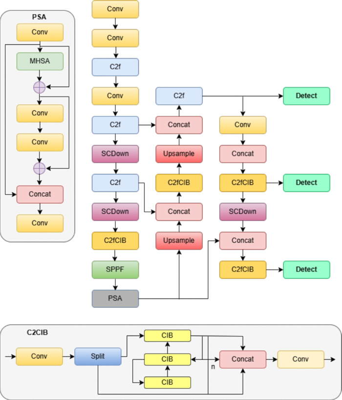
Figure 1: Architecture of YOLOv10. Schematic representation of the YOLOv10 object detection architecture used for automated urine sediment analysis. The figure illustrates the backbone, neck, and detection head components involved in feature extraction, multi-scale feature fusion, and anchor-free object detection for microscopic urine sediment particles. Please click here to view a larger version of this figure.

Chimpanzee Leader Election Optimization (CLEO)
A schematic diagram of CLEO is shown in Figure 2. The optimization search space included learning rate 0.0001–0.01, batch size 8–32, momentum 0.8–0.99, weight decay 0.0001–0.001, and confidence threshold 0.25–0.75. An initial chimpanzee population containing random candidate solutions was generated. YOLOv10 was trained using hyperparameters represented by each candidate chimpanzee, and model performance was evaluated using validation mean Average Precision (mAP). The fitness function was defined as:

Here,  , and represent weighting coefficients. The chimpanzee candidate with the highest fitness score was selected as the leader. The remaining candidate solutions were updated according to CLEO position updating rules. Exploration and exploitation processes were performed iteratively to identify optimal hyperparameters. The optimization process was repeated for 50 iterations or until the fitness improvement < 0.001. The weights assigned were  0.5,  0.25, and  0.25. The optimal CLEO-generated hyperparameters were applied to the YOLOv10 framework. The network was retrained using the complete training dataset, and the best-performing model weights were saved based on validation performance. The workflow of the proposed model is illustrated in Figure 3.

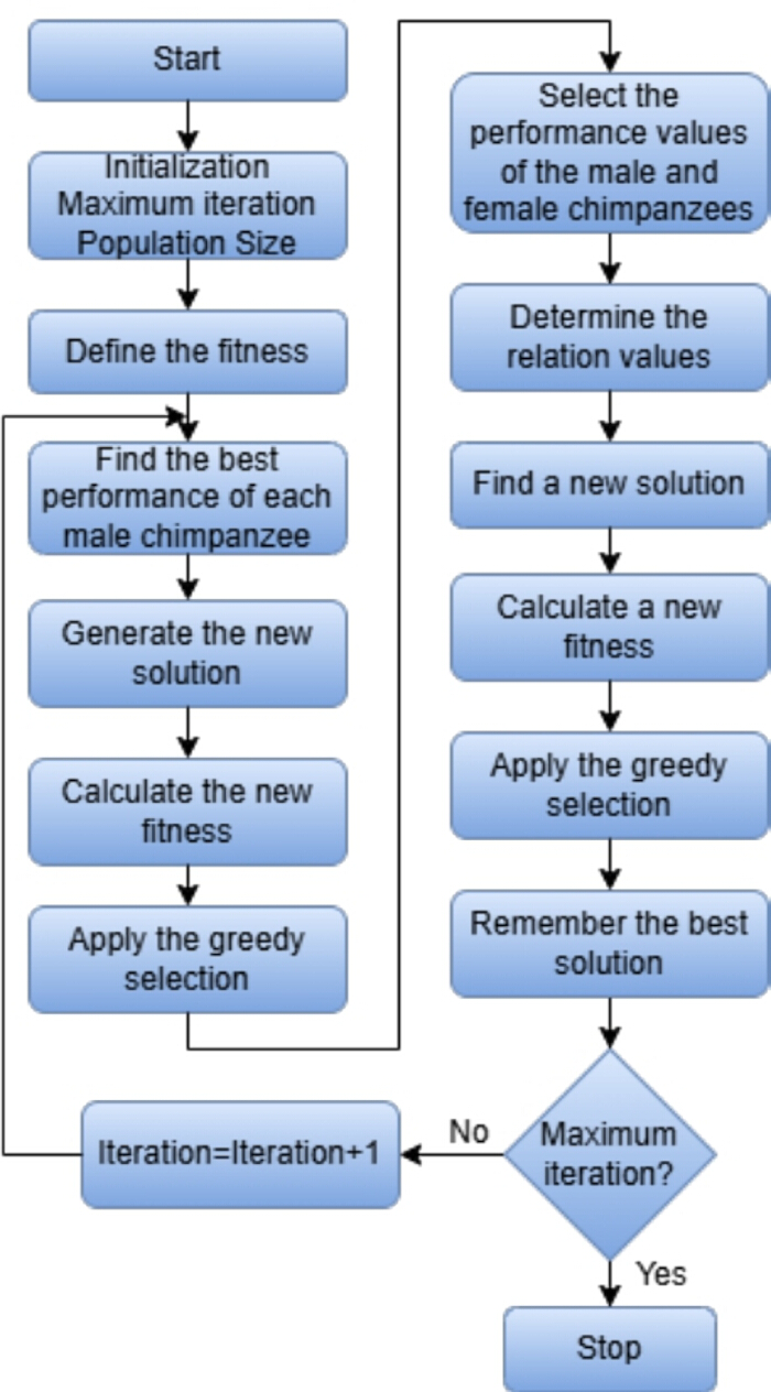
Figure 2: Chimpanzee Leader Election Optimization algorithm. Workflow of the CLEO optimization algorithm showing initialization of candidate solutions, fitness evaluation, leader selection, exploration-exploitation updating strategy, and iterative convergence for hyperparameter optimization of the YOLOv10 framework. Please click here to view a larger version of this figure.

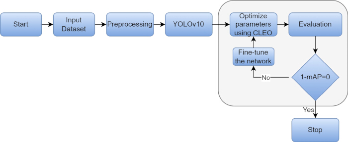
Figure 3: Workflow of the proposed model. Overall workflow of the proposed YOLOv10 + CLEO framework for automated urine sediment analysis, including dataset acquisition, image preprocessing, annotation, model training, CLEO-based hyperparameter optimization, detection, and performance evaluation. Please click here to view a larger version of this figure.

Model Evaluation
The optimized YOLOv10 + CLEO model was tested using the independent testing dataset. Performance evaluation metrics including accuracy, precision, recall, F1-score, mAP50, and mAP50-95, were calculated. Scikit-learn metrics functions were used for calculations. Average inference time per image was also recorded. Predicted sediment classes were compared with ground truth annotations to generate confusion matrices for all sediment categories. Frequently misclassified sediment particles were identified based on classification results. Comparison models including YOLOv5, YOLOv8, and Faster R-CNN were trained and evaluated using the UMID dataset under identical hardware configurations.

Results

The training and validation loss curves are shown in Figure 4, which depicts the YOLOv10 combined with CLEO performance metrics for urine cell detection. The accuracy of the predicted bounding boxes for detecting urine cells is measured by the box loss. The error in the prediction of the correct class is measured by the classification (cls) loss. The distributed focal loss (dfl) is used to improve bounding box regression accuracy. The values of all the training curves vary from 1.0 to approx...

Discussion

The results of this study provide compelling evidence of the potential of automated detection and classification of urine sediment components with the help of YOLOv10 and CLEO in the context of medical diagnostics. The proposed model provides a faster and more reliable solution for making timely decisions by optimizing YOLOv10 hyperparameters with CLEO. The proposed system provides high precision, recall, F1-score, and mAP values for various urine cells such as RBCs, WBCs, epithelial cells, bacteria, crystals and casts.<...

Materials

List of materials used in this article

Name	Company	Catalog Number	Comments
CUDA Toolkit 12.1	NVIDIA Corporation	Version 12.1/ RRID:SCR_018425	GPU acceleration platform
LabelImg Annotation Tool	Tzutalin	RRID:SCR_016189	Annotation tool
Matplotlib	Matplotlib Development Team	Version 3.x	Data visualization
NumPy	NumPy Developers	Version 1.x	Numerical computation
OpenCV	OpenCV.org	RRID:SCR_015881	Image pre-processing and analysis
Pandas	Pandas Development Team	Version 2.x	Data handling and analysis
Python 3.10	Python Software Foundation	RRID:SCR_008394	Programming language
PyTorch	PyTorch Foundation	RRID:SCR_018536	Deep learning framework
Scikit-learn	scikit-learn Developers	RRID:SCR_002577	Machine learning utilities
Ubuntu Linux	Canonical Ltd.	Version 22.04	Operating system
Urine Sediment Microscopic Dataset	Public dataset repository	GitHub - dipamgoswami/UMID-Urine-Microscopic-Image-Dataset: Urine Microscopic Image Dataset with point and box annotations · GitHub	Urine microscopy image dataset
YOLOv10 implementation	Ultralytics	YOLOv10: Real-Time End-to-End Object Detection | Ultralytics Docs	Object detection framework