Spatial Neighborhood Construction and NICHES Connectomics for Differential Ligand-Receptor Analysis in Fibrotic Human Lung

Summary

This protocol constructs radial spatial neighborhoods from imaging-based spatial transcriptomics data and applies NICHES ligand-receptor inference to build an edge-level connectomics graph. Using the fibrotic human lung as an example, it identifies, visualizes, and statistically compares inferred signaling between architecturally defined tissue neighborhoods.

Abstract

Spatial transcriptomics enables measurement of gene expression within intact tissue architecture, yet most analytical workflows emphasize cell-type classification over cellular interaction. Workflows that do infer intercellular signaling typically aggregate inferred interactions across clusters, regions, or spots, and fix neighborhood definitions, ligand-receptor (LR) databases, and scoring functions that users cannot easily inspect or change. The unmet need is therefore an analysis workflow that preserves signaling inference at the resolution of individual cell-cell pairs, constrains candidate interactions using measured physical distance, and exposes every modeling choice as a user-set parameter. Here, we describe a computational protocol that meets these requirements by inferring LR signaling at cell-cell pair resolution, grounded in physical tissue space, from imaging-based spatial transcriptomics data.

The workflow defines spatial neighborhoods and constructs a directed connectomics graph in which edges represent the set of inferred LR interactions between cells. Using the NICHES (Niche Interactions and Communication Heterogeneity in Extracellular Signaling) package, three complementary representations are derived: a Cell-to-Cell (C2C) edge-level connectome, a Cell-to-Neighborhood (C2N) outgoing signaling summary, and a Neighborhood-to-Cell (N2C) incoming signaling summary. A parallel Neighborhood Composition assay characterizes the local tissue architecture of the spatial neighborhoods. The framework is modular and tunable: users may adjust neighborhood definitions, select alternative LR databases, and modify scoring and aggregation methods. These node- and edge-aligned data layers support visualization, clustering, and differential analysis of spatially organized signaling patterns. Applied to fibrotic lung tissue, the workflow segregates architecturally defined neighborhoods and identifies differential LR mechanisms that distinguish fibrotic regions from surrounding tissue. This protocol provides a reproducible framework for studying spatially organized intercellular communication across tissues and disease contexts.

Introduction

The objective of this protocol is to provide a step-by-step, reproducible workflow for inferring LR signaling between individual, physically adjacent cells in spatial transcriptomics data and for statistically comparing that inferred signaling between architecturally defined tissue regions. We demonstrate a specific implementation in imaging-based data (10x Xenium) and discuss the parameter changes required to apply it to other spatial transcriptomics platforms. The workflow operates on any unit of analysis that carries a centroid coordinate and a transcript count vector, though an inferred LR edge describes two cells only when that unit is a single cell rather than a multi-cell spot.

Spatial transcriptomics technologies enable measurement of gene expression within intact tissue architecture, allowing cellular identity, architectural organization, and transcriptional programs to be analyzed in situ^1,2. Most analytical workflows begin by assigning cell types from gene expression profiles and projecting these labels onto tissue coordinates and low-dimensional embeddings such as Uniform Manifold Approximation and Projection (UMAP) or t-distributed stochastic neighbor embedding (t-SNE). This cell-type-centric approach provides a necessary spatial framework for interpretation, enabling visualization of where distinct cell populations reside and how transcriptional states distribute across tissue regions (Figure 1).

While effective for descriptive mapping, such analyses treat tissues primarily as collections of labeled cell populations, emphasizing which cells are present and where they are located, without directly resolving how they influence one another through local interactions. Moreover, gene expression-based annotations are inherently non-comprehensive: cells that are proximal in transcriptional space can be grouped together despite performing distinct functional roles, particularly when those roles arise from cell-cell signaling rather than transcriptional identity alone. As a result, important aspects of tissue organization and function may be obscured when analysis is limited to cell identity, location, and abundance.

A complementary framework, known as the cell-relation paradigm, instead emphasizes the roles cells occupy relative to one another as a fundamental unit of analysis for understanding how tissue organization arises³. Under this view, tissue structure and function emerge from context-dependent relationships, which are instantiated through coordinated signaling among neighboring cells. Disease-associated states can likewise emerge from alterations in these relational interaction rules, rather than solely from changes in cell identity, motivating the development of analytical approaches that address how cells communicate within tissue space.

Computational frameworks for LR inference from single-cell and spatial transcriptomics data have substantially advanced the study of intercellular communication by providing tractable approximations of relational signaling patterns^4,5,6. However, many existing workflows manage complexity by collapsing inferred interactions across clusters, regions, or spots. While effective for denoising and scalability, this strategy obscures relational structure at the level of individual cell-cell pairs and conflates heterogeneous interaction contexts. In addition, such workflows often encode implicit assumptions about neighborhood definitions, LR databases, and scoring functions that are difficult for users to inspect or adapt to specific biological questions⁷.

One principled way to preserve relational structure without collapsing information is to constrain the space of candidate interactions prior to inference. Defining spatial neighborhoods limits LR inference to physically plausible cell-cell pairs, thereby reducing the combinatorial search space while retaining single-cell resolution. Within these transparently defined neighborhoods, curated LR databases provide a mechanistic basis for annotating directed co-expression between cells, making differences in how cells send and receive signals explicit. In this way, LR inference provides an information-additive layer that augments gene expression-based cell identity with relational context, distinguishing functional heterogeneity even among cells with similar transcriptional profiles.

Together, these considerations define a set of design requirements for high-resolution relational analysis in spatial transcriptomics: preservation of cell-cell pair connectivity, constraint of candidate interactions using physical tissue context, and annotation of intercellular relations through directed, interpretable signaling mechanisms grounded in curated databases. Few existing frameworks integrate these elements within a unified, modular workflow that enables systematic exploration of relational structure across tissue space.

To address this gap, we present a spatial connectomics protocol centered on NICHES⁸, a framework that computes LR inference spatially at single-cell resolution. In this protocol, LR inference is grounded in measured cell centroids, and candidate signaling partners are defined using a spatial neighborhood rule. The neighborhood rule is itself a user-set parameter. Here we define local neighborhoods using a fixed spatial radius around each cell, such that cells within a specified distance are treated as potential interaction partners, and the resulting connectomics graph is visualized on the cells themselves (Figure 2). In contrast, a k-nearest-neighbor (kNN) rule, pairing each cell with its k closest neighbors irrespective of absolute distance, may be substituted where the user prefers. There are tradeoffs regarding either choice. A radius fixes the physical interaction scale but yields variable neighbor counts across regions of differing density, while kNN fixes neighbor count but allows the physical scale to vary. In lung tissue, where density differs sharply across alveolar septa and airspaces, we default to the radius so that the inferred interaction distance remains physically interpretable.

The NICHES pipeline then constructs a directed graph where each edge connects a sender-receiver cell pair within the neighborhood and carries scores for all LR mechanisms (Figure 3). While not shown graphically, autocrine edges are also included in the calculation. This construction is closely related to ε-neighborhood graphs from spatial graph theory, in which nodes are connected on the basis of a fixed distance threshold, but is extended here by assigning each edge a vector of molecular LR scores rather than a purely geometric weight, effectively forming “hyperedges” that capture the massively parallel nature of inferred LR signaling between cell pairs. This extension is independent of the neighborhood rule, since under the kNN option described above, the same molecular hyperedges are assigned to a k-nearest-neighbor graph rather than to an ε-neighborhood graph.

Beyond edge-level inference of cell-to-cell interactions (C2C), this protocol derives two complementary node-aligned summaries of inferred LR signaling. C2N profiles summarize the outgoing signaling profile of each cell by aggregating all directed edges originating at that cell, whereas N2C profiles summarize incoming signaling by aggregating all directed edges terminating at that central cell. In parallel, the Neighborhood Composition assay quantifies the cell-type composition of each cell's local neighborhood based on the same spatial neighborhood definition. Together, these layers enable integrated analysis of how LR signaling patterns, spatial context, and cell identity jointly shape tissue organization. Whereas C2C encodes LR signaling at the edge level between sender-receiver cell pairs, C2N, N2C, and Neighborhood Composition are node-aligned representations attached to individual cells and stored as aligned data frames (Figure 4).

A key strength of the workflow is its tunability across multiple stages of spatial LR inference. Users may adjust spatial neighborhood definitions, select alternative LR databases, modify signaling kernels, and alter data preprocessing choices. In this article, we present one concrete implementation of the framework, using a radial spatial neighborhood definition, a multiplicative LR scoring function, and LR inference performed on raw transcript counts. Raw counts preserve a direct “molecule × molecule” interpretation of LR scores but represent only one of several valid modeling choices. Parameter selection in spatial connectomics workflows depends highly on the biological question of interest and the associated analytical tradeoffs. Importantly, this implementation occupies a single option within a broader design space of possible connectomics inference strategies (Figure 5)⁹.

All steps of this workflow are implemented in reproducible R scripts that write intermediate checkpoint objects to disk, enabling an iterative walkthrough without re-computation of upstream processing steps. The accompanying scripts serve as an annotated reference tutorial implementation that users can adapt to their own datasets and analysis workflows. Documented updates to this workflow past publication may be found at https://github.com/RaredonLab/JoVE2026

Protocol

NOTE: This protocol uses publicly available, de-identified human spatial transcriptomics data from Gene Expression Omnibus (GEO) series GSE250346, generated with 10x Genomics Xenium (imaging-based, single-cell resolution) on a human lung tissue microarray (TMA), and does not involve new human subjects research¹⁰.

Computational requirements: The scripts do not request multiple cores and are not explicitly parallelized. One CPU core is sufficient, and at least 16 GB of RAM is recommended. On a Linux compute node, the full pipeline runs in approximately 50 min, roughly half of which is the initial data download. Runtimes may improve with future releases of NICHES.

1. Data Setup and Reproducibility (Scripts 00–01)

NOTE: This method establishes the computational environment and downloads a two-core spatial transcriptomics dataset representing control and fibrotic lung tissue.

1. Download and extract the supplementary code archive.
   1. Download the supplementary code archive (Supplemental File 1) and save it to a directory of choice.
   2. In terminal, navigate to the chosen directory and extract the downloaded archive by typing unzip followed by the file name.
   3. Type cd example_pipeline to enter the project directory. Confirm that R scripts (00_install_packages.R through 07_figures.R), config.R, and helpers.R are present.
2. Install required R packages
   1. Type mkdir -p logs, then hit enter to create a directory for logs. Then type Rscript 00_install_packages.R 2>&1 | tee logs/00_install.log in terminal to install all CRAN dependencies and the NICHES package (v1.2.1) from GitHub. The install script pins NICHES to commit c0abfbe0, which fixes the bundled copy of the FANTOM5 ligand-receptor database (curated as of April 2015).
   2. Verify that the terminal displays "All packages installed successfully!" with version numbers for packages.
3. Review the configuration file.
   1. Open config.R in a text editor to view all dataset-specific parameters: sample identifiers, coordinate column names, cell-type annotation column, analysis radius, and clustering parameters (Table 1).
   2. Confirm that cfg$samples$control is set to "VUHD090" and cfg$samples$fibrosis is set to "TILD049MA".
      NOTE: The two-sample design used here is not required by NICHES; single-sample or multi-sample designs are equally valid. Connectome complexity increases with cell number and will affect NICHES runtime and C2C edge data frame creation.
4. Download and subset the public dataset.
   1. Type Rscript 01_setup_data.R 2>&1 | tee logs/01_setup.log in terminal to download the processed Seurat object from GEO, subset to TMA5, extract the two configured cores, and build segmentation-capable plotting objects for downstream visualization tasks that utilize full segmentation rather than purely cell centroids.
   2. Confirm the terminal displays "Two-puck object: 27250 cells" and lists saved outputs. The script also downloads cell segmentation polygons to enable morphology-aware visualization.
      CAUTION: The segmentation download requires approximately 45 GB of free disk space and a high-bandwidth internet connection.
      NOTE: While not necessary for NICHES, segmentation polygons enable morphology-aware visualization; centroid-only visualization is sufficient for core inference. For spot based spatial workflows, visualization would then be modified to use centroid-based visualization.
5. Verify intermediate outputs.
   1. Confirm that intermediate/xenium_two_puck_processed.rds exists (27,250 cells across two cores).
   2. Confirm that intermediate/xenium_two_puck_counts_for_NICHES.rds exists with the RNA assay data layer set equal to raw counts, as NICHES requires unimputed transcript counts rather than normalized values.
   3. Confirm that intermediate/plotting_cores/ contains core_VUHD090_plotting.rds and core_TILD049MA_plotting.rds.
      PAUSE POINT: The workflow can be paused after step 1. Steps 2–6 require the intermediate objects generated here.

2. Radius Selection via ε-Neighborhood Graphs (Script 02)

NOTE: This method determines the spatial scale at which cell neighborhoods are constructed. The radius defines which cells are considered neighbors for downstream LR inference.

1. Run the candidate radius sweep.
   1. Type Rscript 02_radius_selection.R 2>&1 | tee logs/02_radius.log in terminal to evaluate candidate radii (10, 25, 35, 60 µm) on the fibrosis core, compute neighbor-count statistics, and generate ε-neighborhood graph visualizations centered on a focal cell.
   2. Confirm the terminal displays neighbor-count summaries for each radius (e.g., "r = 35 µm: mean = 25 neighbors, isolated = 0.1%").
2. Inspect the neighbor-count summary table.
   1. Open results/radius_sweep_summary.csv. Confirm that neighborhood density increases monotonically with radius and that the fraction of zero-neighbor (isolated) cells decreases.
   2. Identify radii where isolated cell fraction drops below an acceptable threshold (e.g., <1%) while mean neighbor count remains interpretable.
      NOTE: The specific radii range tested (10, 25, 35, 60 µm) were chosen based on typical cell sizes in human lung tissue and approximate size of mesoscale tissue structure. Other tissues may require different ranges. Adjust cfg$radius$sweep_um in config.R and rerun functions within Script 02 if the default radii are not appropriate for the dataset. In the fibrotic core, the isolated cell fraction is 19.5% at 10 µm, 1.0% at 25 µm, 0.1% at 35 µm, and 0.0% at 60 µm, so 10 µm is excluded on this criterion, and radii of 25 µm or larger are admissible.
3. Inspect ε-neighborhood graph overlays and select a working radius.
   1. Open figures/radius_sweep/ to review ε-neighborhood graph overlays generated for each tested radius.
   2. Assess each radius qualitatively: very small radii yield sparse, locally disconnected graphs that underrepresent neighborhood context; very large radii yield dense graphs that blur boundaries between distinct microenvironments.
   3. Select a working radius that captures contiguous local structure while preserving separation between tissue regions.
      NOTE: The optimal radius is tissue-dependent and reflects biological assumptions about the spatial scale of cell-cell signaling. The selection criteria (connectivity, interpretability, boundary preservation) generalize across tissues, but the specific radius value does not. In this workflow, 35 µm was selected and set in config.R, based on these criteria (Figure 6), with the ε-neighborhood graph density showing high interpretability of tissue structure from corresponding centroid density. At 35 µm, the median cell in the fibrotic core has 23 neighbors.
      Document and justify the chosen radius for the dataset, confirm that the conclusions hold across neighboring radii, and consider non-fixed radii implementations, such as kNN, if the biological question demands.
4. Confirm the saved radius selection object
   1. Verify that intermediate/radius_choice.rds exists, storing the selected radius and focal cell metadata for reproducibility.
      PAUSE POINT: The workflow can be paused after step 2. Steps 3–6 use intermediate/radius_choice.rds to apply the fixed radius.

3. Spatial LR Inference with NICHES (Script 03)

NOTE: This method executes NICHES to compute LR co-expression scores for all cell pairs within the selected neighborhood radius. NICHES produces two complementary output types: node-aligned assays (C2N, N2C) that summarize outgoing and incoming signaling per cell, and an edge-level connectome (C2C) that preserves the full resolution of directed cell-to-cell edges.

1. Confirm NICHES inputs.
   1. Verify that intermediate/xenium_two_puck_counts_for_NICHES.rds exists, containing raw transcript counts in the RNA assay data layer.
   2. Confirm that the object contains sample identifiers, centroid coordinates, and cell-type labels in the metadata columns specified in config.R.
2. Run NICHES to compute LR scores.
   1. Type Rscript 03_run_niches.R 2>&1 | tee logs/03_niches.log in terminal to execute NICHES independently on each tissue core using the selected radius and the FANTOM5 LR database (key modifiable parameters annotated in Figure 7).
   2. Confirm the terminal displays edge counts and LR mechanism counts for each core (e.g., "Control edges: 251302", "Fibrosis edges: 289232", "Common LR mechanisms: 47"), where the 47 mechanisms are the FANTOM5 pairs whose ligand and receptor genes are both present on the Xenium panel and detected in this dataset.
      NOTE: Typical runtime is under 3 min per core on a standard workstation. Larger datasets with more tissue microarray cores require longer.
3. Verify the node-level output object.
   1. Confirm that Script 03 saved the node-level object with C2N and N2C assays attached, each containing 47 LR mechanisms (rows) across 27,250 cells (columns).
4. Verify the edge-level C2C object.
   1. Confirm that intermediate/two_puck_C2C_rad35_raw_VUHD090_TILD049MA.rds exists, containing 47 LR mechanisms across 540,534 directed edges.
      NOTE: The C2C object must remain separate from the node-level object because its columns correspond to directed cell-cell edges, not individual cells. This edge-level representation is required for differential LR analysis in step 6. The distinction between node-aligned (C2N, N2C) and edge-aligned (C2C) representations is fundamental to this workflow. In this pipeline, node-aligned assays enable clustering and embedding alongside gene expression data; edge-aligned assays enable statistical comparison of inferred signaling patterns between tissue populations (Figure 3).
      PAUSE POINT: The size of the dataset can make NICHES inference computationally expensive. The workflow can be paused after Script 03 writes its intermediate RDS objects; downstream steps can proceed without re-computation.

4. Construction of the Neighborhood Composition Assay (Script 04)

NOTE: This method computes a complementary node-aligned representation that captures local cellular architecture rather than LR signaling. For each cell, the Neighborhood Composition assay records the counts and fractions of each cell type among its spatial neighbors.

1. Confirm the node-level NICHES object exists.
   1. Verify that intermediate/two_puck_NICHES_rad35_raw_VUHD090_TILD049MA.rds exists.
   2. Confirm the object contains centroid coordinates, sample labels, and cell-type annotations which are required to identify neighbors and count their cell types.
2. Build Neighborhood Composition assays.
   1. Type Rscript 04_neighborhood_composition.R 2>&1 | tee logs/04_neighcomp.log in terminal to compute, for each cell, the counts and fractions of neighboring cell types within the 35 µm radius.
   2. Confirm the terminal displays the number of cell types detected (e.g., "Cell types: 45") and saves the updated node-level object.
      ​NOTE: The Neighborhood Composition feature dimensions depend on the granularity of the cell-type annotation used. Finer annotations (e.g., 45 subtypes) yield higher-dimensional composition vectors; coarser annotations (e.g., 10 broad categories) yield lower-dimensional vectors. Select annotation granularity appropriate to the biological question.
3. Inspect the feature mapping table and assay dimensions.
   1. Open results/neighcomp_feature_mapping_finalCT_rad35.csv to verify that sanitized feature names map to original cell-type labels (e.g., "Activated-Fibrotic-Fibroblasts" maps to "Activated Fibrotic Fibroblasts").
   2. Confirm that the Neighborhood Composition assays have 45 features (one per cell type) and 27,250 columns (one per cell), matching the node-level object column dimensions.
      NOTE: The Neighborhood Composition assay is independent of NICHES and can be computed for any spatial transcriptomics dataset with cell-type annotations and centroid coordinates. It provides an architectural baseline against which signaling-based representations (C2N, N2C), gene expression, and edge-level spatial connectomics can be compared.
      PAUSE POINT: The workflow can be paused after step 4. Step 5 requires the neighborhood-augmented node object saved to intermediate/.

5. Dimensionality Reduction and Clustering of Node-Aligned Assays (Script 05)

NOTE: This method embeds and clusters each node-aligned assay independently to separate distinct tissue state structures. Clustering the Neighborhood Composition, C2N, and N2C assays separately enables direct comparison of how architectural context, outgoing signaling, and incoming signaling partition cells into groups.

1. Confirm the node-level object contains required assays.
   1. Verify that the node-level object contains the following assays: NeighComp_finalCT_rad35_rawcounts (Neighborhood Composition), C2N_rad35_raw (outgoing signaling), and N2C_rad35_raw (incoming signaling). If any assay is missing, rerun the corresponding upstream step before proceeding.
2. Embed and cluster each assay independently.
   1. Type Rscript 05_clustering.R 2>&1 | tee logs/05_clustering.log in terminal to process each assay through scaling, principal component analysis (PCA), UMAP embedding, neighbor graph construction, and Louvain clustering.
   2. Confirm the terminal displays cluster counts for each assay (e.g., "NeighComp: 17 clusters, C2N: 19 clusters, N2C: 11 clusters").
      NOTE: Clustering resolution is controlled by cfg$clustering$resolutions in config.R. The
      specific cluster counts depend on the dataset structure and the resolution parameter; they are not expected to match exactly across different datasets or computational environments.
      UMAP embeddings may also vary slightly across environments due to differences in
      random number generation and underlying package versions.
3. Review assay-specific UMAP and spatial projections.
   1. Inspect the UMAP plots in figures/umap/ to verify coherent cluster structure in each assay space.
   2. Inspect spatial projections in figures/spatial/ on both tissue cores. Confirm that Neighborhood Composition clusters correspond to spatially contiguous regions. Some histological motifs, such as venous, arteriolar, and conducting airway structures, should cluster depending on resolution.
      ​NOTE: Comparing visualizations across assays is a key analytical step. Cells in the same Neighborhood Composition cluster share architectural context (similar neighbors) but may differ in their signaling programs (different C2N or N2C clusters). Conversely, cells in the same signaling cluster may reside in architecturally distinct neighborhoods.
4. Select fibrosis-associated Neighborhood Composition cluster(s).
   1. Use the Neighborhood Composition spatial projection on the fibrosis core to identify cluster(s) corresponding to fibrotic foci or other microenvironments of interest.
   2. Record the selected cluster identifier(s) and set cfg$diffcomm$fibrotic_neighborhood_clusters in config.R before running step 6.
      NOTE: Focus cluster selection is hypothesis-driven. The choice depends on the biological question being addressed. Inspect spatial maps, cluster composition spectra, and domain knowledge to select clusters that correspond to the tissue zones of interest. In this workflow, cluster 5 was selected because it spatially localizes to a fibrotic focus region and is enriched for fibroblast-associated neighbor cell types (Figure 8). Underlying feature space analysis is key. For example, to understand the outgoing signaling profile of individual cells, examine spatial visualizations of the features underlying C2N signaling from a reference cell to its local neighborhood (Figure 9).
      PAUSE POINT: The workflow can be paused after step 5. Step 6 requires both the clustered node-level object and the edge-level C2C object.

6. Differential LR Analysis (Script 06)

NOTE: This method identifies LR mechanisms that are enriched or depleted within fibrotic focus neighborhoods compared to the surrounding tissue. The analysis operates on the edge-level C2C object, stratifying directed LR edges based on whether their sender and receiver cells both reside inside or outside the focus region defined in step 5. A cell-label permutation test provides robust identification of focus-specific inferred signaling patterns despite the non-independence of spatially connected edges (Figure 10).

1. Confirm focus cluster configuration.
   1. Open config.R and verify that cfg$diffcomm$fibrotic_neighborhood_clusters is set to the Neighborhood Composition cluster(s) selected in step 5.
2. Run differential LR testing.
   1. Type Rscript 06_differential_communication.R 2>&1 | tee logs/06_diffcomm.log in terminal. This script performs the following steps:
      1. Restrict edges to those within the fibrotic tissue core.
      2. Classify edges as Focus-Focus (both cells in the focus cluster) or NonFocus-NonFocus (both cells outside the focus cluster); edges with one endpoint in each are excluded.
      3. Compute observed effect sizes (difference in mean edge weight) for each LR mechanism.
      4. Perform a focus-label permutation test (500 permutations) to assess statistical significance.
      5. Apply Benjamini-Hochberg false discovery rate (FDR) correction¹¹.
         NOTE: Boundary edges are excluded from the contrast because such an edge belongs to neither arm of a two-group comparison, and assigning it to either arm draws that arm's mean toward the other. At 35 µm, these boundary edges number 14,254, which is 4.9% of all directed edges in the fibrotic core but 55.8% of edges touching a focus cell. Testing them as a third class is a biologically motivated extension and can be implemented by modifying the edge classes in Script 06.
   2. Confirm the terminal displays edge counts (e.g., "Focus-focus edges: 11,274",
      "NonFocus-NonFocus edges: 263,704") and the number of significant LRs.
      NOTE: NICHES generates one autocrine edge per cell, so these edges are present in the C2C object and are carried into the differential test. To exclude them, require that the sender and receiver cell identifiers differ when defining both edge classes in Script 06.Each permutation reassigns the focus and non-focus labels while keeping the spatial graph fixed, generating a null distribution for whether the observed enrichment is specific to the focus cluster or would arise from any random subset of the same size. Increasing the permutation count improves the precision of the p-value estimate at the cost of runtime.
3. Verify edge-class sizes.
   1. Open results/diffcomm/edge_class_counts.csv and confirm that both edge classes contain sufficient edges for stable testing.
4. Inspect differential results and select mechanisms of interest.
   1. Open results/diffcomm/permutation_results.csv to view all LR mechanisms ranked by effect size and FDR.
   2. Identify mechanisms that are significantly enriched (positive delta_mean, FDR < 0.05) or depleted (negative delta_mean, FDR < 0.05) within focus neighborhoods.
      NOTE: The effect size threshold, one standard deviation (SD), is a practical significance filter applied in addition to statistical significance. Adjust thresholds based on tolerance for false positives and the magnitude of effects relevant to the biological question.
5. Assess robustness by repeating the analysis at additional radii.
   1. Select radii in a range of interest and change the radius parameter in config.R.
   2. Rerun Scripts 02 and 03.
   3. Copy the clustered node object from the original run to the filename Script 06 expects at the new radius, so the focus cell set is carried over rather than re-derived.
   4. Run Script 06, repeating for each radius, and compare against the results at 25 and 60 µm tabulated in Table 2.
      PAUSE POINT: The workflow is complete after step 6. The exported tables and volcano plot (Figure 11) summarize differential LR results. Tissue-wide wiring visualizations (Figure 12) provide spatial context for selected mechanisms that passed thresholding.
      NOTE: To generate all publication figures, type Rscript 07_figures.R 2>&1 | tee logs/07_figures.log in the terminal. This script is provided as an aide for visualization purposes and uses cell identifiers hardcoded in config.R for reproducibility; update these identifiers for other datasets.

Results

Application of this protocol to a public human lung spatial transcriptomics dataset (GEO series GSE250346) yields reproducible and interpretable outputs across all stages of the workflow. Successful protocol execution is confirmed by an ε-neighborhood radius sweep that produces an interpretable spatial graph at the selected radius (Figure 6); node-aligned assay embeddings and spatial projections that separate architectural and signaling-defined tissue states (Figure 8); and differential LR mechanisms that distinguish fibrotic focus inferred signaling from surrounding tissue context within fibrosis cores (Figure 11).

Across the evaluated radii, mean neighbor counts increased from 2.2 at 10 µm to 13.5 at 25 µm, 25.0 at 35 µm, and 66.4 at 60 µm. At 35 µm, the ε-graph exhibited coherent local connectivity while preserving boundaries between distinct microenvironments, indicating successful neighborhood definition. In contrast, suboptimal radius selection produced characteristic failure modes. Radii below 25 µm yielded fragmented ε-graphs with sparse connectivity, limiting the capture of local tissue structure, whereas radii at or above 60 µm generated dense graphs in which boundaries between microenvironments are harder to resolve visually, although the differential ranking is unchanged at that radius. These outcomes define a practical range of neighborhood resolutions and provide a visual diagnostic for protocol success or failure.

To determine whether these results depend on the 35 µm neighborhood radius, the differential analysis was repeated with the spatial graph rebuilt at 25 µm and at 60 µm, holding the focus region fixed as the identical set of 1,104 cells identified at 35 µm so that only the neighborhood definition varied. Rebuilding the graph changed its size substantially, from 161,232 directed edges in the fibrotic core at 25 µm to 751,226 at 60 µm, yet the five mechanisms reported below remained the top five in the same order at every radius, and the rank correlation across all 47 mechanisms was 0.998 between 25 and 35 µm, 0.996 between 35 and 60 µm, and 0.993 between 25 and 60 µm (Table 2).

Execution of NICHES at the selected radius generated node-aligned and edge-aligned assays representing cell-cell inferred LR signaling at pairwise resolution. The two-core subset (27,250 cells total; 11,140 fibrotic and 16,110 control) yielded 47 LR mechanisms across C2N and N2C assays and 540,534 directed edges in the C2C object. These outputs enabled downstream embedding, clustering, and differential analysis of signaling programs. Inferred LR signaling is intrinsically sparse due to expression-level sparsity, multiplicative LR scoring, and constraints imposed by the gene panel and LR database. This sparsity is expected in biologically meaningful analyses. In contrast, sparsity caused by insufficient neighborhood connectivity reflects suboptimal execution, yielding reduced edge counts and poorly structured embeddings.

Neighborhood Composition analysis appended two node-aligned architectural assays to the node-level object: a raw neighbor-count assay and a neighbor-fraction assay. In this dataset, neighborhood composition was represented by 45 features corresponding to the unique cell-type labels present across the two tissue samples. Successful construction yielded structured neighborhood profiles that varied across tissue regions, whereas suboptimal runs would produce near-uniform compositions reflecting inadequate spatial resolution or over-smoothing.

Dimensionality reduction and clustering produced assay-specific embeddings and cluster assignments for Neighborhood Composition, C2N, and N2C, with corresponding spatial projections onto tissue coordinates (Figure 8). In the representative analysis, Neighborhood Composition clustering yielded 17 clusters, C2N yielded 19 clusters, and N2C yielded 11 clusters, showing distinct architectural and signaling states across assays. Suboptimal clustering outcomes were characterized by either excessive fragmentation into small, spatially incoherent clusters or collapse into a small number of broad clusters lacking spatial specificity.

Inflammatory fibroblasts are the strongest marker of Neighborhood Composition cluster 5 by a wide margin, present in the neighborhoods of 99% of cluster 5 cells versus 4% of cells outside the cluster, followed by CD8 T cells, mast cells, and venous endothelium (Figure 8C). Within the fibrotic core, 1,104 cells belong to this cluster, and these are the cells taken as the focus region. An inflammatory fibroblast-rich neighborhood is the architecture in which matrix deposition and adhesion signaling would be expected to dominate.

Differential LR analysis compared edge weights between two within-sample edge classes in the fibrosis core: Focus-Focus edges, in which both sender and receiver belonged to the selected Neighborhood Composition cluster(s), and NonFocus-NonFocus edges, in which both endpoints lay outside the focus. Results are summarized in results/diffcomm/permutation_results.csv, which ranks LR mechanisms by effect size and statistical significance using a cell-label permutation test (500 permutations).

Several LR pairs were significantly enriched within Focus-Focus edges, including VIM–CD44 (Δmean ≈ 3.46), FN1–ITGB1 (Δmean ≈ 1.97), FN1–CD44 (Δmean ≈ 1.70), COL1A2–ITGB1 (Δmean ≈ 1.23), and COL1A2–CD44 (Δmean ≈ 1.08) (Figure 12). These co-expression pairs reflect extracellular matrix (ECM)-integrin adhesion and matrix remodeling programs consistent with fibrotic microenvironments¹⁰. In contrast, MMP7–CD44 was lower within fibrotic foci (Δmean ≈ −0.52), below the effect-size threshold applied in Figure 11.

Differential results are visualized using a volcano plot (Figure 11), in which each point represents an LR mechanism. The x-axis indicates the difference in mean edge weight between Focus-Focus and NonFocus-NonFocus edge classes, and the y-axis shows −log10(FDR). Vertical dashed lines denote a practical significance threshold of approximately one standard deviation from zero. Suboptimal differential analyses were characterized by unstable effect size estimates and uniformly low statistical significance, producing volcano plots with broad dispersion near zero and no significant LR mechanisms after correction. These patterns indicate insufficient edge density or spatial signal, contrasting with the stable enrichment observed in successful protocol execution.

All analysis scripts, configuration files, and helper functions used to generate these results are publicly available at https://github.com/RaredonLab/JoVE2026.

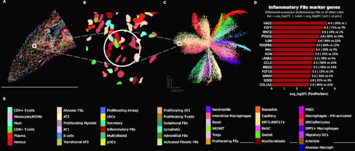
Figure 1: Cell-type-centric analysis of the gene expression assay. (A) Spatial cell-type map of a representative fibrotic tissue core (TILD049MA), with individual cells colored by assigned cell type and a reference cell indicated by a white circle. (B) Zoomed view of the circled region showing cell segmentations colored by cell type. (C) Uniform manifold approximation and projection (UMAP) embedding of all cells from both tissue cores, colored by cell type, with the reference cell indicated by a white circle. (D) Bar plot showing top marker genes for the reference cell's cell type (Inflammatory Fibroblasts), with bars indicating average log2 fold change from differential expression analysis (FindMarkers); labels show fold change and percent expression in cluster vs. other cells. (E) Color key legend for all annotated cell types. Please click here to view a larger version of this figure.

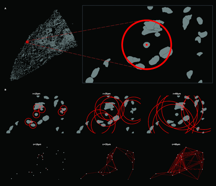
Figure 2: Construction of radial spatial neighborhoods and the resulting ε-neighborhood graph. (A) Full tissue view (left) with a reference cell marked by a red circle; zoomed inset (right) showing the local neighborhood around the reference cell (radius = 35 µm). (B) Top row: circular neighborhood overlays at increasing radii (r = 10, 35, 60 µm), done with a subset of cells to reduce visual overwhelm. Bottom row: corresponding ε-neighborhood graphs at each radius. Please click here to view a larger version of this figure.

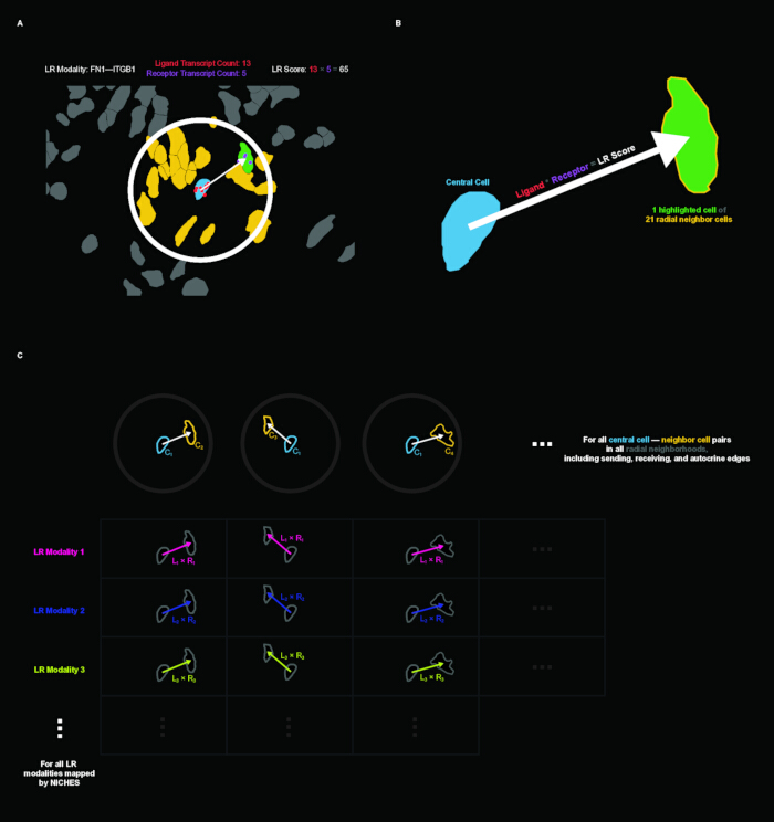
Figure 3: Ligand-receptor (LR) scoring and construction of the edge-level cell-to-cell (C2C) matrix. (A) Example of LR scoring in tissue context for the FN1–ITGB1 mechanism. A central cell (blue) sends to a neighboring cell (green) within the radial neighborhood; yellow cells are other neighbors. The LR score is computed as the product of ligand transcript count in the sender (13) and receptor transcript count in the receiver (5), yielding a score of 65. (B) Schematic illustration of directed cell-to-cell LR inference: a central cell sends an LR signal to one of its 21 radial neighbors. (C) Schematic of the C2C matrix structure. Columns represent directed cell-cell edges across all radial neighborhoods (including sending, receiving, and autocrine edges); rows represent LR modalities from NICHES inference. Please click here to view a larger version of this figure.

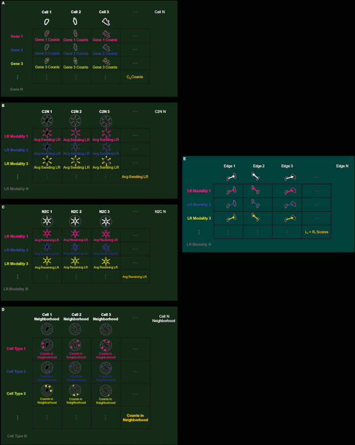
Figure 4: Schematic overview of the five primary data matrices. (A) Gene expression matrix: rows are genes, columns are cells, values are transcript counts. (B) C2N (Cell-to-Neighborhood) matrix: rows are LR modalities, columns are cells, values are average outgoing LR scores (node-aligned). (C) N2C (Neighborhood-to-Cell) matrix: rows are LR modalities, columns are cells, values are average incoming LR scores (node-aligned). (D) Neighborhood Composition matrix: rows are cell types, columns are cells, values are neighbor counts per cell type (node-aligned). (E) C2C (Cell-to-Cell) matrix: rows are LR modalities, columns are directed edges, values are individual L × R scores (edge-aligned). LR: Ligand-receptor. Please click here to view a larger version of this figure.

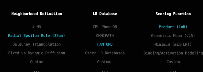
Figure 5: Three user-specifiable parameters of the connectomics inference workflow. Options for neighborhood definition, ligand-receptor database, and scoring function. Parameters used in this pipeline are highlighted in blue. Please click here to view a larger version of this figure.

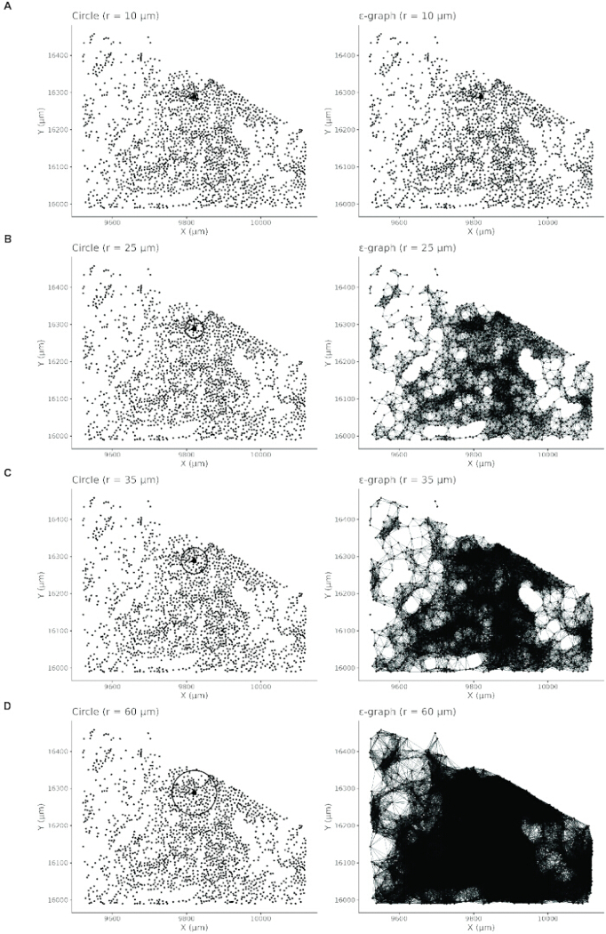
Figure 6: Paired visualization of circular neighborhood extent (left column) and corresponding ε-neighborhood graphs (right column) across four radius values. (A) r = 10 µm: neighborhoods are small, and the resulting graph is sparse with many isolated cells. (B) r = 25 µm: neighborhoods expand and graph connectivity increases. (C) r = 35 µm: neighborhoods capture local tissue structure with interpretable graph connectivity. (D) r = 60 µm: neighborhoods are large and the graph becomes overly dense, reducing interpretability. Please click here to view a larger version of this figure.

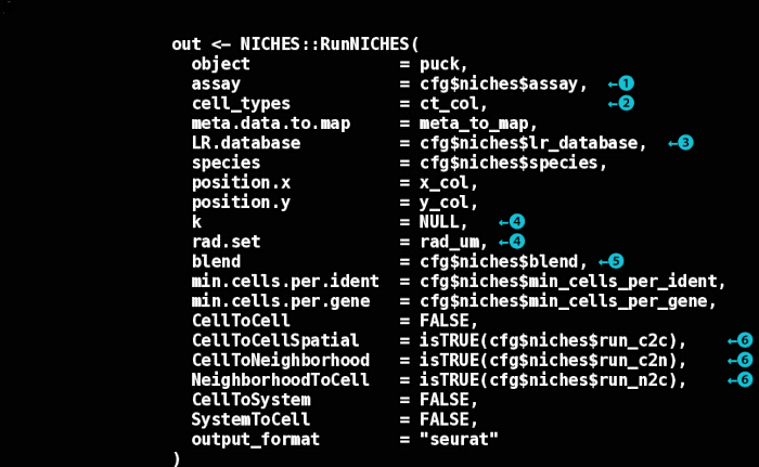
Figure 7: Annotated RunNICHES() function call. Key decision points are indicated by numbered circles. (1) Expression assay: which Seurat assay to use for LR quantification. (2) Cell type annotation: metadata column specifying cell identity for labeling LR vectors. (3) LR database: choice of curated LR interaction database. (4) Neighborhood definition: spatial neighborhoods defined by a fixed radius (rad.set) or k-nearest neighbors (k); setting one to NULL activates the other if defined. (5) Aggregation method: how neighbor signals are combined for node-level assays ("mean" or "sum"). (6) Output assays representations to compute: edge-level (CellToCellSpatial), outgoing node-level (CellToNeighborhood), and incoming node-level (NeighborhoodToCell). LR: Ligand-receptor. Please click here to view a larger version of this figure.

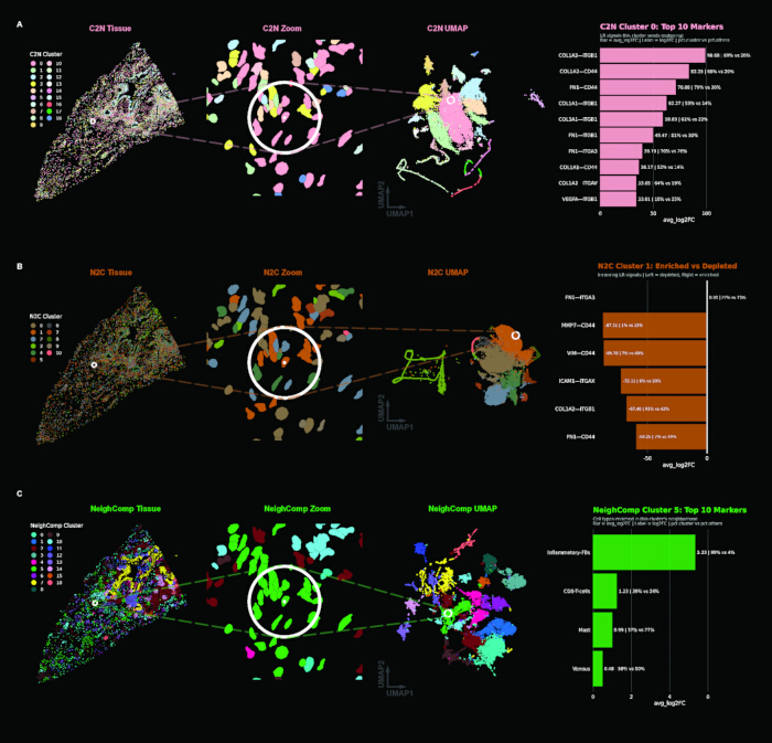
Figure 8: Clustering results for each node-aligned assay. (A) C2N (outgoing signaling): tissue view, zoomed region with reference cell highlighted, UMAP embedding, and spectral plot showing C2N Cluster 0 top markers. (B) N2C (incoming signaling): same layout with N2C Cluster 1 markers (FN1–ITGA3; the sparse spectrum reflects a generalized incoming signal profile and low feature space). (C) Neighborhood Composition (local architecture): same layout, with Neighborhood Composition Cluster 5 markers, where features are cell types rather than LR modalities. C2N: Cell-to-Neighborhood; N2C: Neighborhood-to-Cell; UMAP: Uniform Manifold Approximation and Projection. Please click here to view a larger version of this figure.

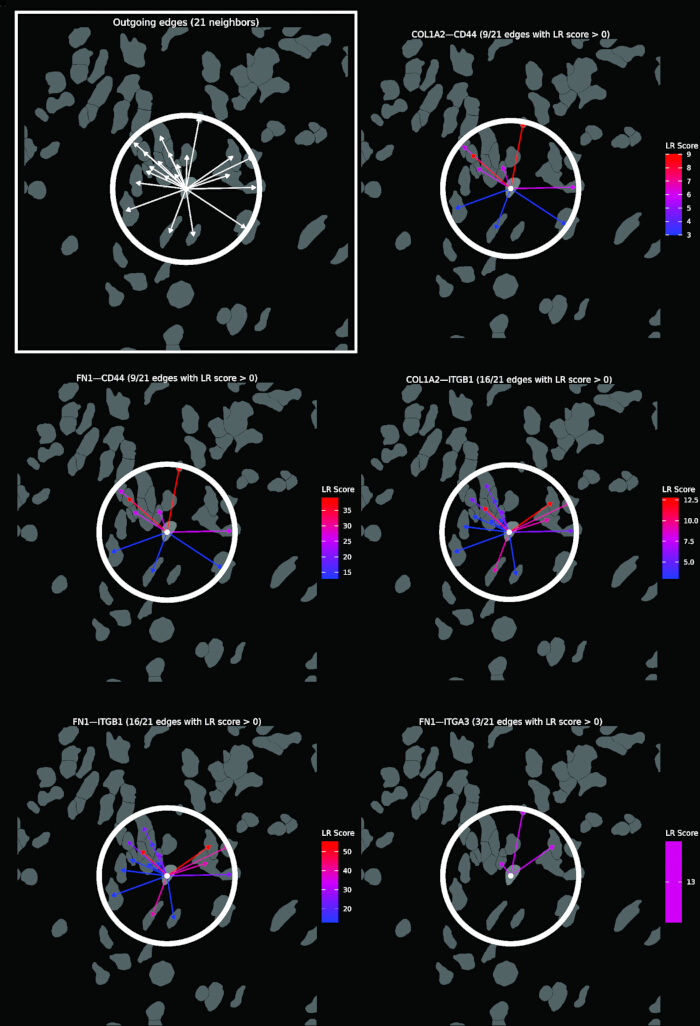
Figure 9: Visualization of outgoing C2N signaling from a single reference cell (white dot) to its 21 radial neighbors. The top-left panel (boxed) shows all outgoing edges as white arrows. The remaining panels show the same neighborhood decomposed by a selection of top LR mechanisms defining C2N Cluster 0. Arrows are colored by LR score (blue = low, red = high). C2N: Cell-to-Neighborhood; LR: Ligand-receptor. Please click here to view a larger version of this figure.

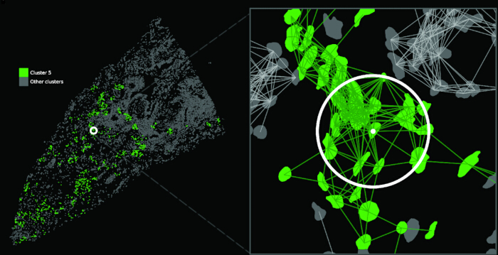
Figure 10: Definition of Focus-Focus and NonFocus-NonFocus edge classes. Left: Full tissue view with Neighborhood Composition Cluster 5 (fibrotic focus) shown in green and all other clusters in grey; a white circle marks the reference cell. Right: Zoomed view of the reference cell neighborhood with C2C edges overlaid. Green edges connect cells within Cluster 5 (Focus-Focus, intra-cluster); grey edges connect cells outside Cluster 5 (NonFocus-NonFocus, extra-cluster). C2C: Cell-to-Cell. Please click here to view a larger version of this figure.

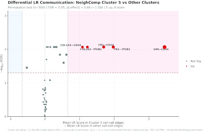
Figure 11: Differential ligand-receptor analysis between Focus-Focus and NonFocus-NonFocus edges. Volcano plot summarizing permutation-based differential LR analysis comparing Focus-Focus edges (both cells in Neighborhood Composition Cluster 5) against NonFocus-NonFocus edges. X-axis: difference in mean LR score (Cluster 5 edges - other edges). Y-axis: -log10 of the false discovery rate (FDR). Red dashed horizontal line: FDR = 0.05 significance threshold. Vertical dashed lines: effect size threshold (|Δ| > 0.66, approximately one standard deviation). Light red shaded region: enriched in fibrotic focus; light blue shaded region: depleted. Red points indicate LRs passing both thresholds (5 up, 0 down). Point size reflects effect magnitude. The footer describes the Y-axis calculation. LR: Ligand-receptor. Please click here to view a larger version of this figure.

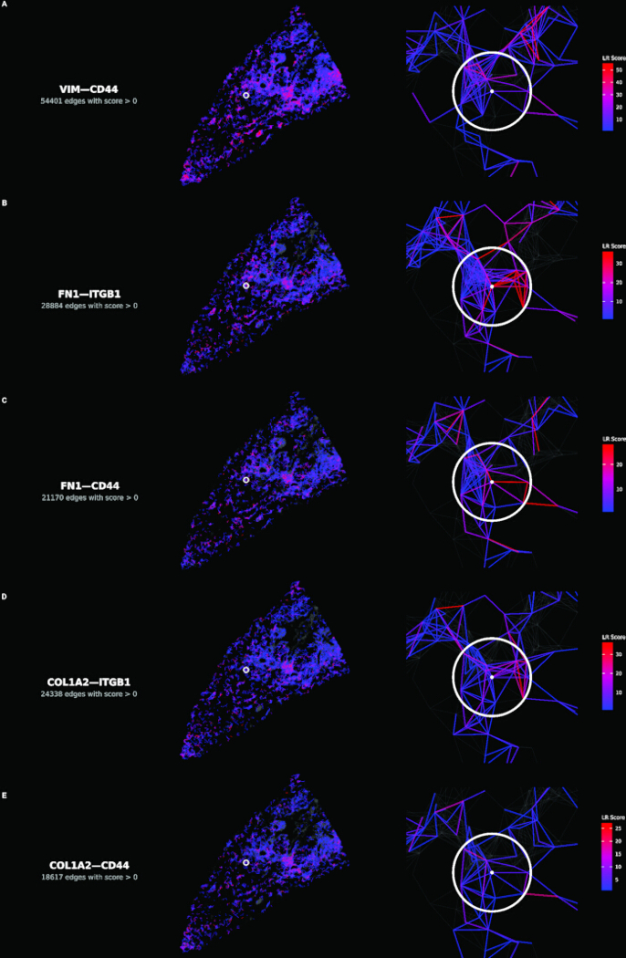
Figure 12: Spatial distribution of the five enriched ligand-receptor mechanisms. (A–E) Each row shows one mechanism, in descending order of effect size. Left panels: tissue-wide view with edges colored by LR score (blue = low, red = high); grey base shows inactive edges. Right panels: zoomed view centered on reference cell (white circle with center dot) showing local wiring architecture. LR score color scales are mechanism-specific. LR: Ligand-receptor. Please click here to view a larger version of this figure.

Table 1: Analysis parameters. Every parameter the workflow depends on, the value used in this implementation, where it is set in the configuration file or scripts, and whether the value is specific to this dataset. Please click here to download this file.

Table 2: Radius sensitivity. Edge counts and differential results with the spatial graph rebuilt at 25, 35, and 60 µm, holding the focus cell set fixed at the 1,104 cells identified at 35 µm. Effect sizes are the difference in mean LR score between Focus-Focus and NonFocus-NonFocus edges, with the rank of each mechanism in parentheses. Ligand-receptor. Spearman ρ between effect-size rankings across all 47 mechanisms: 0.998 (25 vs 35 µm), 0.996 (35 vs 60 µm), 0.993 (25 vs 60 µm). Please click here to download this file.

Supplementary File 1: Analysis code and configuration files. Please click here to download this file.

Discussion

The success of this workflow depends on several methodological choices that warrant careful consideration. Neighborhood radius selection fundamentally shapes the resolution of inferred signaling, and any neighborhood definition will fundamentally restrict the connectomics graph at the outset. The quantitative and visual diagnostics provided in step 2 support principled selection, but the optimal radius remains tissue-dependent and should be justified in the context of known cell sizes and signaling ranges for the system under study. The radius sensitivity analysis reported in the Results carries two qualifications. The edge sets are nested by construction, since every edge present at 25 µm is also present at larger radii, and per-edge scores do not depend on the radius, so the analysis measures the effect of admitting progressively more distant neighbors rather than of sampling an independent graph. The focus region was also held fixed by design, so the comparison isolates the effect of radius on the LR measurement rather than confounding it with a redefinition of the region. Edges are also not independent. At 35 µm, the 1,104 focus cells generate 11,274 Focus-Focus edges, roughly ten per cell, and because each edge score is a product of two cell-level values, edges sharing an endpoint share one of their factors and are correlated. The permutation test, therefore, randomizes cell labels rather than edge labels. Shuffling edge labels would narrow the null distribution and inflate significance. This does not remove the dependence between edges, but it prevents the test from being credited with more independent observations than the data contain. The two classes are also strongly imbalanced, 11,274 against 263,704 edges, which limits the precision of the Focus-Focus mean rather than biasing it. A single fixed radius also samples different amounts of tissue where cell density differs. At 35 µm, the mean neighbor count is 25.0 in the fibrotic core against 14.6 in the control, a 1.71-fold difference, and the coefficient of variation of neighbor counts is 56% higher in the fibrotic core. Because the neighborhood rule is user-specifiable, a density-adaptive radius or a k-nearest-neighbor definition can be substituted. Edge grouping is likewise user-specifiable, as edges can be grouped by any annotation carried on the edge object, such as cell-type pair or cluster assignment.

A distinctive feature of this workflow is its modularity. The spatial neighborhood definition, LR database, scoring function, and aggregation method are all user-specifiable, enabling adaptation to diverse biological questions without modifying core inference logic. The scripts provided are reference implementations tested only on the dataset used here and applying them to other data requires adapting data loading, metadata column names, and coordinate systems. FANTOM5 was selected for broad coverage of known signaling mechanisms; alternative databases such as CellPhoneDB or NicheNet can be specified in the NICHES call (https://github.com/msraredon/NICHES), and the intersection of panel with database should be considered at panel design. Dataset-specific content that this implementation relies on is confined to config.R (Table 1). The exception is the cell-type annotation, which cannot be abstracted away because Neighborhood Composition is built from those labels and inherits whatever scheme the source data carries. This modularity and transparency come with responsibility: users should document and justify their parameter choices, as different configurations can yield substantially different inferred signaling landscapes from the same underlying data.

Several limitations constrain interpretation. LR scores inferred from transcript abundance reflect signaling potential rather than protein-level activation or downstream pathway activity. Confirmation would require protein-level validation or functional evidence. Additionally, some LR pairs warrant particular caution, as not all pairs represent conventional secreted ligand-receptor signaling events. Vimentin is canonically an intracellular intermediate filament protein, so VIM-CD44 may constitute extracellular signaling only where vimentin is externalized, as can occur in inflammatory settings. Transcript abundance cannot establish whether that is the case here or whether the two proteins physically interact, so pairs such as these are best treated as hypotheses for validation rather than demonstrated interactions. Sparse transcript counts in spatial platforms can inflate zero-score edges, and product-based scoring may favor highly expressed genes. Segmentation error compounds this, since transcripts assigned to the wrong cell create ligand-receptor co-expression that was never present, and because misassignment is spatially local it falls preferentially on the short-range edges that carry the highest scores. Panel breadth bounds what is recoverable at all, since the 47 mechanisms tested here are the intersection of a targeted panel with FANTOM5. Edge-level matrices grow rapidly with cell number and neighborhood radius, which may constrain analyses of very large datasets without downsampling or batching strategies.

Relative to existing spatial communication methods, this workflow prioritizes edge-level mechanistic and spatial transparency. Unlike aggregation-based approaches that collapse signals across clusters or regions, the edge-aligned representation preserves directed cell-cell LR edges at full resolution, enabling hypothesis testing at the level of individual microenvironments. This granularity is particularly valuable when spatial heterogeneity is itself the object of study. Because these assays represent a different underlying feature space, their embeddings appear unlike those of gene expression data.

The general workflow can be applied to different spatial transcriptomics platforms, but what an edge represents depends on how the measurement is resolved to cells. On imaging-based platforms that assign transcripts to segmented cells, an edge connects two cells directly; these include 10x Genomics Xenium, Vizgen MERSCOPE, and Bruker CosMx. Sequencing-based data reach the same interpretation once the measurement has been resolved to cells, by segmentation and aggregation where the array element is smaller than a cell, as in Visium HD, or by deconvolution where it is larger, as on 10x Visium; where the unit remains a multi-cell spot, edges connect spots rather than cells and the analysis is interpretable at the level of regions rather than cell pairs. Imaging-based panels give cell-level resolution but bound the recoverable mechanisms to a targeted gene set, whereas sequencing-based platforms recover the transcriptome broadly but at units that must first be resolved to cells. As spatial transcriptomics platforms continue to mature in resolution and throughput, workflows that preserve cell-level relational structure while remaining interpretable and tunable will become increasingly valuable.

The workflow should extend naturally to emerging platforms. Both fixed-radius and kNN neighborhood rules generalize from a disk to a sphere in volumetric transcriptomics. Protein co-detection would also allow an edge to be scored on measured ligand and receptor abundance rather than the transcript alone. Additionally, LR databases that continually strengthen their empirical validation and attach metadata to each mechanism would give an edge to carry evidence quality or other annotations alongside their score. This protocol provides a foundation for such analyses, and the accompanying scripts offer an extensible starting point that users can adapt as the field develops new databases, scoring models, and integration strategies.

Materials

List of materials used in this article

Name	Company	Catalog Number	Comments
arrow	CRAN	version 16.1.0	Parquet/Feather file support (optional)
data.table	CRAN	version 1.15.4	Fast data manipulation
dbscan	CRAN	version 1.2.4	Fixed-radius nearest neighbor search
dplyr	CRAN	version 1.1.4	Data manipulation
ggforce	CRAN	version 0.4.2	Extended ggplot2 geoms (geom_circle)
ggplot2	CRAN	version 4.0.1	Data visualization
ggrepel	CRAN	version 0.9.5	Non-overlapping plot labels
Matrix	CRAN	version 1.7.0	Sparse matrix support
NICHES	GitHub (msraredon/NICHES)	version 1.2.1	Ligand-receptor communication inference
patchwork	CRAN	version 1.2.0	Plot composition
remotes	CRAN	version 2.5.0	GitHub package installation
scales	CRAN	version 1.3.0	Axis scales and formatting
Seurat	CRAN	version 5.4.0	Single-cell and spatial transcriptomics analysis
SeuratObject	CRAN	version 5.3.0	Data structures for single-cell data
sf	CRAN	version 1.0.16	Spatial polygon operations
tibble	CRAN	version 3.2.1	Data frame structures

References

- Stahl PL, Salmen F, Vickovic S, Lundmark A, Navarro JF, Magnusson J, et al. Visualization and analysis of gene expression in tissue sections by spatial transcriptomics. Science. 2016;353(6294):78-82.
- Rao A, Barkley D, Franca GS, Yanai I. Exploring tissue architecture using spatial transcriptomics. Nature. 2021;596(7871):211-20.
- Adler M, Chavan AR, Medzhitov R. Tissue Biology: In Search of a New Paradigm. Annu Rev Cell Dev Biol. 2023;39:67-89.
- Efremova M, Vento-Tormo M, Teichmann SA, Vento-Tormo R. CellPhoneDB: inferring cell-cell communication from combined expression of multi-subunit ligand-receptor complexes. Nat Protoc. 2020;15(4):1484-506.
- Jin S, Guerrero-Juarez CF, Zhang L, Chang I, Ramos R, Kuan CH, et al. Inference and analysis of cell-cell communication using CellChat. Nat Commun. 2021;12(1):1088.
- Dries R, Zhu Q, Dong R, Eng CL, Li H, Liu K, et al. Giotto: a toolbox for integrative analysis and visualization of spatial expression data. Genome Biol. 2021;22(1):78.
- Dimitrov D, Turei D, Garrido-Rodriguez M, Burmedi PL, Nagai JS, Boys C, et al. Comparison of methods and resources for cell-cell communication inference from single-cell RNA-Seq data. Nat Commun. 2022;13(1):3224.
- Raredon MSB, Yang J, Kothapalli N, Lewis W, Kaminski N, Niklason LE, et al. Comprehensive visualization of cell-cell interactions in single-cell and spatial transcriptomics with NICHES. Bioinformatics. 2023;39(1):btac775.
- Armingol E, Baghdassarian HM, Lewis NE. The diversification of methods for studying cell-cell interactions and communication. Nat Rev Genet. 2024;25(6):381-400.
- Vannan A, Lyu R, Williams AL, Negretti NM, Mee ED, Hirsh J, et al. Spatial transcriptomics identifies molecular niche dysregulation associated with distal lung remodeling in pulmonary fibrosis. Nat Genet. 2025;57(3):647-58.
- Benjamini Y, Hochberg Y. Controlling the False Discovery Rate: A Practical and Powerful Approach to Multiple Testing. Journal of the Royal Statistical Society: Series B (Methodological). 1995;57(1):289-300.
Reprints and Permissions
This article has been published
Video Coming Soon