Hybrid Deep Learning with Attention-Based Interpretability for PM2.5 Forecasting in Delhi Urban Environments

Summary

CORTA (Correlation Optimized Ranked Transfer-Attention)-Net, a hybrid deep learning framework for short-term PM₂.₅ forecasting in Delhi. The model combines CorrXGBoost-Rank feature selection, transfer learning with long short-term memory networks, and multi-head attention for temporal and feature-level interpretation and uses air-quality, meteorological, and satellite-derived fire-count data to improve PM_2.5 forecasting.

Abstract

Short-term PM_2.5 forecasting is challenging in Delhi because particulate matter concentrations are influenced by local emissions, meteorological variation, seasonal stagnation, and episodic fire-related pollution. This study presents CORTA-Net, a hybrid deep learning framework for PM_2.5 forecasting using multi-source environmental data from 2012 to 2024. The input data includes hourly air-quality observations from CPCB (Central Pollution Control Board) /DPCC (Delhi Pollution Control Committee) monitoring stations, meteorological variables from the India Meteorological Department (IMD), and satellite-derived fire-count information from MODIS (Moderate Resolution Imaging Spectroradiometer) products. The proposed framework first applies CorrXGBoost-Rank feature selection to reduce redundant predictors and retain important pollutants, meteorological, temporal, and fire-related variables. The selected features are then arranged as supervised sliding-window sequences and processed using a transfer-learning-based LSTM encoder followed by a multi-head attention layer. The attention mechanism provides feature- and time-step-level interpretation of the PM_2.5 forecast. CORTA-Net was evaluated using chronological training, testing, and validation partitions, as well as cross-validation. Compared with random forest, XGBoost, LSTM, and attention-LSTM baselines, the proposed framework reduced prediction error under the evaluated Delhi monitoring-station setting. The novelty of CORTA-Net lies in combining explicit CorrXGBoost-Rank feature screening, transfer-learning-based temporal encoding, MODIS fire-activity integration, and multi-head attention-based model-behavior analysis in a single reproducible PM_2.5 forecasting pipeline. Practically, the framework can support short-term urban air-quality forecasting in data-rich monitoring environments where pollutant records, meteorological observations, and fire-activity indicators are available.

Introduction

Fine particulate matter with aerodynamic diameter ≤ 2.5 µm (PM_2.5) is an important air-quality concern in Delhi because it is affected by local emissions^1,2,3, regional transport⁴, seasonal meteorology⁵, and episodic biomass-burning events⁶. During post-monsoon and winter periods⁷, low wind speed⁸, shallow boundary-layer conditions⁹, and temperature inversion can reduce pollutant dispersion and increase particulate accumulation. Forecasting of short-term PM_2.5 is challenging due to the inherent nonlinear, seasonal, and abrupt high-polluted phenomenon of the time series¹⁰. Previous studies on PM_2.5 forecasting have utilized statistical models, machine learning models, and recurrent neural network models¹¹. Statistical methods can be useful in determining trends and seasonality of data¹², but might not be able to fully account for the nonlinear interactions that exist between pollutants and meteorology¹³. Machine-learning models such as random forests and XGBoost can be used to model nonlinear relationships¹⁴; however, they typically do not have a temporal dependency unless lagged features are designed. Long short-term (LSTM) neural networks are capable of modeling both temporal dependency and nonlinear relationships¹⁵.

Long short-term memory networks can model temporal patterns¹⁶, but their performance may be affected by non-stationary conditions and abrupt pollution episodes¹⁷. Recent attention-based and transformer-based approaches improve temporal representation¹⁸, but many of them process all candidate variables directly and provide limited control over feature redundancy before sequence modeling^19,20. Although transformer-based and hybrid deep-learning models have recently improved PM_2.5 and AQI forecasting²¹, their contributions are often concentrated on temporal representation learning²², spatial graph construction²³, model fusion²⁴, or optimization. Many such models directly use the available multivariate input set and place the main learning burden on the sequence model²⁵. This can increase input redundancy, reduce interpretability, and make it difficult to identify whether improvements arise from temporal modeling, feature screening, external environmental indicators, or attention-based weighting. CORTA-Net is therefore positioned as a workflow-level forecasting framework rather than a new standalone neural-network layer²⁶. Its distinction lies in the ordered integration of four stages: CorrXGBoost-Rank feature screening before sequence modeling, transfer-learning LSTM encoding for temporal adaptation, MODIS-derived fire-count inclusion for episodic biomass-burning influence, and multi-head attention for feature- and time-step-level model-behavior interpretation. This design allows the framework to evaluate both forecasting accuracy and the contribution of selected pollutant, meteorological, temporal, and fire-activity variables under the same Delhi monitoring-station setting²⁷.

Recent advances in air-quality forecasting have increasingly used hybrid deep learning models, attention mechanisms, graph-based learning²⁸, and transformer architectures to capture nonlinear temporal and spatial dependencies²⁹. These approaches have improved forecasting performance by learning longer-range dependencies and assigning adaptive weights to time steps or input variables³⁰. However, many recent models still depend on large input feature sets, do not explicitly reduce redundant predictors before temporal modeling, or do not include external fire-activity indicators when episodic biomass-burning effects are important. CORTA-Net addresses this gap by combining feature screening, transfer-learning LSTM encoding, MODIS-derived fire-count integration, and multi-head attention in a single forecasting workflow.

This study presents CORTA-Net as a reproducible hybrid PM_2.5 forecasting pipeline rather than as a new neural network layer. The framework combines four stages: CorrXGBoost-Rank feature selection, transfer-learning-based LSTM temporal encoding, MODIS-derived fire-count integration, and multi-head attention-based model-behavior analysis. CorrXGBoost-Rank first reduces redundant pollutant and meteorological variables before sequence modeling. The selected features are then arranged into sliding-window sequences and processed using a transfer-learning LSTM encoder. MODIS fire-count variables are included as external indicators of regional fire activity, and the multi-head attention layer is used to examine which recent time steps and input variables contribute most strongly to the forecast. The framework is suitable for settings where continuous PM_2.5 observations are available from at least one monitoring station, preferably with several years of hourly data. It also benefits from meteorological observations and satellite-derived fire-count information when regional biomass-burning influence is relevant. Therefore, CORTA-Net is intended for data-rich urban air-quality forecasting settings and may not be suitable for locations with sparse, irregular, or short-term monitoring records.

Delhi was selected as the study region because it experiences recurring high PM₂.₅ levels during the post-monsoon and winter periods³¹. The city is affected by traffic, industrial activity, residential emissions, meteorological stagnation, and regional agricultural burning. Four monitoring stations were used for this study: Dwarka Sector 8, Anand Vihar, Mundka-DPCC, and Sonia Vihar. Each station represents a different type of urban microenvironment: residential area, traffic influence area, and area with industrial effects. The observations made from each monitoring station between 2012 and 2024 are presented in Supplementary Figure 1. Training of the model was done on data from 2015 to 2022, and testing was done on data from 2023 for both the model development and the model validation³² done on the data collected in 2024. The variables used as inputs included PM_2.5, PM₁₀, NO, NO₂, NOx, CO, benzene, temperature of air, wind speed, solar radiation, and barometric pressure, and were determined from what was available at the site³³. The MODIS-derived fire-count data were used as an external variable representative of the level of fire activity in the area. Table 1 contains a summary of the PM₂.₅ concentration statistics from each of the four monitoring stations.

Dataset	Station name	Mean	STD	min	25%	50%	75%	max
1	Dwarka Sector 8	98.24	79.12	7.52	38.65	70.83	133.47	588.15
2	Anand Vihar	115.87	89.42	8.91	49.28	84.36	152.89	574.92
3	Mundka-DPCC	113.62	91.05	4.21	43.58	86.74	158.42	682.31
4	Sonia Vihar	101.35	80.25	5.80	42.15	75.60	138.75	565.40

Table 1: Summary statistics of PM₂.₅ concentration at four Delhi monitoring stations. Table 1 presents average PM2.5 (fine particulate matter) levels measured at four monitors in Delhi. PM_2.5 consists of airborne contaminants smaller than 2.5 microns across, and as such, is small enough to be easily inhaled deeply into the lungs, thereby posing various potential health dangers.

Protocol

Methodology
A supervised sliding-window model was constructed to predict the future PM_2.5 value at time t + 1 from preceding hourly observations. Candidate input-window lengths of 12, 24, and 48 hourly time steps were evaluated using validation performance, and the final CORTA-Net configuration used a 24-hour input sequence. Linear interpolation was used to fill missing values; outliers were removed using the IQR method; and all variables were scaled using min-max normalization before generating lagged PM_2.5 features. The CorrXGBoost-Rank procedure was then applied for feature selection. First, Pearson correlation filtering retained variables with |r| ≥ 0.30. Second, highly redundant feature pairs with pairwise correlation |corr(x_i, x_j)| ≥ 0.85 were filtered to reduce multicollinearity. Third, an XGBoost regressor was trained on the remaining variables, and predictors with XGBoost gain-based importance scores ≥ 0.015 were retained for the final model input. The final CORTA-Net architecture consisted of stacked LSTM layers for temporal encoding, a multi-head attention layer for feature- and time-step-level weighting, and dense regression layers for PM_2.5 estimation. The model was trained using the Adam optimizer with mean squared error loss and early stopping. Model evaluation was performed using RMSE and R² across training, validation, testing, and 10-fold cross-validation partitions. Table 2 represents the Data preprocessing and feature engineering summary.

Step	Method used	Parameter / threshold	Purpose
Missing value calculation	Percentage of missing observations	Report variable-wise percentage	Quantifies data completeness
Short-gap imputation	Linear interpolation	Gap length ≤ 6 h	Fills short missing intervals
Outlier detection	IQR method	Q1 − 1.5 × IQR, Q3 + 1.5 × IQR	Removes invalid extreme values
Normalization	Min-Max scaling	Training-set min and max	Standardizes feature range
PM₂.₅ lags	Lagged variables	lag₁, lag₂, lag₃	Captures temporal persistence
Rolling statistics	Moving averages	3 h, 6 h, 12 h, 24 h	Captures short-term accumulation
Fire-count feature	MODIS FIRECOUNT	Same-day / previous-day count	Represents regional fire influence

Table 2: Data preprocessing and feature engineering summary. In Table 2, data processing is done in two ways: first, through the cleaning and transformation of the raw data (preprocessing), and second, via feature engineering to create/select/modify characteristics (features). As a unit, these two processes help eliminate or reduce noise; handle missing values; improve data consistency; and create more predictive models.

The normalization parameters were estimated only from the training set and then applied unchanged to the testing and validation sets to avoid information leakage.

Mathematical formulation of CorrXGBoost-rank
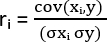
Let X = {x₁, x₂, ..., x_n} denote the set of candidate input variables, and y denote the target PM₂.₅ concentration. For each feature x_i, the Pearson correlation coefficient with the target variable was calculated as:

 (1)

where cov(x_i, y) is the covariance between feature x_i and target y, and σx_i and σy are their standard deviations. Retained features satisfying: |r_i| ≥ τ_r where τ_r = 0.30 in this study.

Pairwise correlations were calculated among all retained features_x_i, x_j, and if |corr(x_i, x_j)| >= τ_red, where τ_red = 0.85, the feature with the lower absolute correlation to the PM_2.5 target is dropped from the feature set. This process reduces variables from the feature set that have multicollinearity. Following this, an XGBoost regressor model was fit to the remaining features, and feature-importance scores were calculated for each feature using XGBoost importance, and features satisfying i_i ≥ τ_xgb where τ_xgb = 0.015 were kept in the final feature set (S") defined as S_final= S_corr ∪ S_xgb, i.e. the feature set defined by filtering features for redundancy with respect to correlation and removing any features based on XGBoost variable importance. The overall approach taken in the feature selection is as follows: calculate feature target pairwise Pearson correlation, discard features having |r_i|< 0.30, discard features with pairs having pairwise correlations ≥ 0.85, fit XGBoost to remaining features, keep features having XGBoost Importance Score ≥ 0.015, define the final desired features S_final=S_corr ∪ S_xgb, where S_corr are the features kept after redundant correlation filtering, and S_xgb are the features selected using XGBoost feature importance score. The CorrXGBoost-Rank workflow is therefore: compute feature-target Pearson correlation, remove features with |r_i| < 0.30, remove highly redundant features with pairwise correlation ≥ 0.85, train XGBoost on the remaining variables, retain variables with XGBoost importance score ≥ 0.015, and use the union of correlation-selected and XGBoost-selected variables as the final feature set. The parameters used in this study are τ_r = 0.30, τ_red = 0.85, and τ_xgb = 0.015.

Data sources
The authors integrated three large datasets for the study; these are data on air pollutants (PM_2.5, PM₁₀, NO₂, CO and SO₂) which the authors obtained through CPCB (Central Pollution Control Board) / DPCC (Delhi Pollution Control Committee) monitoring of air quality, meteorological data (temperature, humidity, wind speed/direction and pressure) from the Indian meteorological department (IMD) and satellite information on active fires from the MODIS Active Fire Products from NASA. These three datasets cover the 12-year period January 2012–December 2023 and thus represent different types of emissions. Fire incidents contribute to air pollution, as illustrated in Supplementary Figure 2, which shows FIRECOUNT trends from 2012 to 2024.

Long-term trends of pollutants across the study period
Figure 1 shows long-term trends of pollutants over the study years (2012–2024). Annual fire counts and average PM₂.₅ concentrations between 2012 and 2024 have a moderately strong positive relationship (r = 0.688), indicating that higher fire activity typically relates to higher PM₂.₅ concentrations. Both measured and predicted PM₂.₅ data follow a similar trend, supporting the idea that biomass burning contributes to particulate pollution. Although there is significant interannual variability, fire-related emissions are an important factor in determining PM₂.₅ variability, underscoring the need for regional fire management to improve air quality. The autocorrelation of predicted PM_2.5 at thirty lags, shown in Supplementary Figure 3, has considerable positive autocorrelation at nearly all thirty lags, confirming that PM_2.5 in Delhi has a strong temporal dependence and multi-day persistence.

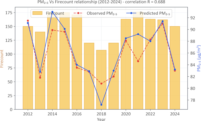
Figure 1: Long-term PM₂.₅ and fire-count trends from 2012 to 2024. Figure 1 compares annual fire-count variation with observed and predicted PM₂.₅ concentrations. PM₂.₅ is reported in µg/m³. FIRECOUNT represents satellite-derived fire activity from MODIS products. Please click here to view a larger version of this figure.

STL (Seasonal and Trend decomposition using Loess) decomposition
STL or Seasonal and Trend decomposition using Loess is an iterative algorithm that allows for the breakdown of time series data into three additive components as shown in Figure 2: trend (long-term trend) (Figure 2A), (Figure 2D), (Figure 2G), (Figure 2J), seasonal (cyclic periods) (Figure 2B), (Figure 2E), (Figure 2H), (Figure 2K), and remainder (noise/residual) (Figure 2C), (Figure 2F), (Figure 2I), (Figure 2L). STL has proven to be successful at dealing with the complex non-linear characteristics of environmental data (such as PM_2.5) for which many other analytical techniques have failed due to variable amplitudes in the seasonal signal and due to the existence of outliers. LOESS smoothing allows for accurate separation of these components, producing a clearer interpretation of trends or patterns. Through STL processing, it is possible to separate the broader upward PM_2.5 trends from the shorter daily/seasonal cycles and from the erratic residuals within those cycles. This separation allows for the identification of what emissions have influenced PM_2.5, as opposed to what meteorological factors have influenced PM_2.5. The results of this separation assist with accurate forecasting of future PM_2.5 emissions; provide data for regulatory decisions; and conform to the standards set out for rigorous disaggregation of time series data for air quality studies³⁴. Average daily PM_2.5 concentration measurements taken at monitoring stations in Delhi from 2012–2024 indicate minimal PM_2.5 level changes (i.e., no significant change from 2022–24) overall and extremely limited consistent behavior (or consistency in PM_2.5 levels among the four monitoring locations). The PM_2.5 levels at Dwarka Sector 8 and Mundka-DPCC are showing a persistent downward trend (i.e., continuing to decrease), while Anand Vihar has an increasing trend (i.e., increasing significantly), and Sonia Vihar has a slight upward trend (from a very small increase since 2022). In addition, the residuals of the daily PM_2.5 concentrations for each of the four monitoring stations indicated that PM_2.5 concentrations were strongly influenced by seasonal (meteorological) changes, which produced large fluctuations in the average daily PM_2.5 concentrations for individual stations. Daily PM_2.5 concentrations for the Four Monitoring Stations in Delhi (2012–2024) are displayed in Figure 2.

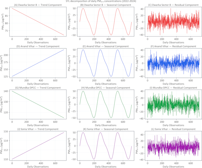
Figure 2: STL (Seasonal and Trend decomposition using Loess) decomposition of daily PM₂.₅ concentrations across four Delhi monitoring stations from 2022–2024. The time series for each monitoring station is decomposed into three additive components: long-term trend, seasonal variation, and residual (remainder). (A) Trend component for Dwarka Sector 8. (B) Seasonal component for Dwarka Sector 8. (C) Residual component for Dwarka Sector 8. (D) Trend component for Anand Vihar. (E) Seasonal component for Anand Vihar. (F) Residual component for Anand Vihar. (G) Trend component for Mundka-DPCC. (H) Seasonal component for Mundka-DPCC. (I) Residual component for Mundka-DPCC. (J) Trend component for Sonia Vihar. (K) Seasonal component for Sonia Vihar. (L) Residual component for Sonia Vihar. STL, Seasonal and Trend decomposition using Loess. Please click here to view a larger version of this figure.

Figure 2 presents the temporal decompositions of daily PM2.5 concentrations at four urban monitoring locations in 2022-2024, revealing patterns of long-term declines, gradual increases, and large diurnal changes. These differences can be largely attributed to the physical effects of weather, i.e., changes in the height of the planetary boundary layer (PBL), such as daytime expansion that increases vertical dispersion and lowers concentrations, and nighttime contraction, leaving pollutants close to the ground and creating a higher peak at night. Other meteorological influences come from local human activity emissions related to their hours of greatest volume (morning/evening peaks), industries, and their interactions with: site-specific factors, such as local topography, wind speed, relative humidity, and season (i.e. greater correlation in the winter) that create the station-specific changes and overall long-term declines may have been influenced by regulatory controls on emissions, leading to downward trends overall.

Correlation between the features
Figure 3 presents the distribution of all input features used in the CORTA-Net model. In panels, pollutant variables (PM₁₀ (Figure 3A), NO₂ (Figure 3B), CO (Figure 3C), SO₂ (Figure 3D)) show right-skewed distributions typical of urban air quality data, while O₃ (Figure 3E) and pressure (Figure 3I) exhibit near-normal patterns³⁵. Temperature (Figure 3F) displays a clear bimodal seasonal structure, humidity (Figure 3G) follows a broad uniform-like spread, and wind speed (Figure 3H) shows a light-tailed distribution. These patterns highlight the heterogeneous statistical behavior of the predictors and justify the need for feature engineering and normalization before model training.

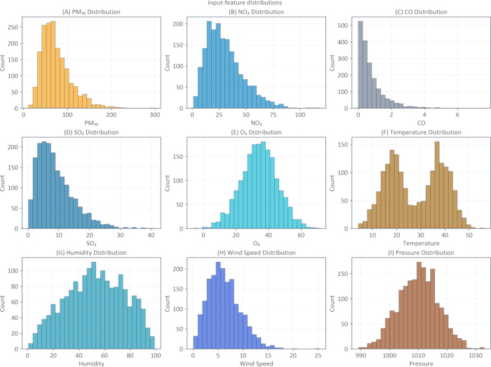
Figure 3: Distribution of input features used in the CORTA-Net model, including air pollutant concentrations and meteorological variables. The distributions illustrate the statistical characteristics of the predictors prior to preprocessing and model training. (A) PM₁₀ concentration. (B) NO₂ concentration. (C) CO concentration. (D) SO₂ concentration. (E) O₃ concentration. (F) Air temperature. (G) Relative humidity. (H) Wind speed. (I) Atmospheric pressure. Pollutant variables, particularly PM₁₀, NO₂, CO, and SO₂, exhibit right-skewed distributions typical of urban air quality data, whereas O₃ and atmospheric pressure show approximately normal distributions. Temperature displays a bimodal seasonal pattern, humidity has a broad distribution, and wind speed is concentrated at lower values with a light-tailed distribution. These heterogeneous feature distributions support the use of feature engineering and normalization before model development. Please click here to view a larger version of this figure.

Figure 4 presents the XGBoost gain-based feature-importance ranking after CorrXGBoost-Rank preprocessing for PM₂.₅ forecasting. The current feature-importance plot shows that Previous Day PM₂.₅ is the highest-ranked predictor with an importance score of 0.280, followed by PM₁₀ = 0.180, FIRECOUNT = 0.150, NO₂ = 0.120, CO = 0.080, wind speed = 0.070, temperature = 0.040, humidity = 0.030, and day of year = 0.020. The dashed vertical line represents the actual XGBoost feature-selection threshold of 0.015. Predictors with importance scores greater than or equal to 0.015 were retained for the final CORTA-Net input set, whereas predictors below this threshold, including SO₂ = 0.010, O₃ = 0.010, pressure = 0.005, rainfall = 0.005, weekend = 0.002, and holiday = 0.001, were excluded. These values represent XGBoost gain-based feature-importance scores and should not be interpreted as Pearson correlation coefficients or causal effects.

Therefore, only the features that received a contribution above this threshold were included in the model. XGBoost models use an ensemble of decision trees, which iteratively build a tree to minimize a loss function, known as gradient boosting. XGBoost calculates the importance of features using one of three metrics: gain (how much the split of the feature improves the model performance), weight (how many times the feature was chosen as a split for a tree), or cover (the number of observations impacted by the split). The XGBoost model was built upon data related to air quality (pollutants, meteorological variables) and has a focus on lagged PM_2.5 to auto-regressively forecast PM_2.5, which is common in PM_2.5 models for Delhi, and helps to capture the temporal persistence of PM_2.5. Delhi_PM_2.5 is a significant contributor due to the high autocorrelation characteristics of fine particulates, which also point to the presence of an inertia of pollution from the consistent emission sources. Wind Speed is a significant contributor because it provides the mechanism for the dispersion of the pollutants; whereas low winds allow for pollutants to build up during the winter when inversions are present. NO₂ is correlated with PM_2.5 due to the traffic/emissions, while the day of the year is an indication of the annual emission cycle of pollutants (i.e., lower emissions on the weekend). In Delhi, PM_2.5 has a high self-persistence due to the stagnant winter meteorology and continuous emissions from vehicles, industry, and biomass²⁸. Wind aids in the dispersion of aerosols, but weak wind < 2 m/s contributed to an increase in the build-up of PM_2.5 due to inversions. The relationship between NO₂ and PM_2.5 is a result of their common origin (i.e., combustion) and is subjected to temporal influences (e.g., daily vs. weekly)³⁶. The four primary factors responsible for explaining 93% or greater of the variation in AQI are variations in pollutant concentrations from lagged PM_2.5 accumulation (93%+) and low wind speeds trapping the emissions, the emissions of NO₂/PM from vehicles and industry, and day-to-day variations in the amount of traffic³⁷. In addition, the geography of Delhi is a contributing factor to the persistence of inversions in the area and thus also exacerbates PM_2.5 concentrations. Hyper-parameter tuning, regularization, and adding additional variables (such as temperature) would help limit the chances of over-fitting and would improve overall model performance. Implementing operational strategies to reduce PM emissions should include implementing daily limits on PM emissions, using devices that provide real-time monitoring for the presence of PM, and utilizing wind to disperse PM through the urban green space.

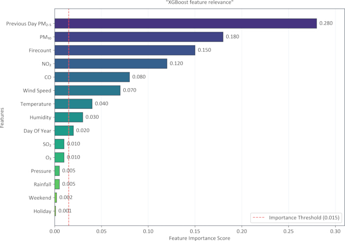
Figure 4: XGBoost gain-based feature-importance ranking after CorrXGBoost-Rank feature screening for PM₂.₅ forecasting. The predictor bars are arranged in descending order of importance. The dashed vertical line represents the actual XGBoost feature-selection threshold of 0.015. Predictors with scores ≥ 0.015 were retained for the final CORTA-Net input set, whereas predictors below this threshold were excluded. The ranking is used for feature screening and model-behavior interpretation and should not be interpreted as causal attribution. Please click here to view a larger version of this figure.

CORTA-net model architecture
Figure 5 presents a proposed PM_2.5 prediction framework. Supplementary Figures 4 and 5 illustrate the LSTM unit’s internal arrangement and a representation of the Multi-Head Attention block diagram. All data sources (i.e., ambient conditions, meteorological observations, fire activity, and both temporal and contextual aspects of data) underwent pre-processing to ensure that they agree temporally, have any missing data imputed (if necessary), and have been subjected to both outlier removal and normalization before employing them in any of the model-building processes. Model’s architecture, feature engineering, training configuration, data configuration, transfer learning, evaluation metrics, future predictions, and implementation details are shown in Supplementary Table 1. Utilizing the CorrXGBoost-Rank module, the optimal set of features is determined prior to a subset of these being input into the LSTM architecture, which has been enhanced by the incorporation of multi-head attention layers to account for time-series behavior during the modeling phase. Both the PM_2.5 forecast and PM_2.5 feature importance of the input features, as well as multi-head attention weights as attention maps, were provided as outputs. Internal LSTM unit structure and multi-head attention block diagram have been included as Supplementary Figures 4 and 5, respectively, while Supplementary Table 1 provides the architecture parameters for each layer type within this architecture.

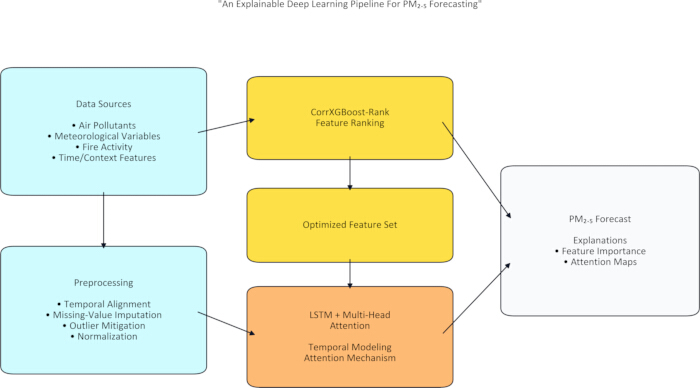
Figure 5: Overall architecture of the CORTA-Net PM₂.₅ forecasting model. An input forecast process includes inputs from air quality indicators, weather indicators, time indicators, and MODIS (Moderate Resolution Imaging Spectroradiometer) fire count indicators. For each of these steps, the algorithm aligned timestamps, handle missing values, filter outliers, normalize data, and engineer features. The final predictors were then selected using the CorrXGBoost-Rank process. Subsequently, the selected features were placed in time-sequence sliding windows and passed through an LSTM (Long Short-Term Memory) encoder using transfer learning. For each feature and time step, the multi-head attention mechanism applies weights before sending the combined output to the final regression dense layer to produce the PM₂.₅ prediction. Please click here to view a larger version of this figure.

Training and evaluation
A sliding-window approach was used to form supervised learning sequences. Training used Adam optimizer and mean squared error loss (Supplementary Table 2). Model performance was evaluated using RMSE and R² across training, validation, test, and cross-validation partitions. The Model’s architecture, feature engineering, Training Configuration, Data Configuration, Transfer Learning, Evaluation Metrics, Future Predictions, and Implementation Details are tabulated in Supplementary Table 1. Figure 6 represents the training diagnostics for the CORTA-Net PM₂.₅ prediction model. In panels, Figure 6A represents Training and validation loss curves, showing progressive error reduction, with optimal stopping at epoch 106. The evolution of the generalization gap during an evaluation of an over-fit analysis is illustrated by the divergence between validation and training data in Figure 6B. In particular, it shows periods where the divergence exceeds pre-defined limits; this information provides evidence that the learning-rate behavior and loss reduction patterns illustrate the benefits of scheduled learning-rate (LR) decay at critical epochs as a means of enhancing convergence stability as shown in Figure 6C. Collectively, these figures provide a summary of the learning dynamics, generalization capability and recommended training configuration of the model.

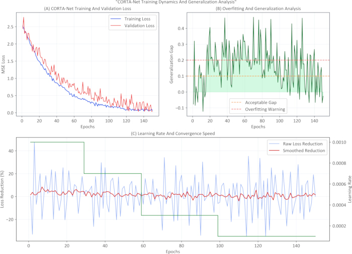
Figure 6: Training diagnostics for the CORTA-Net PM₂.₅ prediction model. (A) Training and validation loss curves showing progressive reduction in error during model training, with early stopping at epoch 106 based on validation performance. (B) Generalization gap between training and validation loss across epochs, illustrating the evolution of model generalization and periods of increased divergence indicative of potential overfitting. (C) Learning-rate schedule showing the effect of scheduled learning-rate decay on optimization throughout training. (D) Summary of model convergence behavior, demonstrating stable optimization and the final training configuration selected for the CORTA-Net model. Together, these diagnostics illustrate the model’s dynamics, convergence characteristics, and generalization performance during training. Please click here to view a larger version of this figure.

Results

Feature selection and forecasting results
The CorrXGBoost-Rank procedure selected lagged PM₂.₅, wind speed, humidity, temperature, temporal indicators, and MODIS-derived fire count as significant predictors of air quality. Each of these variables accounts for the persistence of pollution, dispersion due to meteorological conditions, seasonal differences in pollution levels, and regional influence from fires. Redundant variables were removed before sequence modeling to reduce unnecessary input dimensionality. CORTA-Net was evaluated using mean absolute error, root mean square error, and coefficient of determination. On the Delhi daily dataset, the model achieved RMSE = 3.19 and R² = 0.983. On the Daily Delhi Climate training partition, the model achieved RMSE = 4.98 and R² = 0.845. In the target test-set scatter analysis, observed and predicted PM₂.₅ values showed Pearson r = 0.942 and R² = 0.873. These values refer to different evaluation partitions and should not be treated as interchangeable model-wide results.

Figure 7 now serves as a single consolidated visual representation of the CORTA-Net testing performance on the test data. The time series section shows that there is an excellent correlation between actual and forecasted PM_2.5 level on the test data set throughout the evaluation time period, including episodic high pollution events like Diwali and crop residue burning events. In support of this, the scatter plot shows that there is a strong linear correlation between the actual and forecasted values (Pearson's r = 0.942, R² = 0.873), indicating an extremely high level of predictive accuracy.

Forecasting performance
The residual plots show that errors are roughly normally distributed around zero, with only a few isolated errors during extreme pollution spikes. This strongly supported the statistical robustness and absence of bias in the CORTA-Net models. CORTA-Net demonstrated an RMSE of 3.19 and an R² of 0.983 on the daily Delhi dataset and an RMSE of 4.98 and an R² of 0.844 on the Daily Delhi Climate Train dataset. These measurements, in conjunction with the above evidence, confirmed that CORTA-Net accurately modeled both gradual trends and sudden deviations in PM_2.5 levels.

The accuracy of predictions of PM_2.5 concentrations had been evaluated using three methods: a time-based evaluation of the time-validated accuracy of the models’ predictions of PM_2.5 concentration, a time-based correlation of the predicted and actual PM_2.5 concentrations, and an error assessment based on statistical analysis. The temporal evaluation, comparing PM_2.5 and temporal PM_2.5 predicted values (Figure 7A), showed the relationship over time of the actual measured PM_2.5 concentrations compared to the model-predicted PM_2.5 concentrations and demonstrates some significant PM_2.5 occurrences (e.g., the Diwali festival and stubble burning period) that occurred during this time period. The correlation between model-predicted PM_2.5 concentrations compared to measured PM_2.5 concentrations provides evidence of a very high correlation (Pearson r = 0.942 and R2 = 0.873), with a very strong agreement between predicted PM_2.5 concentrations and actual measured concentrations, indicating that the PP-FRC model is an accurate and reliable predictor of PM_2.5 concentrations (Figure 7B). The kurtosis distribution of the residuals (Figure 7C) demonstrated small errors over time with isolated high error days, while the residual distribution was approximately normal (Figure 7D), and the mean and median residual errors were very close to zero, indicating the model's prediction errors were unbiased and statistically well-behaved.

Figure 7: Predictive performance of the CORTA-Net model on the independent test dataset. PM₂.₅ concentrations are reported in µg/m³. (A) Temporal comparison of observed and predicted PM₂.₅ concentrations, demonstrating close agreement between measured and model-predicted values, including during major pollution episodes. (B) Scatter plot of predicted versus observed PM₂.₅ concentrations, showing strong predictive performance (Pearson r = 0.942; R² = 0.873). (C) Temporal distribution of residuals (prediction error) across the test period, indicating generally small errors with a limited number of high-error events. (D) Distribution of residuals, showing an approximately normal distribution centered near zero, with mean and median residuals close to zero, indicating unbiased and well-behaved prediction errors. Please click here to view a larger version of this figure.

Figure 7 presents the predictive performance of CORTA-Net on the target test set. The time-series plot showed the agreement between observed and predicted PM₂.₅ values, including periods of elevated particulate concentration. The scatter plot showed the association between predicted and observed PM_2.5 values. The residual plots showed that most prediction errors are centered near zero, with larger deviations during high-pollution episodes.

Cross-validation
Tenfold cross-validation showed limited variance across folds, demonstrating robustness under non-stationary atmospheric conditions. The model demonstrated strong predictive capability. Predicted PM₂.₅ values closely match observed values. Residuals showed minimal bias and approximate normality. Figure 8 provided an overview of the model's performance across many conditions and over time, using RMSE, MAE (mean absolute error), and R2 (coefficient of determination) measures in 10-way cross-validation. In panels Figure 8A and Figure 8B, RMSE and MAE were shown to exhibit low variability across all cross-verification training/validation gaps, indicating stable predictive accuracy. Panel Figure 8C shows consistently high R² values (~0.92 for training and ~0.89 for validation) across all cross validations, indicating that the model has high explanatory power and very low intra-model variance across the different cross validations. Figure 8D demonstrated that the mean value across all these measures showed little generalization gap, suggesting that the model consistently performed well regardless of how the data was partitioned.

Figure 8: Fold-wise performance of the CORTA-Net model using 10-fold cross-validation. Performance was evaluated using root mean square error (RMSE), mean absolute error (MAE), and coefficient of determination (R²). Error bars represent the standard deviation across folds where applicable. (A) Fold-wise RMSE values for the training and validation datasets, demonstrating consistently low prediction error across all folds. (B) Fold-wise MAE values for the training and validation datasets, indicating stable predictive performance with minimal variation between folds. (C) Fold-wise R² values for the training and validation datasets, showing consistently high explanatory power across all cross-validation folds. (D) Mean performance metrics and generalization gap between training and validation datasets, demonstrating consistent model performance and good generalization irrespective of data partitioning. Please click here to view a larger version of this figure.

Attention-based interpretability
Multi-head attention was used to examine which recent time steps and input variables contributed most strongly to the PM_2.5 forecast. Some attention heads emphasized short-term pollutant memory through lagged PM_2.5 values, while others assigned greater weight to meteorological variables related to dispersion, such as wind speed and humidity. Fire-count variables also received closer attention during pollution episodes consistent with regional biomass-burning influence. These attention maps should be interpreted as indicators of model behavior rather than causal explanations. The results suggested that the model uses both recent pollutant history and environmental covariates when producing forecasts.

Model configuration	Feature selection	Transfer learning	Multi-head attention	Fire-count input	RMSE ↓	MAE ↓	R² ↑
LSTM baseline	No	No	No	No	7.56	5.52	0.905
+ CorrXGBoost-Rank	Yes	No	No	No	4.24	3.10	0.970
+ Transfer learning	Yes	Yes	No	No	3.89	2.84	0.975
+ Multi-head attention	Yes	Yes	Yes	No	3.48	2.54	0.980
Full CORTA-Net	Yes	Yes	Yes	Yes	3.19	2.33	0.983

Table 3: Component-wise ablation analysis of CORTA-Net. Table 3 evaluates each architectural element within a system by removing or changing one or more components and measuring performance changes. This indicates which architectural components are most effective, confirms architectural decisions, and shows how the various components interact to enhance the accuracy, robustness, efficiency, and overall effectiveness of the network.

Table 3 presents the component-wise ablation analysis of CORTA-Net. The LSTM baseline obtained RMSE = 7.56, MAE = 5.52, and R² = 0.905. Adding the CorrXGBoost-Rank feature selection reduced the RMSE to 4.24, indicating that removing redundant and weakly relevant predictors improved forecasting performance. Transfer learning further reduced RMSE to 3.89, indicating that pre-trained temporal representations improved model stability. By using multi-head attention, the RMSE was lowered from 3.48 to 3.19, thus improving the R² value from 0.980 to 0.983, indicating a large improvement in temporal predictions through the use of feature and time step level weights in conjunction with the other components of the CORTA-Net model (i.e., CorrXGBoost-Rank, Transfer Learning, Multi-Head Attention, and MODIS Fire Count Inputs). Overall, the improvements demonstrated the contributions of feature selection, temporal transfer learning, attention-based sequence weighting, and fire activity to the implementation and performance of the CORTA-Net model.

Feature Selection	Temporal Sequence Modeling	Transfer Learning	Attention-based Model Behavior Analysis	Fire-activity Input	Main Role in Comparison
No explicit CorrXGBoost-Rank	No	No	No	No	Classical nonlinear machine learning baseline
Internal tree-based importance only	No	No	No	No	Gradient-boosting baseline for tabular predictors
No	Yes	No	No	No	Recurrent temporal baseline
No	Yes	No	Yes	No	Attention-based recurrent baseline
Yes	Yes	Yes	Yes	Yes	Proposed hybrid forecasting framework

Table 4: Key differences between CORTA-Net and baseline forecasting models. Table 4 shows that the current model used for forecasting is CORTA-Net, which allowed for more advanced techniques for extracting temporal features as well as using the ability to adaptively attend based upon what was important in order to capture complex temporal patterns from time-series data sets. CORTA-Net dynamically learnt how to relate many different scales of time to produce greater overall accuracy, robustness, and ability to create generalizations than traditional baseline forecasting techniques.

The differences between the CORTA-Net methodologies and the comparison baseline models are provided in Table 4. Random Forest and XGBoost can be used to provide a nonlinear machine-learning baseline method, but lack the direct modeling of sequential dependencies. LSTMs were used as a recurrent temporal baseline method, whereas Attention-LSTMs provided attention-based weighting without explicitly screening features, using transfer learning or integrating fire activity. In contrast, CORTA-Net incorporates four aspects of previous baselines into one forecasting pipeline: (1) CorrXGBoost-Rank feature selection; (2) transfer-learning LSTM encodings; (3) multiple-head attention; (4) and MODIS-derived fire count as input data.

Baseline comparison
In addition to quantitative baseline comparisons (provided separately with mean fold differences, standard errors, and 95% confidence intervals), the authors also assessed CORTA-Net’s internal functioning through its attention mechanism. Attention weights assigned to each input feature (over time steps and multiple attention heads) are shown in Figure 9. In Figure 9A, the group shows a representative distribution of attention weights assigned to one of the test dataset instances. As seen in this figure, although certain input features (e.g., PM2.5 at t-1, t-2, and t-3) would have lower relative weights than other predictors, they would still receive the highest attention/weights, demonstrating that CORTA-Net pays more attention to short-term temporal dependence than longer-term memory dependence. In Figure 9B, the researchers provide aggregate assessments of the relative importance of all input features across all the test samples in predicting PM_2.5 for Delhi; lagged PM_2.5, wind speed, temperature, and fire count are identified as the most important predictive input features. In Figure 9C, the authors demonstrate the multi-head attention patterns of CORTA-Net, where each head captures different, yet complementary, temporal and/or feature-level relationships among the input features, thus allowing it to learn a richer representation of the input features. In Figure 9D, the authors illustrate the time-stepping flow of attention, over time, with respect to PM₁₀, illustrating how attention varies over time based on the PM₁₀ levels. Although the attention weights can be interpreted as indicators of general patterns of CORTA-Net's processing of sequentially provided environmental data, as well as its prioritization of each sequentially provided feature, the attention weights do not provide direct evidence of causal relationships. However, they did not provide insight into how CORTA-Net processes sequentially provided environmental data, which improves the interpretability of its predictions (Supplementary Table 3).

Figure 9: Attention-based visualizations of CORTA-Net model behavior. Attention weights are shown to illustrate how the model distributes focus across input features and time steps during prediction and should be interpreted as indicators of model behavior rather than evidence of causal relationships. (A) Single-instance attention map showing attention weights assigned to input features and recent historical observations for an individual prediction. (B) Aggregated feature importance based on attention weights across the test dataset, highlighting the relative contribution of each input variable to PM₂.₅ prediction. (C) Multi-head attention patterns demonstrating how different attention heads capture complementary feature- and temporal-level representations. (D) Temporal attention distribution showing the relative importance of historical time steps during prediction. Overall, lagged PM₂.₅, FIRECOUNT, wind speed (WDS), humidity, and temperature received the highest attention weights, indicating their importance in the model's prediction process. Please click here to view a larger version of this figure.

Supplementary Figure 6A–B compares CORTA-Net with baseline models using MAE, RMSE, and R². Lower MAE and RMSE values indicated lower prediction error, while higher R² indicates better explained variance. CORTA-Net showed lower prediction error than the evaluated baseline models under the same experimental partition. However, the comparison should be interpreted within the selected Delhi monitoring-station dataset and the same pre-processing pipeline. Supplementary Figure 7 summarizes the relative ranking of CORTA-Net and baseline models across the reported metrics. Supplementary Figure 8 highlights the main components contributing to model performance, including feature selection, transfer learning, temporal sequence modeling, and multi-head attention.

The evaluation comparing the performance of CORTA-Net with some of the baseline models is made in Supplementary Figure 7A–C using a radar chart, which depicts the only model to measure higher than (or lower than) its counterparts across all areas measured (inverted RMSE, inverted MAE, and R² values). CORTA-Net achieved the best overall ranking in Supplementary Figure 7B, as well as being in the top spots for several of the other metrics measured. Supplementary Figure 7C presents the performance improvements between CORTA-Net and the multiple baselines, as measured by CORTA-Net, demonstrating substantial gains relative to the baselines in this study. The most significant improvement is seen in RMSE (22.8%), followed by MAE (24.1%) and R² values (39.3 to 72.2% increase for explaining variance in each outcome). CORTA-Net's summary box provides an overview of its strengths. These include the ability to apply multi-headed attention to assess importance, temporal fusion of sensor data to predict future pollutants, resistance to changes in pollution events (for example, heavy storms), and consistent performance across all measures of success in a cross-functional setting. CORTA-Net outperforms all other current deep-learning models based on its predictive ability.

DATA AVAILABILITY:
Data on air quality in this study come from publicly accessible monitoring by the Central Pollution Control Board and the Delhi Pollution Control Committee, where available. Meteorological data were obtained from records of the India Meteorological Department or corresponding sources of public meteorological data. Satellite-derived fire count data were derived from the MODIS active fire product. For the report, the processed datasets, selected feature lists, normalization parameters, and code required to reproduce the reported experiments are available via the manuscript repository link: https://github.com/saravagnamahasiva/CORTA-Net. The manuscript highlights reproducibility by providing clear identification of the data source(s), preprocessing steps, thresholds for feature selection, model component(s), evaluation partition(s), and reported metrics. The model is evaluated with chronological training, testing, and validation partitions. Preprocessing parameters were derived from training data and then applied to both test and validation data. Results are provided as findings specific to their respective partitions, and more general claims are avoided.

Supplementary Figure 1: Study area map of Delhi. Study area map of Delhi showing the locations of the four air-quality monitoring stations (Dwarka Sector 8, Anand Vihar, Mundka-DPCC, and Sonia Vihar) included in this study for PM₂.₅ data collection and model development. Please click here to download this file.

Supplementary Figure 2: Yearly FIRECOUNT trend (2012–2024). Fire incidents contribute to air pollution, as illustrated by the FIRECOUNT trends from 2012 through 2024. Please click here to download this file.

Supplementary Figure 3: Autocorrelation function (ACF) plot for hourly PM₂.₅. The autocorrelation of predicted PM_2.5 at 30 lags shows strong positive autocorrelation at nearly all lags, confirming that PM2.5 in Delhi exhibits strong temporal dependence and multi-day persistence. Please click here to download this file.

Supplementary Figure 4: Internal structure of an LSTM unit. An LSTM (Long Short-Term Memory) network solves the long-term dependency problem of standard Recurrent Neural Networks (RNNs) by regulating information flow through a dedicated cell state acting as a memory conveyor belt. Please click here to download this file.

Supplementary Figure 5: Multi-Head Attention block diagram. Multi-head attention extends self-attention by splitting the input into multiple heads, enabling the model to capture diverse relationships and patterns. Please click here to download this file.

Supplementary Figure 6: Overall performance comparison of CORTA-Net and baseline forecasting models. Model performance was evaluated using mean absolute error (MAE), root mean square error (RMSE), and coefficient of determination (R²). Lower MAE and RMSE values indicate lower prediction error, whereas higher R² values indicate better explained variance. (A) Comparative performance of CORTA-Net and the evaluated baseline models based on MAE, RMSE, and R² metrics. (B) Overall comparison highlighting the relative predictive performance of the evaluated models under the same experimental data partition. CORTA-Net achieved lower prediction errors and higher explanatory performance than the evaluated baseline models. Please click here to download this file.

Supplementary Figure 7: Comparative performance analysis of CORTA-Net and baseline models using multiple evaluation metrics. (A) Radar chart comparing normalized model performance based on inverted RMSE, inverted MAE, and R², demonstrating the overall superiority of CORTA-Net across the evaluated metrics. (B) Relative performance ranking of CORTA-Net against baseline models, highlighting its consistently top-ranked performance. (C) Percentage improvement of CORTA-Net over the evaluated baseline models for MAE, RMSE, and R², showing substantial gains in predictive accuracy and explained variance. (D) Summary of the key characteristics of CORTA-Net, highlighting its multi-head attention mechanism, temporal feature fusion, robustness to pollution events, and consistently superior predictive performance across all evaluation metrics. Please click here to download this file.

Supplementary Figure 8: Training and validation loss comparison across epochs. This is demonstrating progressive model convergence and stable generalization with minimal overfitting. Please click here to download this file.

Supplementary Table 1: Architecture of the proposed CORTA-Net model. Overview of the CORTA-Net architecture, including each network component, layer specifications, activation functions, and the corresponding number of trainable parameters used for PM₂.₅ forecasting. Please click here to download this file.

Supplementary Table 2: Hyperparameter settings and training configuration of the proposed CORTA-Net model. Summary of the architectural design, hyperparameter settings, training configuration, feature engineering strategy, data preprocessing, transfer learning setup, and evaluation parameters used to develop and optimize the proposed model. Please click here to download this file.

Supplementary Table 3: Performance comparison of the proposed model with baseline forecasting methods. Comparison of conventional machine learning and deep learning models with the proposed framework in terms of feature selection, attention mechanism, transfer learning, and predictive performance measured using RMSE, MAE, and R². Please click here to download this file.

Supplementary Table 4: Comparison of previous PM₂.₅ forecasting studies and the proposed approach. Summary of representative PM₂.₅ forecasting studies, highlighting their methodologies, datasets, key input features, inclusion of fire activity, predictive performance, interpretability, reported limitations, and how the proposed CORTA-Net framework addresses these limitations. Please click here to download this file.

Discussion

CORTA-Net combines three key components in a sequence to form hybrid architecture. CorrXGBoost-Rank: A customized feature selection component that eliminates redundant predictors prior to the temporal modelling stage³⁸. LSTM Encoder: Uses stacked LSTM layers to capture short- and long-term temporal dependencies in the selected 24-hour input sequence³⁹. Multi-head Attention Layer: Applied to the LSTM output (with the associated attention weights) as part of the last step of the CORTA-Net hybrid sequence model; enhances interpretability of the final output while not replacing the role of the primary LSTM backbone⁴⁰. The LSTM encoder learns temporal dependencies from the selected sliding-window sequence. The CORTA-Net is designed to provide a hybrid sequence modeling approach where CorrXGBoost-Rank prunes redundant predictors. The Multi-Head Attention Layer provided a weighted aggregation of all the LSTM outputs and produce both the PM_2.5 forecasts and the associated attention weights. The three components of CORTA-Net are significantly different from pure transformer architecture, while CORTA-Net employs LSTM (recurrent) networks to model sequence learning, recurrent networks provide the main basis for sequential learning, and attention acts as an explanatory mechanism.

There are four main limitations of the CORTA-Net framework. First, the model's evaluation was based upon various monitoring stations throughout Delhi, so performance may not generalize to cities with different emissions sources, climate conditions, or monitoring density/configuration/etc. Second, although fire counts from satellite data provide a proxy for fire variables, they may not provide a full representation of fire intensity, plume transport, or chemical transformations. Third, unidirectional sensors, missing data, and changes at individual monitoring stations or predisposing monitoring networks can influence the quality/reliability of time series data. Fourth, although attention is informative, it does not imply a causal relationship. Further evaluation will require using CORTA-Net within other independent cities and additional monitoring networks. In an effort to improve the accuracy of estimates of regional air pollution transport through the use of new technologies, researchers have developed a transport-aware framework. The framework integrates additional data such as feature extraction from meteorological and remote sensing datasets, data quality control, near real time data ingestion, uncertainty estimation, and frequent model recalibration⁴¹. The research team has developed a comprehensive suite of computational tools to address these issues including adaptive optimizers for model training and parameter tuning, transfer learning for leveraging existing data to improve predictive capability, sequential time series modeling techniques, attention based modeling, and model interpretability. Additionally, the integration of explainable AI into the CORTA-Net framework enables direct linkage of predictions with scientific knowledge of the major contributing factors to air pollution. For example, explainable AI allows for the identification of fire activity occurring in the post-monsoon period as a significant contributor to air pollution. Cross validation of model performance (Delhi RMSE = 3.19, R² = 0.983) confirms the efficacy of CORTA-Net, while attention based visualizations of model output indicate that patterns of interest to decision makers and public health practitioners can be observed. Finally, the use of fire counts and non-controlled emission data as inputs into the CORTA-Net framework would inherently reduce the generalizability of the results to other regions since the use of rapidly or poorly monitored sources may severely disturb the implementation of the CORTA-Net framework⁴².

The graphical representation presented in Figure 10 allows decision makers and researchers to visualize the relationships between models/systems developed using different methodologies for PM₂.₅ forecasting, where color coded bars represent RMSE (shorter bars = greater accuracy) and R² (longer bars = greater variability accounted for), with models organized by approach (city aggregation, station specific, multivariate series). The graphical representations of depth shows that no single model predictably outperforms across all categories; CORTA-Net consistently outperformed similar models on the urban, high noise, station level datasets exhibiting significant local variability, while MxConnect generally produced superior regional average results across spatially coarser datasets, illustrating the importance of selecting models based on the scale of the data being analyzed (i.e., size of datasets) spatial resolution of datasets (i.e., level of congestion) noise levels in datasets (i.e., accuracy) or local variance. In effect, the uniqueness of CORTA-Net is its utilization of adaptive feature weighting embedded within a recurrent sequential attention mechanism to dynamically de-weight redundant inputs or inputs with high random noise during temporal processing. This is accomplished by embedding adaptive feature weighting within a custom attention-based gating design as opposed to most approaches currently used today, which have relied heavily on using static heuristic approaches (i.e., correlation or PCA thresholds) prior to the application of a model as a preprocessing step (Figure 10A). This adaptive, context sensitive prioritization approach used in CORTA-Net provides the capacity to make real time adjustments relative to local dynamics in urban tissues, where simpler and less complex models designed using globally trained datasets may yield superior forecasting results for country level averages. The comparative graphical displays presented in Figure 10B collectively identify the relationship between model benchmarking, providing researchers and decision makers with direction in selecting models for their specific application (i.e., may identify additional avenues of research related to short-term forecasting of PM₂.₅)

Figure 10: Comparison of the predictive performance of CORTA-Net and baseline forecasting models. Model performance was evaluated using mean absolute error (MAE), root mean square error (RMSE), and coefficient of determination (R²). Lower MAE and RMSE values indicate better predictive accuracy, whereas higher R² values indicate greater explained variance. (A) Comparative performance of all evaluated models based on MAE, RMSE, and R², providing an overall assessment of predictive accuracy and model fit. (B) Performance comparison of the top-performing models, highlighting the relative strengths and limitations of CORTA-Net and benchmark approaches. Overall, the comparison demonstrates the competitive performance of CORTA-Net while facilitating intuitive evaluation of different model architectures for PM₂.₅ forecasting. Please click here to view a larger version of this figure.

The comparison shows that CORTA-Net is a hybrid PM₂.₅ forecasting workflow rather than a standalone transformer architecture (Supplementary Table 4). New transformer architectures have demonstrated substantial capability for learning long-range temporal dependencies, but hybrid CNN-RNN and transformer-LSTM architectures increase forecasting efficiency by leveraging the strengths of each neural architecture (as shown in Table 5). Unlike CORTA-Net, many existing hybrid CNN-RNN and transformer-LSTM models rely on the sequence model to learn from the full input feature set rather than performing explicit feature screening before temporal modeling, whereas CORTA-Net utilizes external MODIS fire-count data to model biomass-burning influences. CORTA-Net's use of attention weights to assess how each predictor factors into cumulative predictor contribution, in relation to time (i.e., time-aggregated weighting), and its three different stages all contribute to the total error associated with CORTA-Net, with the combination of all three having the lowest error measured against the Delhi monitoring-station dataset under evaluation⁴³. In sum, CORTA-Net's practical contributions are reproducibly integrating four relevant areas of short-term PM₂.₅ forecasting: feature selection, temporal transfer learning, external fire-activity enrichment, and attention-based interpretability. Group results by model and data source (ERA5 reanalysis globally to multi-variable city-specific urban) (Figure 10), with researchers readily able to compare how each model's performance relates to each of the eight key variables related to the overall goodness of how well each model forecasts PM₂.₅ concentrations.

Main model components	Reported best numerical results	Key difference from CORTA-Net
ARIMA for linear component, CNN-LSTM for nonlinear component, dung beetle optimizer for hyperparameter tuning	RMSE = 7.594, 14.940, 7.841, and 5.496; MAE = 5.285, 10.839, 5.120, and 3.770; R² = 0.989, 0.962, 0.953, and 0.953 across four cities	Strong hybrid AQI model, but it focuses on AQI and model optimization; it does not include explicit CorrXGBoost-Rank screening or MODIS fire-count integration
Transformer encoder, BiLSTM decoder, SHAP-based interpretation	Beijing: RMSE = 3.0012, MAE = 1.7928, R² = 0.9694; Tianjin: RMSE = 4.4785, MAE = 3.1614, R² = 0.9621; Shijiazhuang: RMSE = 5.1646, MAE = 3.4057, R² = 0.9324	Captures long- and short-term AQI dependencies, but it mainly uses pollutant concentration data and does not use MODIS fire-count variables or pre-sequence CorrXGBoost-Rank reduction
LSTM, Transformer self-attention, particle swarm optimization	Best seasonal setting: R² = 0.98745 and 0.95655 for two cities; reported low-error values include MAE = 0.83363 and RMSE = 1.0176 in the best setting	Strong optimized Transformer-LSTM model, but its main novelty is PSO-based optimization rather than feature-redundancy removal and fire-activity enrichment
CNN-LSTM with Kolmogorov-Arnold Network components and geographical awareness	Shanghai: RMSE = 1.9222 and R² = 0.9832; Beijing: RMSE = 2.5213, with 59.6% lower RMSE than basic LSTM	Strong geographically aware AQI model, but it does not specifically address Delhi PM₂.₅ forecasting or include MODIS fire-count input for biomass-burning episodes
Classical machine-learning regressors with grid-search optimization	GBR: RMSE = 2.31; RF: MAE = 0.47 and RMSE = 2.95; XGBR: R² = 0.9781	Useful machine-learning benchmark, but models do not explicitly represent sequential temporal dependence through LSTM or attention
LSTM optimized using Sparrow Search Algorithm; compared with CNN-LSTM, CNN-BiLSTM, and PSO-LSTM	SSA-LSTM: RMSE = 8.601, MAE = 6.317, R² = 0.946; PSO-LSTM: RMSE = 8.860, R² = 0.944; baseline LSTM: RMSE = 12.481, R² = 0.884	Shows value of optimized LSTM, but it does not use multi-head attention, transfer-learning adaptation, or satellite fire-activity variables
Transformer model with cluster-based undersampling for imbalanced high-pollution events	Best configuration: RMSE = 2.080, MAE = 1.386, R² = 0.914	Strong for high-event PM₂.₅ prediction, but the emphasis is imbalance handling rather than integrated feature selection, transfer learning, fire-count enrichment, and attention-based interpretation
LSTM temporal encoder only	RMSE = 7.56, MAE = 5.52, R² = 0.905	Used as the internal temporal baseline under the same Delhi experimental setting
LSTM with correlation- and XGBoost-based feature selection	RMSE = 4.24	Demonstrates that removing redundant and weak predictors improves forecasting before sequence learning
Feature selection, transfer-learning LSTM, and multi-head attention	RMSE = 3.48, R² = 0.980	Shows the added value of attention-based temporal and feature weighting

Table 5: Methodological comparison of CORTA-Net with recent and existing PM₂.₅/AQI forecasting models. The proposed framework fundamentally differs from recent transformer-based or hybrid PM₂.₅ forecasting methods. A stronger comparison with the recent state of the art.

The key contribution of this study is a hybrid deep-learning approach called CORTA-Net, which provides an integrated method for predicting short-term PM_2.5 concentrations in New Delhi, India, which has a complicated built environment. Instead of relying on bifurcated models that consist of three stand-alone components (a feature-selection module based on CorrXGBoost-Rank to minimize redundancy; an LSTM enhanced by transfer learning to encode the non-stationarity of temporal dependencies; and a multi-head attention mechanism to achieve interpretable, long- and short-term predictions), CORTA-Net employs a pipeline-based approach to integrate these components synergistically. This framework incorporates the input of meteorological variables, MODIS fire counts, and ambient-air-quality data in an attempt to create a more comprehensive representation of the factors contributing to PM_2.5 pollution. CORTA-Net performed significantly better than established baselines (Random Forest, XGBoost, LSTM, and attention-based LSTM) using rigorous evaluation metrics, which included high R² values (0.983) and low RMSE values (3.19). These studies demonstrated that all elements of CORTA-Net significantly contributed to model performance. The multi-head attention mechanism of CORTA-Net provided additional value to this study as it showed that the main predictors were recent PM_2.5 measurements, fire counts, and meteorological measurements, which aligns well with known atmospheric processes and also offers a meaningful degree of interpretability to this model.

Despite the promising results, the authors acknowledge that some limitations exist, including a geographic restriction (New Delhi only) and a reliance solely on MODIS fire counts as thermal proxies for RS data. Future research will focus on validating the performance of CORTA-Net in a variety of urban locations, as well as on the incorporation of transportation-awareness characteristics, such as boundary-layer heights and wind trajectories, into the modeling process to increase generalizability. Nevertheless, the authors believe that CORTA-Net is a highly viable, reproducible, and interpretable framework to support data-driven policy making and early warning systems. The ability of CORTA-Net to achieve strong performance in a data-rich but complex urban environment, New Delhi, suggests that CORTA-Net is ready to be widely implemented, thus establishing the groundwork for developing a new standard in urban air-quality prediction.

Materials

List of materials used in this article

Name	Company	Catalog Number	Comments
Calibri font	Microsoft Corporation	URL: https://learn.microsoft.com/en-us/typography/font-list/calibri	Used as the requested base typography for corrected figure diagrams and labels.
CORTA-Net figure-generation scripts	Custom scripts for this CORTA-Net project	URL: https://github.com/saravagnamahasiva/CORTA-Net	Used to regenerate publication-quality figure PDFs with corrected labels and order.
CORTA_Net_High_Resolution_Images.zip	User-provided project image archive	Catalog number/RRID: Not applicable; local source archive	Used as the source/reference image set and to determine figure identity.
GitHub	GitHub, Inc.	URL: https://github.com/	Used as the intended repository host for project code and figure-generation files.
Matplotlib	Matplotlib Development Team	RRID: SCR_008624; URL: https://matplotlib.org/	Used to redraw charts, diagrams, labels, panel markers, and vector PDF figures.
NumPy	NumPy Developers	RRID: SCR_008633; URL: https://numpy.org/	Used for deterministic arrays and simulated values in regenerated figure panels.
OpenAI Codex	OpenAI	URL: https://openai.com/codex	Used to assist with code editing, figure regeneration, PDF packaging, and verification.
Pillow	Pillow Contributors	URL: https://python-pillow.org/	Used to inspect, resize, preview, and validate raster image outputs.
Poppler	Poppler Developers / freedesktop.org	URL: https://poppler.freedesktop.org/	Used to render generated PDFs to PNG previews for visual quality checks.
pypdf	pypdf Contributors	URL: https://pypdf.readthedocs.io/	Used to verify that each final figure PDF contains one valid page.
Python	Python Software Foundation	RRID: SCR_008394; URL: https://www.python.org/	Used as the programming environment for figure generation and PDF processing.
ReportLab	ReportLab Inc.	URL: https://www.reportlab.com/	Used to create the mandatory materials/tools/software table as a PDF artifact.
Windows PowerShell	Microsoft Corporation	URL: https://learn.microsoft.com/en-us/powershell/	Used for file orchestration, archive extraction, and final ZIP packaging commands.

References

- AlShafeey M. Unraveling climate trends in the mediterranean: a hybrid machine learning and statistical approach. Model Earth Syst Environ. 2024;10:6255-6277.
- Li B, Qian Y. Weather prediction using CNN-LSTM for time series analysis: a case study on Delhi temperature data. arXiv:2409.09414. 2024.
- Bashardoost A, Mesgari MS, Karimi M. Quantifying uncertainty in the spatial prediction of PM2.5 using a deep learning algorithm. Ann GIS. 2025;31(4):679-712.
- Bi K, Xie L, Zhang H, et al. Accurate medium-range global weather forecasting with 3D neural networks. Nature. 2023;619:533-538.
- Xu C, Liu J, Han S, Duan X, Xiang L, Zhang T. FourCastLSTM: a precipitation nowcasting model integrating global and local spatiotemporal features. Comput Geosci. 2025;204:105966.
- Damkliang K, Chumnaul J. Deep learning and statistical approaches for area-based PM2.5 forecasting in Hat Yai, Thailand. J Big Data. 2025;12:36.
- Elabd E, Hamouda HM, Ali MAM, et al. Climate change prediction in Saudi Arabia using a CNN GRU LSTM hybrid deep learning model in al Qassim region. Sci Rep. 2025;15:16275.
- Guo Q, He Z, Wang Z. Monthly climate prediction using deep convolutional neural network and long short-term memory. Sci Rep. 2024;14(1):17748.
- Zhang H, Jin Y, Shi J, Zhang S. Predicting PM2.5 concentrations using stacking-based ensemble model. Appl Comput Math. 2021;10(6):156-162.
- Şener İF, Tuğal İ. Optimized CNN-LSTM with hybrid metaheuristic approaches for solar radiation forecasting. Case Stud Therm Eng. 2025;72:106356.
- Shen J, Wu W, Xu Q. Accurate prediction of temperature indicators in Eastern China using a multi-scale CNN-LSTM-Attention model. arXiv:2412.07997. 2024.
- Karimian H, Li Q, Wu C, et al. Evaluation of different machine learning approaches to forecasting PM2.5 mass concentrations. Aerosol Air Qual Res. 2019;19:1400-1410.
- Kumar S, Mishra S, Singh SK. A machine learning-based model to estimate PM2.5 concentration levels in Delhi's atmosphere. Heliyon. 2020;6(11):e05618.
- Ladjal B, Nadour M, Bechouat M, et al. Hybrid deep learning CNN-LSTM model for forecasting direct normal irradiance: a study on solar potential in Ghardaia, Algeria. Sci Rep. 2025;15:15404.
- Lakshmi S, Krishnamoorthy A. Deep transfer learning and attention based PM2.5 forecasting in Delhi using a decade of winter season data. Sci Rep. 2025;15:31787.
- Lan R, Eastham SD, Liu T, et al. Air quality impacts of crop residue burning in India and mitigation alternatives. Nat Commun. 2022;13:6537.
- Lütjens B, Ferrari R, Watson-Parris D, Selin NE. The impact of internal variability on benchmarking deep learning climate emulators. J Adv Model Earth Syst. 2025;17:e2024MS004619.
- Suleman MAR, Shridevi S. Short-term weather forecasting using spatial feature attention-based LSTM model. IEEE Access. 2022;10:82456-82468.
- Mansfield LA, Nowack PJ, Kasoar M, et al. Predicting global patterns of long-term climate change from short-term simulations using machine learning. npj Clim Atmos Sci. 2020;3:44.
- Masood A, Ahmad K. Data-driven predictive modeling of PM2.5 concentrations using machine learning and deep learning techniques: a case study of Delhi, India. Environ Monit Assess. 2022;195(1):60.
- Duan J, Gong Y, Luo J, Zhao Z. Air-quality prediction based on the ARIMA-CNN-LSTM combination model optimized by dung beetle optimizer. Sci Rep. 2023;13:12127.
- Liu X, Su K, Wang S, et al. Intelligent prediction of air quality index based on the transformer-BiLSTM model. Sci Rep. 2025;15:41838.
- Liu Z, Fang Z, Hu Y. A deep learning-based hybrid method for PM₂.₅ prediction in central and western China. Sci Rep. 2025;15:10080.
- Hu Y, Ding Y, Jiang W. Geographically aware air quality prediction through CNN-LSTM-KAN hybrid modeling with climatic and topographic differentiation. Atmosphere. 2025;16(5):513.
- Makhdoomi A, Sarkhosh M, Ziaei S. PM₂.₅ concentration prediction using machine learning algorithms: an approach to virtual monitoring stations. Sci Rep. 2025;15:8076.
- Jiang Z, Nie Y, Gong W. Enhanced PM₂.₅ forecasting via bio-inspired hybrid LSTM optimization for high-precision results. AIP Adv. 2025;15:075346.
- Pan P, Malarvizhi AS, Yang C. Data augmentation strategies for improved PM₂.₅ forecasting using transformer architectures. Atmosphere. 2025;16(2):127.
- Masood A, Hameed MM, Srivastava A, et al. Improving PM2.5 prediction in New Delhi using a hybrid extreme learning machine coupled with snake optimization algorithm. Sci Rep. 2023;13:21057.
- Meng X, Xie C, Tang X, et al. Prediction of particulate matter 2.5 concentration based on attention mechanism and convolutional BiLSTM network. Discov Appl Sci. 2025;7:1372.
- Mohammadi F, Teiri H, Hajizadeh Y, Abdolahnejad A, Ebrahimi A. Prediction of atmospheric PM2.5 level by machine learning techniques in Isfahan, Iran. Sci Rep. 2024;14(1):2109.
- Mutinda JK, Langat AK, Mwalili SM. Forecasting temperature time series data using combined statistical and deep learning methods: a case study of Nairobi County daily temperature. Int J Math Math Sci. 2025;2025:4795841.
- Nath P, Saha P, Middya AI, Roy S. Long-term time-series pollution forecast using statistical and deep learning methods. Neural Comput Appl. 2021;33(19):12551–12570.
- Patel P, Patel S, Shah K, Desai K, Patel S, Shah M, Patel S. A systematic study on PM2.5 and PM10 concentration prediction in air pollution using machine learning and deep learning model. Environ Chem Ecotoxicol. 2025;7:1401-1415.
- Li Q, Zhang C, Shangguan W, et al. LandBench 1.0: a benchmark dataset and evaluation metrics for data-driven land surface variables prediction. Expert Syst Appl. 2024;243:122917.
- Mojgani R, Waelchli D, Guan Y, Koumoutsakos P, Hassanzadeh P. Extreme event prediction with multi-agent reinforcement learning-based parametrization of atmospheric and oceanic turbulence. arXiv:2312.00907v1. 2023.
- Yu S, White BL, Bhiwandiwalla A, et al. ClimDetect: a benchmark dataset for climate change detection and attribution. arXiv:2408.15993. 2024.
- Li T, Hua M, Wu X. A hybrid CNN-LSTM model for forecasting particulate matter (PM2.5). IEEE Access. 2020.
- Farhangmehr V, Imanian H, Mohammadian A, Cobo JH, Shirkhani H, Payeur P. A spatiotemporal CNN-LSTM deep learning model for predicting soil temperature in diverse large-scale regional climates. Sci Total Environ. 2025;968:178901.
- Wu C, Wang R, Lu S, Tian J, Yin L, Wang L, Zheng W. Time-series data-driven PM2.5 forecasting: from theoretical framework to empirical analysis. Atmosphere. 2025;16:292.
- Wu Y, Wang X, Wang M, Liu X, Zhu S. Time-series forecasting of PM2.5 and PM10 concentrations based on the integration of surveillance images. Sensors. 2025;25:95.
- Gong Y, Zhang Y, Wang F, Lee C-H. Deep learning for weather forecasting: a CNN-LSTM hybrid model for predicting historical temperature data. arXiv:2410.14963. 2024.
- Zhou S, Wang W, Zhu L, Qiao Q, Kang Y. Deep-learning architecture for PM2.5 concentration prediction: a review. Environ Sci Ecotechnol. 2024;21:100400.
- Zhang Z, Dey S, Lee K, et al. Temporal difference-based graph transformer networks for air quality PM₂.₅ prediction. Front Environ Sci. 2022;10:924986
Access restricted. Please log in or start a trial to view this content.