Characterizing Riboglow Probes In Vitro as the Basis for Fluorescence Lifetime Imaging In Live Mammalian Cells and Three-Dimensional Cellular Models

Summary

The goal of this protocol is to enable quantitative fluorescence lifetime measurement of Riboglow probes for reproducible RNA imaging workflows in vitro, in live mammalian cells, and in three-dimensional cellular models. We outline sample preparation, probe delivery, data acquisition, and quantitative analysis workflows for extracting unbiased fluorescence lifetime measurements.

Abstract

Nearly 80% of the human genome is transcribed into RNA, while less than 2% encode for proteins, indicating that the majority of mammalian transcripts are noncoding and participate in diverse regulatory processes. Therefore, sensing and visualizing RNA molecules in live mammalian cell systems quantitatively are critical to understanding RNA dynamics and interactions, yet remains technically challenging, especially in complex cellular environments. Riboglow is a genetically encoded RNA biosensor in which a short RNA aptamer binds a small-molecule probe, producing a quantifiable fluorescence lifetime turn-on detectable by fluorescence lifetime imaging microscopy (FLIM). Here, we present a detailed workflow for Riboglow-FLIM, including sample preparation, image acquisition, and quantitative analysis of FLIM datasets. The goal of this protocol is to enable quantitative fluorescence lifetime-based RNA detection using Riboglow in controlled and live-cell environments. The protocol is demonstrated in vitro, where RNA dependent lifetime changes are measured, and in live mammalian cells, where FLIM acquisition, region of interest selection, and subcellular analysis are established. Successful implementation requires careful control of experimental and acquisition parameters. Key considerations for reproducible implementation are highlighted. Together, this protocol serves as a practical reference for implementing Riboglow-FLIM and quantitatively assessing RNA visualization in live cells.

Introduction

In recent years, advancements in understanding the role of RNAs in cellular function have created a growing need to visualize RNAs in live cells, particularly in disease states. However, the absence of naturally fluorescent RNAs necessitates engineered labeling systems, often combined with exogenous fluorogenic probes. As a result, a wide range of RNA imaging approaches have been developed to enable visualization of RNA localization, dynamics, and interactions in living systems.

One major class of RNA imaging methods relies on genetically encoded tags. Fluorophore-aptamer systems and protein-based tagging strategies, such as the MS2 bacteriophage coat protein (MCP) system, remain widely used^1,2. In the MS2 system, RNA stem loops are bound by bacteriophage coat proteins fused to fluorescent proteins to track transcripts in live cells. While useful, this approach requires relatively large RNA tags and production of additional protein components, which can perturb native RNA behavior^1,2,3. Fluorophore aptamer systems, including Spinach⁴ and subsequent variants such as Broccoli⁵, Corn⁶, Mango⁷, and Pepper⁸, enable direct fluorescence activation upon ligand binding and offer reduced tag size. However, these systems can suffer from limited signal intensity, background fluorescence, and challenges with multiplexing in complex cellular environments³.

Alternative strategies include fluorophore-quencher systems and hybridization-based approaches. Fluorophore-quencher systems, including RhoBAST, produce fluorescence upon disruption of quenching following RNA binding, but can exhibit background signal and sensitivity to probe concentration^3,9. Hybridization-based RNA imaging methods, such as smFISH and molecular beacons, provide high specificity but require probe delivery and are often limited in long term live cell imaging due to binding kinetics and off target interactions^10,11,12. Collectively, these approaches highlight key challenges in live-cell RNA imaging^3,13,14. Despite these advances, there is a lack of standardized workflows for quantitative fluorescence lifetime-based RNA imaging in complex biological systems.

Riboglow attempts to overcome many of these limitations. Riboglow is a genetically encoded RNA tagging system that combines a short riboswitch-derived RNA aptamer “tag” with a synthetic small-molecule cobalamin (Cbl)-fluorophore “probe,” enabling the visualization of live-cell RNAs¹⁵. Cbl, a natural quencher, becomes spatially separated from the fluorophore upon tag binding, producing a quantifiable fluorescence “turn-on” in intensity¹⁵. Expansion of Riboglow into fluorescence lifetime imaging microscopy (FLIM) revealed a readout that is largely independent of fluorophore concentration and excitation intensity, buffering against probe delivery variability and inter-user differences^16,17. More importantly, varying the RNA aptamer results in unique fluorescence lifetimes, as visualized via FLIM¹⁶. These orthogonal lifetimes enable multiplexed RNA imaging, allowing two RNAs to be visualized with a single fluorophore¹⁶. The platform has been validated across diverse mammalian models, including U-2 OS, HeLa, MDA-MB-231, and HOS cells, and with simultaneous visualization of ACTB mRNA and NORAD lncRNA^15,16,17. More recently, Riboglow has been used to visualize RNAs in live animal embryos¹⁸. Together, these studies establish Riboglow as a compact and versatile system for quantitative multiplexed RNA imaging.

In biological systems, FLIM has been widely applied to study molecular interactions, metabolism, and cellular dynamics in living systems due to its sensitivity to the local molecular environment and relative robustness to experimental variability¹⁹. FLIM measures the excited state decay rate from a fluorescent sample, typically using time-correlated single-photon counting (TCSPC). TCSPC measures the time between laser excitation of a sample and the arrival of the emitted photon at the detector, compiling the acquired photon lifetimes into a distribution of photon arrival time for each measurement. Lifetime-based imaging offers an important advantage by reducing dependence on concentrations for fluorogenic parts of the system, including probe loaded into cells, RNA expression level, and optical path variations. However, FLIM experiments are conceptually and technically demanding, requiring careful control of photon acquisition, fitting models, and analysis workflows.

Here, a detailed protocol for Riboglow-FLIM is presented, describing workflows for sample preparation, image acquisition, and quantitative analysis of fluorescence lifetime datasets. The objective of this study is to establish a reproducible workflow for quantitative Riboglow-FLIM imaging across biological systems. Riboglow-FLIM is best suited for quantitative comparisons and requires specialized FLIM hardware and analysis expertise. The protocol is demonstrated in vitro, where RNA-dependent lifetime changes are measured, and in live mammalian cells and 3D cellular systems where FLIM acquisition, region of interest selection, and quantitative lifetime extraction are established using Riboglow probes. This protocol lays the important foundation of establishing FLIM acquisition workflows and principles for quantitative and unbiased FLIM data analysis, enabling future applications for Riboglow-FLIM or other FLIM-based systems. Emphasis is placed on experimental design choices, unbiased data collection, and common challenges encountered during FLIM acquisition and analysis. While demonstration of RNA detection in cells using transfected Riboglow-tagged constructs has been reported previously, none provide a step-by-step acquisition and analysis workflow, especially across 2D and 3D systems. Together, this work provides a resource for implementing Riboglow-FLIM as a tool for live-cell RNA imaging.

Protocol

1. RNA Preparation and Purification

1. Assemble the in vitro transcription reaction components in a sterile 1.6 mL microcentrifuge tube as specified by the manufacturer’s instructions for the in vitro RNA synthesis kit.
   ​NOTE: The RNA used for these experiments was synthesized using the TranscriptAid T7 High Yield Transcription Kit (Thermo Fisher Scientific). RNA synthesis can be done using any established protocol, including other commercially available kits, as previously demonstrated^17,20,21.
   1. Briefly, combine transcription reaction buffer, NTPs, enzyme mix, template DNA, and nuclease-free water to a total volume of 20 µL.
2. Place the tube and contents into a 37 °C incubator for at least 4 h and up to overnight. Purify the synthesized RNA using an RNA clean-up column as specified by the manufacturer’s instructions for the RNA clean-up kit.
   NOTE: The RNA clean-up protocol used for these experiments was Monarch RNA Cleanup Kit (New England Biolabs). RNA clean-up can be done using any established protocol that results in purified RNA (here, defined by A260/A230 and A260/A280 values over 2.0), including other commercially available kits, as previously demonstrated^17,20,21. All centrifuge steps for the RNA column clean-up are for 1 min at 16,000 x g unless otherwise specified.
   1. Briefly, bring the total volume of the synthesized RNA up to 50 µL with nuclease-free water, then add 100 µL of binding buffer followed by 150 µL of 100% ethanol.
   2. Load all 300 µL into the column and insert it into a collection tube. Centrifuge the column and discard the flow-through.
   3. Add 500 µL of wash buffer to the column and centrifuge. Discard the flow-through.
   4. Repeat step 1.2.3 one additional time.
   5. Remove the collection tube from the column and attach a sterile 1.6 mL microcentrifuge tube.
   6. Add 15 µL of nuclease-free water to the column and let it sit at room temperature for 1 min.
   7. Elute by centrifugation into the microcentrifuge tube and discard the column.
3. Measure the concentration and purity of the purified RNA using a microvolume spectrophotometer.
   1. Blank the spectrophotometer using 1 µL of nuclease-free water.
   2. Load 1 µL of the purified RNA sample onto the sample pedestal and measure.
   3. Record sample concentration and purity, indicated by A260/A230 and A260/A280 values.
4. Store the purified RNA at -80 °C.

2. Riboglow probes

NOTE: Synthesis procedure for all Riboglow probes included in this method can be found in previously published literature²¹.

1. Store probe stocks (95 µM) in RNase-free, light-protected microtubes at -20 °C when not in use.
2. Thaw immediately before use and dilute to 4.5 µM in RNA buffer (100 mM KCl, 10 mM NaCl, 1 mM MgCl₂, 40 mM HEPES, pH 8.0) for imaging experiments.

3. In vitro sample preparation

NOTE: All steps involving purified RNA should be conducted in an RNase-free environment, such as a fume hood regularly treated with RNase denaturant.

1. Prepare the in vitro solution of RNA and Riboglow probe.
   1. In an RNase-free microcentrifuge tube, combine the purified RNA sample with Riboglow probe (Cbl-3xGly-ATTO590 or Cbl-5xGly-ATTO590) to a final concentration of 5.0 µM RNA and 4.5 µM Riboglow probe in RNA buffer (100 mM KCl, 10 mM NaCl, 1 mM MgCl₂, 40 mM HEPES pH 8.0). Gently pipette mix to homogenize.
      NOTE: It is important that there is a greater concentration of RNA than Riboglow probe in solution to ensure the probe is saturated with RNA. If the concentrations of the RNA or probe are in doubt, the RNA concentration may be increased or the probe concentration may be reduced to ensure saturation²¹.
2. Wrap the tube or tube rack in aluminum foil and incubate the solution at room temperature for at least 20 min. Proceed to FLIM Imaging (Step 6) immediately after incubation.

4. Cell culture

NOTE: Both HeLa and U-2 OS cell lines are used in these experiments. Their culturing and probe-loading protocols are identical. Cell culture work should be completed in a biosafety cabinet (BSC) with standard aseptic techniques defined by standards and procedures of a BSL-2 lab environment.

1. Flash thaw frozen cell aliquots in a cryotube at 37 °C and place cell culture media in 37 °C water bath.
2. To the cryotube, add an equal volume of warmed cell culture media. Pipette up and down gently to suspend the cells.
3. Add the cell suspension to a 90 mm tissue culture dish and bring the total volume of cell culture media up to 10 mL. Incubate the cells in a humidified incubator at 37 °C and 5% CO₂ at least overnight for the cells to become adherent.
   1. Visualize the cells under a light microscope to determine adherence and confluency.
4. When confluency reaches 80–90%, passage cells.
   1. Aspirate the cell culture media from the 90 mm plate. Wash the cells by adding 4 mL of phosphate-buffered saline (1 X PBS) and distributing it over the cells by gently rocking the dish side to side.
   2. Aspirate the PBS and add 2 mL of dissociating reagent. Place the plate back into the humidified incubator and allow the cells to detach for 5–10 min.
   3. While the cells are incubating, prepare at least one new plate for cells by adding 8 mL of cell culture media. Label the plate with the date, cell line and passage number.
   4. After 5–10 min, visualize detachment under a light microscope. Detached cells should move in the media.
   5. Remove the plate of detached cells and transfer approximately an equal volume of fresh cell culture media onto the plate(s). Transfer between 1–3 mL of the suspended cells into the new dishes depending on future experimentation goals.
      NOTE: Different cell lines have different growth periods and sensitivity. For HeLa and U-2 OS cells, transferring ~1 mL of cell suspension from a fully confluent plate into a new plate will take about 4 days to become fully confluent again.
5. For cell imaging, passage cells onto 35 mm imaging plates and wash/passage them as described above.

5. Riboglow probe bead-loading

1. When cells have reached an appropriate imaging confluency, remove the 35 mm imaging dish from the incubator and aspirate the media. Wash the cells with 1 mL of 1X PBS as described above, with T-motions, and aspirate the PBS.
2. Add 3 µL of 30 µM Riboglow probe as three evenly distributed droplets onto the cells. Tilt the plate rotationally to evenly distribute the probe solution across the cell surface.
   NOTE: Riboglow probe concentration can range from 5–30 µM. For experiments described here, 30 µM stock was used. However, 5 µM is commonly used for transfected cell samples.
3. Add a thin layer of glass beads to the plate using a bead dispenser.
   ​NOTE: Ensure that the beads make up a monolayer over the cells and avoid adding too many, as they may become difficult to remove.
4. Firmly tap the bottom of the dish against the bench surface 8–10 times to facilitate bead loading²².
5. Quickly uncover the plate and add fresh cell culture media. Return the plate to the humidified incubator for 10 min to allow the probe to enter the cells.
6. After 10 min, remove the plate and aspirate the cell culture media, trying to remove as many glass beads as possible.
7. Wash the plate repeatedly with PBS to remove the remaining glass beads.
   1. Hold the dish at an angle, dispense a small volume of PBS at the top of the dish and let it flow down, collecting beads along the way. Aspirate the PBS with beads at the bottom of the dish. Repeat 3–5 times as necessary to remove most remaining beads.
      NOTE: Do not be too forceful with the PBS jets during this step, as adherent cells may become detached. If some beads remain after several washes, it is better to try imaging with them than to accidentally wash away too many cells.
8. Add 1 mL of clear imaging media supplemented with 10% FBS to the imaging dish and incubate for 10 min. Proceed to FLIM Imaging (Step 6). Imaging should be completed within 3 h of bead-loading.
   NOTE: The bead loading procedure for the introduction of fluorescent molecules into adherent mammalian cells was adapted from a protocol described elsewhere²².

6. FLIM imaging

NOTE: This protocol is adapted for use with a Nikon Ti2 Eclipse AX confocal microscope equipped with FLIM/FCS hardware and NIS-Elements software (See the details in the Table of Materials).

1. Power on the microscope in the following sequence: Confocal laser scanning microscope, microscope control unit, then the time-correlated single photon counting (TCSPC)-based FLIM system, which includes the laser combining unit, the photomultiplier detector, and the event timer.
2. Following microscope boot-up, power on the desktop computer and open the image acquisition and analysis computer software.
3. In the boot up options, choose “AX with PicoQuant”. Wait for image acquisition and analysis software to boot up.
4. Once booted up, select “AX FLIM and FCS”.
5. Set up microscope for fluorescence lifetime data acquisition.
   1. On AX pad section:
      1. Make sure Galvano is selected.
      2. Set Averaging to 1.
      3. Set Dwell Time to 2.
   2. On laser power section:
      1. Turn the individual laser sliders down low, to 3–4%.
      2. Set the All Lasers slider to zero.
   3. On TI2 Pad:
      1. Make sure 20x objective is selected.
   4. In Scan Area, select 512 x 512.
   5. Make sure correct detectors are on. Example for a 2-laser system:
      1. Detector 1 for the 560 nm laser.
      2. Detector 2 for the 640 nm laser.
         NOTE: Depending on the experiment, one or more lasers may be used. Right click the detectors to turn them on/off.
   6. Define the data file path.
      1. Go to bottom of the controller section, click “Configure”.
      2. Go to PicoQuant/FLIM FCS tab.
      3. Under “Workspace path” click the folder symbol on the right.
      4. Select a location and create a new folder for the experiments for the day.
      5. Close out of the configure section.
6. Select “Live” until the image acquisition window appears, then select “Live” again to pause photon collection.
7. Begin setting up FLIM data collection windows.
   1. Right click on the live image window and click “PicoQuant Plugin”.
   2. Enable:
      1. Show Decay Curve
      2. Show Time trace
      3. Show FLIM Statistics
         NOTE: It is necessary to right-click on the live image each time for all three of these windows.
   3. Proceed to the appropriate protocol Subsection depending on the sample type being imaged.

7. In Vitro data collection

1. Load the in vitro FLIM sample.
   1. Obtain a black slide pad and a cover slip. Place a cover slip on the slide pad.
   2. Place a 5–20 µL droplet of the in vitro sample on the cover slip.
   3. Load the slide pad onto the microscope stage.
      NOTE: Larger droplets ~20 µL are preferable over small droplets since they take longer to evaporate. Evaporation can be further slowed by covering the drop with a small cap or similarly shaped object.
   4. Using the joystick, visually maneuver the objective to the center of the droplet.
2. Select “Live” and watch the time-trace pad. It will display the number of photons being received by the detectors at a given time.
3. Find the correct Z height of the sample droplet.
   1. Continue to adjust the Z height until the time-trace signal reaches a maximum.
   2. Begin increasing the laser power while watching the count rate under the detector slider. Target counts-per-second (CPS) varies, but it is preferable to acquire 1,000-10,000 photons/frame.
   3. Start moving Z-height down and then back up to see the maximum time trace again. This represents the slide-droplet interface.
   4. Look at the absolute Z height on the bottom right corner and increase it by ~20 µm to move the focus on the center of the drop. The time trace signal should decrease slightly and then plateau.
      NOTE: When at the correct Z height, marginally increasing or decreasing the z height will not substantially change the time trace or the average color of the live image. Additionally, the border of the droplet can be found by selecting the “mouse XY” button on the top of the live window and moving the image around.
4. Determine acquisition settings.
   1. Look at the decay curve and see what photon counts it peaks at. This represents the total number of photons acquired in three frames. Using this number, determine how many frames are needed per acquisition. For in vitro FLIM analysis, 10⁵ total photons are desired. 10–15 frames per acquisition should be sufficient.
   2. Based on the determined number of frames, set the “Capture” value.
5. For each capture, pause the live image, select “Capture”, allow the data to be collected, then hit “Live” again and use the “mouse XY” button to navigate to a new spot.
6. Repeat Step 7.5 for technical replicates until enough data has been collected.
   NOTE: Each individual capture will eventually result in one fluorescence lifetime value for that sample. To collect fifteen lifetime data points, complete step 7.5 fifteen times total.
7. After all data have been collected, close image acquisition and analysis software and export fluorescence lifetime imaging microscopy (FLIM) data.
   1. Open the File Explorer and navigate to the previously defined location for the data.
      NOTE: Every FLIM data collection session will result in a single .sptw folder, where all the data from that session can be found. NIS Elements automatically names the folder using the date of the experiment, and individual acquisitions will be named using the time of acquisition.
   2. Export the .sptw folder and proceed to FLIM processing.

8. 2D cell data collection

1. If it is not already done, set up the correct laser arrangement for the cellular experiment.
   1. Go to “Experiment Settings” at the top right of the page, next to the lasers.
   2. Click “Add” next to the multichannel dye box.
   3. Add desired dyes.
      NOTE: The majority of Riboglow probes use the ATTO 590 fluorophore, so this dye should be added for most Riboglow experiments.
   4. Click Expert Mode.
      1. Here, adjust which detector receives which emission spectra. Ideally, emission spectra with overlapping excitation/emission should be routed to different detectors. GaAsP detectors are preferred over MA detectors, since the MA detectors are not tunable.
   5. On the left, change the pass order to minimize crosstalk between dyes with overlapping excitation/emission.
   6. Save the settings and name the new laser configuration. Select it for the experiment.
      NOTE: This step must only be completed once per profile, it should be saved to the user profile for future experiments.
2. Open the XYZ Overview window by navigating to View > Acquisition Controls > XYZ Overview. This view displays where on the stage each image is being taken and helps prevent accidental duplicates.
3. Proceed to sample loading.
   1. Before loading the imaging dish, ensure that a live-cell nuclear stain has been added. The dye takes ~30 s to penetrate the cells and allows the nuclei to be visualized.
4. Place the imaging dish onto the microscope. Push the dish as far to the bottom left as possible on the microscope stage. Tape the sample to the stage if using non-air objectives to prevent xy-drift.
   NOTE: Taping the sample to the microscope stage is necessary to prevent the dish from moving when using non-air objectives.
5. Switch to the DAPI channel and begin raising the Z height using the knob on the side of the controller. Proceed slowly until cell nuclei come into focus.
   1. Adjust the “carrots” on the microscope controller to adjust the sensitivity of the Z height knob.
   2. If cells do not come into view, it may be necessary to adjust the XY coordinates to an area of the plate with nuclei.
6. Set the PFS automatic focus to “On” on the microscope control panel.
   1. On the right side of the AX panel, select the magnifying glass next to the PFS button. The microscope will begin adjusting to normalize the Z height. Once complete, the PFS button should light up and say “in focus” to indicate that the PFS is on.
      NOTE: The Perfect Focus System (PFS) minimizes Z drift caused by XY stage movement or prolonged experiments. When PFS is selected, use 2 speeds for any Z height adjustment since the PFS will automatically counter smaller adjustments.
7. Before starting cell data collection, ensure that the AX detector is being used to search for cells, and not the FLIM/FCS detectors.
8. When searching for cells, use the DAPI channel to find areas of cells, then switch to the ATTO 590 channel to find cells that have been effectively bead-loaded.
   NOTE: Bead-loading efficiency is significantly lower (in our hands, ~30% cells are bead loaded) than nuclear staining efficiency, so not all cells with fluorescent nuclei will have ATTO 590 in them.
9. Once a cell is identified, double-click on it to center it in the frame. Alternatively, right click on the acquisition window and click “move this point to the center”.
10. Once the cell is centered, switch to “AX FLIM and FCS.”
11. At the bottom right of the screen, ensure that “512 x 512” is selected.
12. In the small window on the bottom right, adjust the frame to fit the cell by clicking and dragging the corners. Let the newly sized frame turn red. Right click inside the frame or select “Live” until the frame turns green, indicating that the adjustment has gone through.
13. Adjust the number of captures to the desired value.
    NOTE: At least 10⁴ total photons are ideal for cellular experiments. For subcellular experiments, 10⁵ or greater total photons are ideal since a large percentage of photons will be excluded when the region of interest (ROI) is defined. For a 512 x 512 frame, ~30 frames will normally be sufficient for a cellular acquisition. Acquiring more or fewer captures will increase the resolution or capture speed, respectively.
14. Select “Capture”. A new window should appear with the capture. The capture progress box on the right side of the screen should appear near the capture input box.
15. In the meantime, open fluorescence lifetime imaging microscopy (FLIM) analysis software and navigate to the correct file path. The FLIM acquisitions will automatically populate the FLIM analysis software window, and they can be renamed as they are acquired.
16. After the capture is complete, switch back to the AX detector and select “Live” to look for a new cell. The size of the AX FLIM/FCS window can be adjusted at any time to account for larger/smaller cells.
17. Continue to acquire new cells within the 3 h imaging period.
18. When finished, export the created .sptw file by following Step 7 in “In Vitro Data Collection”.
19. Proceed to FLIM Processing when finished.

9. 3D Z-Stack cellular FLIM data collection

1. Complete laser setting, Z-height adjustment, and cell searching as described in 2D Cell Data Collection, Steps 8.1 - 8.12.
2. At the top of the settings area, switch to the “ND Acquisition” tab.
3. Click the “XY” checkbox, a table should appear.
   1. If there are any coordinates in the table, click “Clear Values” at the top right of the table.
4. Click “Add” at the top of the table to add the cell to the table.
   1. This should populate the current XY coordinates of the stage, and the Z-value/PFS value.
5. Click the “Z” checkbox above the table.
6. Using the live capture and microscope controller, scroll down to the very bottom of the cell near the plate. Once the bottom of the cell is found, click the yellow “Bottom” button next to the cube to use this Z height as the bottom of the cell.
7. Repeat this process with the top of the cell, clicking the “Top” button after navigating to the top of the cell using the microscope controller.
8. Below the cube, click the button next to the “Step” box. This will fill the step box with the recommended number of steps for the defined Z height.
   NOTE: Increasing the number of steps will increase the final resolution on the Z-axis as well as the acquisition time. Each slice of the cell must also be analyzed individually to determine the lifetime landscape of the whole cell, so this image analysis time should also be considered when deciding on the number of steps per cell. See “Subsection: Cellular FLIM Processing” for full details on the FLIM fitting process before deciding on the number of steps for the Z-stack experiment.
9. Back on the “Acquisition” tab, change the number of frames to roughly half the normal amount.
   NOTE: This is primarily to save time, since the quality of any individual Z-stack slice matters less to the quality of the final image. To maintain rigorous image quality, select a normal or even higher number of captures per slice. This will lengthen the acquisition time.
10. Back on the “ND Acquisition” table, select “Run Now”.
11. Allow the microscope to acquire all slices of the cell; the acquisition time will vary depending on the selected number of slices and captures per slice.
12. Once the image has been collected, save it as an .nd2 file and visualize it in 3D using the “Show Volume View” button at the top of the acquisition window.
13. If it is necessary to acquire confocal images for the cellular Z-stack, take an identical image of the cell using the AX detectors.
    1. Switch to the AX detectors by selecting “AX” near the top of the control panel.
    2. Back on the “ND Acquisition” Table, select “Run Now”. The confocal image will take very little time to acquire in comparison to the FLIM image.
14. When finished, export the created .sptw files by following Step 7 in the “In Vitro FLIM Data Collection” section.
15. The confocal image can be exported as an .nd2 file and saved in a known location on the computer.
16. Proceed to “FLIM Processing” when finished.

10. FLIM Processing

1. General/In Vitro FLIM processing
   ​NOTE: For protocol modifications specific to cellular FLIM data, such as selecting ROIs, see Cellular FLIM Processing (See Step 10.2).
   1. Launch FLIM analysis software.
      ​NOTE: If the FLIM analysis software key is connected to the same computer as the microscope, the microscope must be fully turned on for the software to launch. If the software key is on a separate computer, the software may display the error message “Device bootup failed. Cannot connect TCSPC”, which can be safely dismissed.
   2. Open the FLIM .sptw file in FLIM analysis software using one of the following methods:
      1. At the top of the screen, navigate to File > Open Workspace > [select .sptw file location].
      2. Click and drag the .sptw file from its saved location and drop it into the FLIM analysis software window in the large white box on the left of the window.
         ​NOTE: For FLIM analysis software to recognize FLIM folders, they must end with “.sptw” and contain a WSLogfile. Ensure that these identifiers are not removed when renaming or moving data folders. When successfully loaded, small green squares will occupy the window to the left, representing individual data acquisitions.
   3. Single-click on one of the green acquisitions.
   4. Navigate to the Analysis > Imaging > FLIM and select “Start”. The FLIM file will begin to load.
   5. Once loaded, the automatically generated scalebar can be removed by right-clicking on the sample window and unchecking the “Show Scalebar” option.
   6. Select the following dropdown options in the Decay Fitting tab:
      1. Fitting Model: N-Exponential Reconvolution
      2. Decay: Overall Decay
      3. IRF: Calculated IRF
         NOTE: In vitro FLIM images are usually homogeneous and do not require an ROI. However, there may be undesirable image features to omit. If so, define an ROI by right clicking on the sample window and selecting one of the different ROI-drawing options. Click and hold to define an area. The excluded values should become monochrome, while the selected values should remain colorful. A calculated IRF is used for consistency; however, measured IRF may provide improved accuracy for certain experimental conditions and should be considered where available¹⁷.
   7. At the bottom, select the orange “Initial Fit” button. The software will calculate a line of best fit and plot it in black next to the green decay curve data.
   8. Analyze the fit and resulting residuals and determine the quality of the fit.
      1. Under the decay curve, look at the generated residuals and determine the quality of the fit. Random, noise-like residuals indicate a good-quality fit, while distinct line features and smooth slopes indicate a poor fit.
      2. The χ² value to assess the quality of the fit is at the bottom right of the fitting table. The χ² approaches 1 as the fit improves.
         NOTE: The residuals plot is just a linear representation of the overlap between the calculated decay curve (black line) and the measured decay curve (green). This means the quality of the fit can be judged by seeing how well the two curves align. More details about fitting FLIM data is provided in a recent publication²³.
   9. Adjust the number of parameters to increase the quality of the fit as needed.
      1. Next to “Model Parameters”, increase the value of n by 1 and select “Initial Fit”. The new curve will be calculated, and the new residuals and χ² value will be displayed.
      2. Assess the quality of this new fit and determine if additional parameters are needed.
      3. Repeat steps 10.1.9.1. to 10.1.9.2. until the modeled decay has reached an optimal quality.
         ​NOTE: The number of parameters should be minimized while achieving the greatest quality of fit possible. If two parameters produce nearly identical fit qualities, the lower number of parameters should be used. Theoretically, the number of model parameters corresponds to the number of lifetime-producing species in the sample, In practice, the ideal number of parameters increases with increasing complexity of the system being visualized.
      4. After the final number of parameters have been determined, the τ_AvAmp weighted lifetime (τ _AvAmp [ns]) from the Decay Fitting table may be recorded.
         NOTE: Tau average amplitude (τ_AvAmp) and Tau average intensity (τ_AvInt) are both measures of the average fluorescence lifetime of a sample. However, calculations used to determine each value are different, and the two are not interchangeable. In general, τ_AvAmp is a more accurate metric for biological systems²³.
      5. To acquire the fitted FLIM image of the sample, conduct background subtraction using the fitted data and perform a FLIM Fit.
         1. For the white checkboxes in the Decay Fitting table, uncheck all boxes except the τ_n[ns] boxes. The number of τ_n[ns] boxes will correspond to the number of determined fitting parameters.
         2. Change the value of the BkgrDec[Cnts] to zero.
         3. To the immediate left of the sample window, select “FLIM Fit”. The software will begin to fit the sample.
      6. After fitting, the false color scale and intensity display settings can be adjusted by modifying the legends to the right of the sample window.
      7. The sample image can be exported as a Bitmap for further image processing by right-clicking > Export > Bitmap or Bitmap with Colorscale.
2. Cellular FLIM Processing
   1. Complete Steps 10.1.1 - 10.1.5 in General/In Vitro FLIM Processing.
   2. Define a cellular ROI by right clicking in the sample display window and selecting one of the ROI drawing options.
      NOTE: Due to their irregular shapes, using the Free ROI option is often best for defining cells. An area from an ROI may be excluded by holding CTRL while defining an area. Additional area can be added to an already selected ROI by holding SHIFT. When analyzing subcellular compartments, fluorescent stains visible in confocal images may not be visible in the subsequent FLIM image. In these situations, it is advisable to use the confocal image as a reference for drawing ROIs in the FLIM image.
   3. Select the following dropdown options in the Decay Fitting tab:
      1. Fitting Model: N-Exponential Reconvolution
      2. Decay: ROI
      3. IRF: ​Calculated IRF
3. Complete the remainder of the procedure in General/In Vitro FLIM Processing, steps 7 to 13.

Results

A complete graphical overview of the experimental workflow can be found in Figure 1. To minimize experimental bias, datasets may be analyzed blinded. As an illustration for this purpose, all sample identities were kept hidden from researchers during data collection and processing. As such, experimental groups are labeled by their assigned identifier (group A, group B, etc.), and their true identities are defined in the text and figure captions.

Following purification of the RNA A Tag, the in vitro fluorescence lifetime of two Riboglow probes, Cbl-3xGly-ATTO590 (3xGly) and Cbl-5xGly-ATTO590 (5xGly), were measured in the presence and absence of the RNA A Tag. Probes 3xGly and 5xGly are identical except for the number of glycine monomeric repeats in their linker segments, three for 3xGly and five for 5xGly (Figure 2D). In vitro fluorescence lifetime was collected and analyzed using methods described above, and overall decay was analyzed without ROI selection (Figure 2E-2G). Following n-exponential reconvolution, τ_AvAmp values were extracted and plotted by experimental group (Figure 3B). Representative FLIM acquisition windows with normalized false color scales were produced for each group and are shown to align with collected τ_AvAmp values corresponding to their specific sample type (Figure 3A and 3B). As expected, in vitro lifetime samples containing the RNA A Tag (groups B and C) had significantly higher fluorescence lifetime values than those with no RNA A Tag (groups A and D). Representative decay curves for each experimental group further show that presence of the RNA A Tag increases the extracted lifetime in vitro (Figure 3C). For samples without RNA A Tag, their decay curves are shifted to the left, indicating shorter average lifetime values in comparison to samples with the RNA A Tag.

To investigate fluorescence lifetime in live cells, bead-loading of adherent HeLa cells was performed as described above with Riboglow probes 3xGly and 5xGly (Figure 4A). FLIM analysis was used to determine if the different Riboglow probes produced unique lifetime signals in live cells. Cells were selected for FLIM measurement based on the presence of loaded Riboglow probe and the overall health of the cell. Cells were selected based on confirmed probe loading and normal morphology prior to lifetime analysis, independent of fluorescence lifetime outcome. Collected FLIM data were analyzed using ROIs to limit off-target fluorescence signals (Figure 2H, Figure 4B). Results showed that the cellular fluorescence lifetimes of cells bead-loaded with 3xGly (group E) were significantly lower than those loaded with 5xGly (group F, Figure 4D). This trend can be further visualized through representative decay curves of the two sample groups, where a cell loaded with 3xGly has a left-shifted decay curve in comparison to the cell loaded with 5xGly, indicating a lower average fluorescence lifetime (Figure 4C). These results demonstrate the utility of the described protocols in extracting cellular lifetime of Riboglow probes from 2D cellular images.

We then aimed to resolve Riboglow-FLIM in subcellular compartments. As an example, we chose nuclear versus cytosolic FLIM signals. The lifetime of cell nuclei was collected and compared to cytosolic lifetime to investigate lifetime variations between cellular compartments (Figure 5). Confocal images of cells with blue nuclear stains were collected alongside FLIM images and used to determine nuclear and cytosol ROIs (Figure 2J, Figure 5C). FLIM analysis of cell nuclei and cytosols loaded with 3xGly and 5xGly revealed a significant lifetime difference between the subcellular compartments in both groups (Figure 5F). In alignment with previous observations, the nucleus of cells loaded with Riboglow probe have consistently higher fluorescence lifetimes than the cytosol of the same cell. The nuclear lifetime was, on average, 0.18 ns and 0.13 ns higher than the cytosol for 3xGly and 5xGly, respectively. Importantly, the false color scale acquisition window, decay curves, and extracted τ_AvAmp values all show the same fluorescence lifetime trend (Figure 5C-Figure 5F). These differences in nuclear versus cytosolic lifetimes were small but consistently detected through our robust data analysis workflow.

To demonstrate FLIM utility in increasingly complex systems, 3D cellular Z-stacks were collected and analyzed. A total of four cells were imaged in three dimensions using Z-stack slices, with the number of slices ranging from 10–15 per cell. For each cellular slice, ROIs were collected of the nucleus and cytosol, and the extracted τ_AvAmp values for all slices were plotted and analyzed using a paired t-test (Figure 5A and 5B, 5G). The results of all experiments showed that there was no significant difference between the lifetimes of the nucleus and cytosol in these cells. This may be due to reduced photon counts per Z-slice and limited sample size, which can reduce statistical power and lifetime resolution in 3D analysis. These data highlight the importance of sample size and photon counts in FLIM data collection, where multiple cell analyses with higher photon counts per capture reveal lifetime differences that are not visible in single-cell, lower photon experiments (Figure 5F and 5G).

Together, these results demonstrate the utility of the described protocol in collecting and analyzing FLIM data produced by the Riboglow system in several relevant biomolecular contexts.

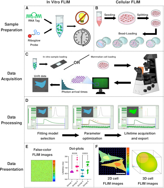
Figure 1: Overview of experimental workflow. A-B) Sample preparation workflow for in vitro (A) and mammalian cell (B) samples. C) FLIM data acquisition workflow. D) FLIM data processing workflow. Collected data are fit using n-exponential reconvolution, the number of fitting parameters are determined for each acquisition, and the final lifetime value is determined and exported. E-F) FLIM data display. In vitro data (E) is presented as false-color FLIM images or lifetime dot-plots, and cellular data (F) is presented as 2D or 3D cell FLIM images. Please click here to view a larger version of this figure.

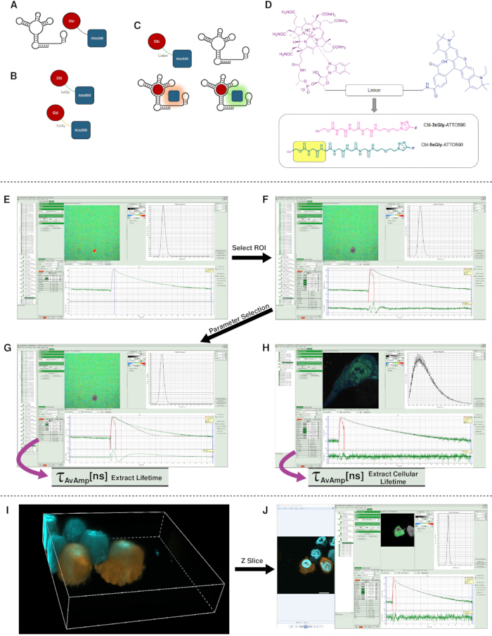
Figure 2: Riboglow platform, linker series, and FLIM fitting workflow. A-B) Cartoon of Riboglow probes and RNA A Tag. C) Illustration of Riboglow probe binding to the RNA aptamer tag (A Tag), which results in increased fluorescence intensity and lifetime upon complex formation. D) Riboglow linker series for this study. Cbl (plum) is covalently coupled to a fluorophore (blue) via a variable chemical linker. 5xGly contains two additional glycine residues, as highlighted in yellow. E-J) FLIM data processing via SymPhoTime 64. E-G) FLIM data is imported into SymPhoTime 64 (E). A clean region of interest (ROI) is selected (F), and decay curves are then fitted using an n-exponential reconvolution model (G). The optimal fit is utilized to obtain the amplitude-weighted average lifetime (τ_AvAmp). H) 2D cellular FLIM analysis of the quenched 3xGly in U-2 OS cells, showing fitting for n = 3. I) 3D volume rendering of HeLa cells labeled with quenched 5xGly and DAPI. J) Z-stack workflow for nucleus versus cytosol FLIM analysis, demonstrating how corresponding confocal z-slices guide a precise ROI placement for compartment-specific lifetime fitting. Please click here to view a larger version of this figure.

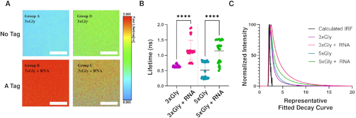
Figure 3: Assessing fluorescence lifetimes of two probe variants in vitro +/- RNA. A) Quantitative visualization of Riboglow probes by fluorescence lifetime imaging microscopy (FLIM) in vitro in the presence or absence of the RNA A Tag. Scale bar = 50 µm. B) Plotted τ _AvAmp values for 3xGly and 5xGly in vitro samples, with and without RNA A Tag. Each point represents one FLIM acquisition. Error bars represent mean and SD. One-way ANOVA with post hoc Tukey HSD reveals significant differences in lifetimes (****p < 0.0001). C) Representative in vitro decay curves for 5xGly and 3xGly probes with and without RNA-A. Please click here to view a larger version of this figure.

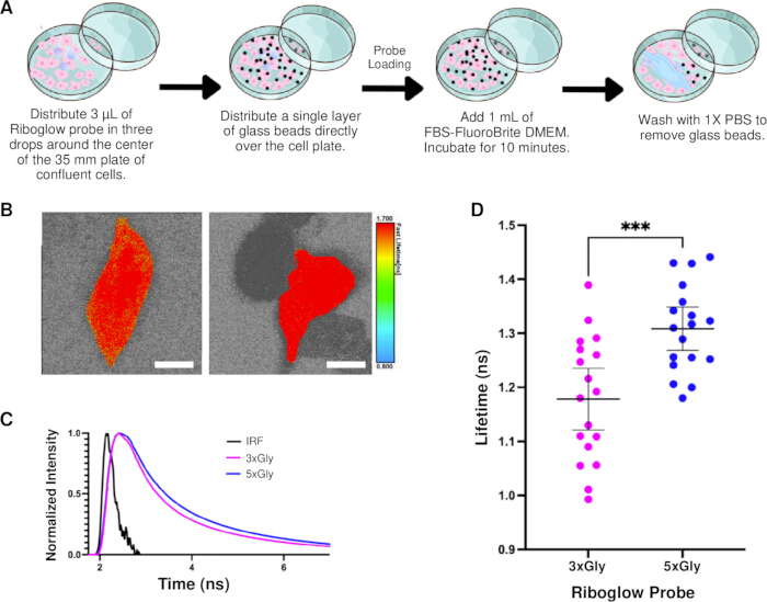
Figure 4: Fluorescence lifetime imaging of HeLa cells with 3xGly (Group E) and 5xGly (Group F) Riboglow probes. (A) Overview of probe loading process. (B) Cellular acquisition images of Group E (left) and F (right). Scale bar = 10 μm. (C) Fitted lifetime decay curves extracted from Groups E and F and plotted with the IRF. (D) Fluorescence lifetime for Group E (n=18 cells) and Group F (n=18 cells) in HeLa cells with mean and 95% CI error bars shown. Unpaired t-test reveals significant difference in lifetimes between cells loaded with 3xGly and 5xGly,*** p < 0.0005. Please click here to view a larger version of this figure.

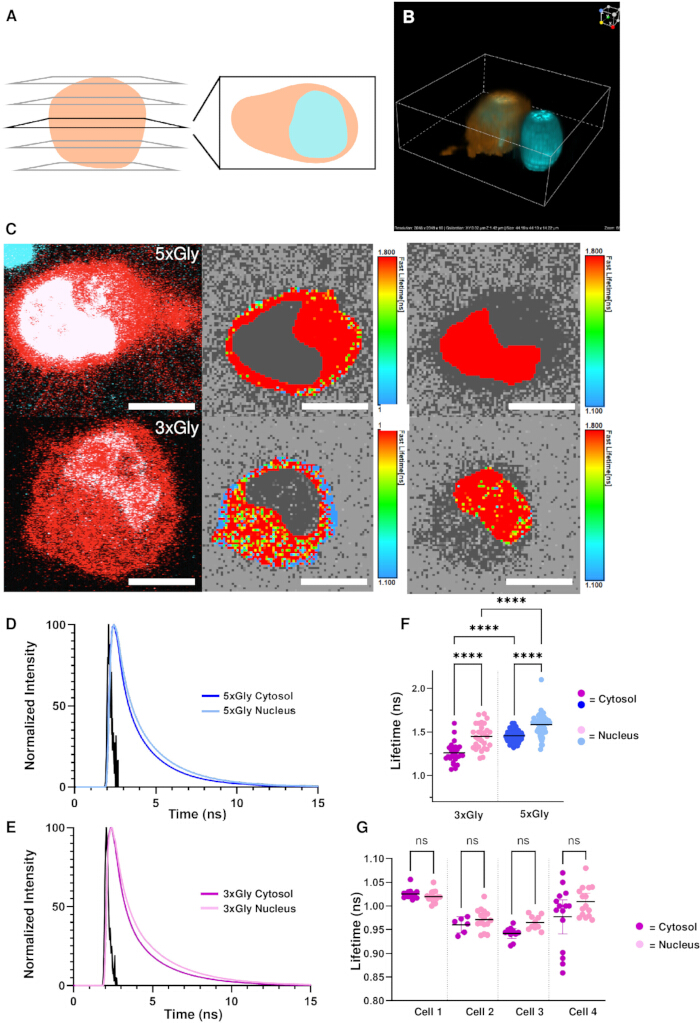
Figure 5: FLIM analysis of subcellular compartments using 3xGly (Group L) and 5xGly (Group M) Riboglow probes. (A) Schematic representation of Z-stack imaging. (B) 3D rendered image of a HeLa cells acquired through confocal Z-stack images. HeLa cells contained a blue nuclear stain (cyan) and were loaded with Riboglow probe (orange). (C) FLIM analysis of bead-loaded HeLa cells. Confocal images (left column) were used as references for ROI selection (middle, right columns). Scale bars = 10 μm. (D-E) Representative fluorescence decay curves extracted from nuclear and cytosolic ROIs of HeLa cells loaded with either (D) 3xGly, or (E) 5xGly. Curves show normalized photon counts versus decay time, and each decay is overlaid with its instrument response function (IRF, black). (F) Dot plot quantifying fluorescence lifetimes from nuclear versus cytosolic ROIs across the two experimental groups. Each point represents a single cellular ROI. One-way ANOVA with post hoc Tukey HSD reveals significant differences in lifetimes between nucleus and cytosol within both groups (****p < 0.0001). (G) Dot plot of fluorescence lifetime Z-stacks of four cells. Each point represents a single ROI taken from one slice of a cellular Z-stack. Multiple ROIs derived from the same cell were treated with caution, as they are not fully independent biological replicates. All ROIs were defined using the confocal image as a reference. Paired t-tests reveal no significant differences in lifetimes between nucleus and cytosol within all cellular Z-stacks (ns p > 0.05). Please click here to view a larger version of this figure.

Discussion

Riboglow-FLIM provides a framework for quantitative RNA imaging by taking advantage of fluorescence lifetime readouts. Successful application of this protocol depends critically on careful control of photon acquisition, decay fitting, and unbiased sampling. Photon counts must be balanced to ensure sufficient statistics for reliable n-exponential reconvolution while avoiding detector saturation, pileup effects, and photobleaching that artificially decrease extracted lifetimes. In practice, insufficient photon numbers most often result in failed fits, especially when using small ROIs in cell imaging such as attempting to resolve small cellular compartments, whereas excessive photon flux compresses decay curves due to binning limitations of TCSPC detection. Selecting appropriate dwell times, frame numbers, and laser power based on experimental goals is therefore essential. Dwell time and frame number together determine the total photon budget by controlling how long each pixel is sampled and how many times the field of view is revisited, respectively, whereas laser power sets the excitation rate and therefore photon yield per dwell period, with direct consequences for signal-to-noise, photobleaching, and pileup. Equally important is avoiding overfitting of decay curves by minimizing model parameters and confirming random residuals, as overparameterization systematically biases lifetime values downward. The choice of lifetime metric is an important analytical consideration, as amplitude weighted (τ_AvAmp) and intensity weighted (τ_AvInt) averages reflect different aspects of multiexponential decay and are not interchangeable. Consistent with prior guidance, τ_AvAmp is used here because it more directly represents the fractional contributions of lifetime components and is better suited for resolving heterogeneous biological environments²³. Accurate determination of the instrument response function (IRF) is required for reliable reconvolution fitting, especially when resolving short lifetime components. A calculated IRF is used to maintain experimental fitting consistency over time yet may introduce systematic error if it deviates from the true instrument response. Periodic measurement of the IRF using a potassium iodide standard should be conducted to verify agreement between measured and calculated IRFs. For cellular experiments, unbiased sampling requires assessment of cell health and probe loading prior to lifetime extraction, as post hoc exclusion based on lifetime outcomes introduces selection bias. Bead-loading introduces additional variability in cell viability, and only cells exhibiting normal morphology and stable fluorescence signal as determined by brightfield or confocal imaging should be included in analysis. Irregular structures such as rounding, blebbing, or dim cells should be excluded²². In our experience, imaging is best completed within approximately 3 h of bead loading to minimize cellular stress, which can alter fluorescence lifetime measurements over time.

Decay curve fitting represents the most common troubleshooting challenge in Riboglow-FLIM experiments. Failed fits can be identified by nonphysical parameters such as negative fit amplitudes (a_n < 0 in FLIM analysis fits), poor overlap between fitted and measured decays, or structured residuals. In many cases, fitting quality can be improved by adjusting the temporal fit boundaries to exclude low-signal or late-time noise while preserving the linear region of the decay on a logarithmic scale. Although this approach slightly reduces lifetime resolution, it minimally affects extracted average lifetimes and allows otherwise usable datasets to be retained. When fitting failures persist despite sufficient photon counts and boundary optimization, exclusion of the acquisition is warranted. For large scale cellular studies, protocol modifications such as preselecting cells by confocal imaging and automating multipoint FLIM acquisitions can substantially increase throughput, though these approaches require stable focus control using the microscope’s perfect focus system to minimize Z-drift during extended imaging sessions. This protocol is demonstrated on a Nikon Ti2 Eclipse AX system with PicoQuant TCSPC hardware, but general acquisition and analysis principles are transferable to other FLIM platforms such as Leica SP8 or Abberior STEDYCON systems provided that equivalent control over photon counting, timing resolution, and detector configuration is maintained. While SymPhoTime 64 is used here for analysis, exported FLIM datasets are compatible with other analysis software packages that support TCSPC-based formats, and users may adapt workflows accordingly.

Several limitations of the method should be considered when designing experiments. First, regions of interest defined during confocal imaging cannot be directly transferred into FLIM analysis software and must instead be redrawn manually for each FLIM dataset, introducing additional analysis time and potential user-dependent variability. Additionally, current FLIM processing workflows require individual analysis of Z-stack slices since volumetric lifetime fitting is not currently supported in SymPhoTime 64, increasing analysis time and fragmenting photon statistics across slices. This fragmentation reduces the effective photon count per measurement and can lower fitting precision in dim regions or small compartments. This limitation becomes impactful in 3D cellular imaging where reduced photon counts per slice and increased system complexity decrease lifetime resolution. Since multiple ROIs are often extracted from the same cell across slices, these measurements are not fully independent, which reduces the effective biological repeats and should be considered in statistical interpretation. Consistent with this constraint, small sample sizes in 3D experiments may obscure biologically meaningful lifetime differences that are apparent in single-cell or 2D analyses due to reduced photon counts in defined ROIs. Additionally, very small or dim subcellular localizations are difficult to fit reliably when spatial resolution or photon density is insufficient, further emphasizing the tradeoff between spatial detail and lifetime precision as sample complexity increases.

Despite these limitations, this protocol addresses an unmet need by providing a detailed and standardized workflow for implementation of Riboglow-FLIM across sample types. While Riboglow has been previously applied using intensity-based measurements, Riboglow-FLIM enables a quantitative and environment-sensitive readout that is largely independent of probe concentration and RNA expression level. Fluorescence lifetime has been reported in prior studies to offer advantages over intensity-based approaches, including reduced sensitivity to probe concentration, photobleaching, and optical path differences. Importantly, no standardized protocol for Riboglow-FLIM acquisition and analysis has previously been published, and the detailed workflow presented here establishes a set of experimental considerations for unbiased data collection, fitting discipline, and interpretation across in vitro, cellular, and 3D systems.

The availability of a validated Riboglow-FLIM protocol expands the experimental toolkit for studying RNA dynamics, localization, and regulation in live cells. This approach is well suited for experiments requiring quantitative comparison across subcellular compartments, time points, or experimental conditions, as well as for multiplexed RNA imaging using orthogonal lifetime signatures. Beyond fundamental RNA biology, this protocol is readily applicable to studies of RNA processing, transport, stress response, and transcriptional regulation in increasingly complex biological models. As FLIM instrumentation and analysis software continue to evolve, the methodology established here provides a foundation for extending lifetime-based RNA imaging into higher dimensional and in vivo systems.

Materials

List of materials used in this article

Name	Company	Catalog Number	Comments
15 mL centrifuge tube	Abdos	P10402	Used for cell culture and to construct the bead loader
Cbl-3xGly-ATTO590	N/A	N/A	Used for detection of RNA in the Riboglow system, synthesis information available here: https://doi.org/10.1021/acschembio.5c00917
Cbl-5xGly-ATTO590	N/A	N/A	Used for detection of RNA in the Riboglow system, synthesis information available here: https://doi.org/10.1021/acschembio.5c00918
Cell detachment media	Gibco	12605-28	Used for cell splitting and transfer
Cell Imaging Dishes	Ibidi	81218-200	Used for live cell imaging
Cell Microscopy DMEM	Gibco	A1896701	Used for live cell imaging
Confocal Microscope System	Nikon	AX	Used for cellular confocal imaging
DMEM	Gibco	1195-092	Used for mammalian cell culture
FBS	Cytiva	SH30910.03	Used to serum supplement DMEM
Fluorescence lifetime imaging (FLIM) analysis software	PicoQuant	SymPhoTime 64, version 2.9, build 5818	Used for FLIM analysis
Glass beads	Millipore Sigma	G4649	Used to bead-load Riboglow probes into live cells
Glass Coverslips	VWR	48368 062	Used for In vitro imaging.
HEPES	Sigma	H3375	Used to make the RNA buffer.
High Yield RNA Synthesis Kit	Thermo Scientific	K0441	RNA transcription kit
Hybrid Photomultiplier Detector	PicoQuant	PMA Hybrid Series	used for times photon detection for fluorescence lifetime measurement.
KCl	Fisher Scientific	BP366	Used to make the RNA buffer.
Live Cell Nuclei Stain	Invitrogen	R37605	Used to stain cellular nuclei during live cell imaging
Mammalian Cell Cryo Tubes	Fisher Scientific	12-567-501	Used for mammalian cell storage
MgCl2	Sigma	M8266	Used to make the RNA buffer.
Microcentrifuge Tubes	Thermo Scientific	90410	Used in general in-vitro and cell culture work
Microscope Base	Nikon	Ti2 Eclipse	Used for in vitro and cellular imaging.
Microscope Objective	Nikon	N Plan Apochromat	Used for in vitro and cellular imaging.
Microscope Operation Software/Image Acquisition and Analysis Software	Nikon	NIS-Elements, version 6.20.02.
Microvolume Spectrophotometer	Thermo Scientific	ND-2000	Used for DNA and RNA concentration and purity determination
Multichannel Event Timer	PicoQuant	MultiHarp 150	Used for TCSPC to extract fluorescence lifetime from in vitro and cellular samples.
NaCl	Fisher Scientific	BP358	Used to make the RNA buffer.
PBS, 1X	Corning	21-040-CV	Used for cell washes and bead removal
Pulsed Diode Laser and Laser Combining Unit	PicoQuant	Sepia PDL 828, PicoQuant LCU	Used for laser excitation of in vitro and cellular samples.
RNA Cleanup Kit	New England Biolabs	T2050L	RNA clean-up kit
RNAse denaturant	Invitrogen	AM9780	Used to prepare an RNAse-free environment
Tissue Culture Dishes	Fisher Scientific	FB012923	Used for general cell culture and upkeep

References

- Bertrand, E., Chartrand, P., Schaefer, M., Shenoy, S. M., Singer, R. H., et al. Localization of ASH1 mRNA Particles in Living Yeast. Molecular Cell. 2 (4), 437-445 (1998).
- Johansson, H. E., Liljas, L., Uhlenbeck, O. C. RNA Recognition by the MS2 Phage Coat Protein. Seminars in Virology. 8 (3), 176-185 (1997).
- Braselmann, E., Rathbun, C., Richards, E. M., Palmer, A. E. Illuminating RNA Biology: Tools for Imaging RNA in Live Mammalian Cells. Cell Chemical Biology. 27 (8), 891-903 (2020).
- Paige, J. S., Wu, K. Y., Jaffrey, S. R. RNA Mimics of Green Fluorescent Protein. Science. 333 (6042), 642-646 (2011).
- Filonov, G. S., Moon, J. D., Svensen, N., Jaffrey, S. R. Broccoli: Rapid Selection of an RNA Mimic of Green Fluorescent Protein by Fluorescence-Based Selection and Directed Evolution. Journal of the American Chemical Society. 136 (46), 16299-16308 (2014).
- Song, W., et al. Imaging RNA polymerase III transcription using a photostable RNA–fluorophore complex. Nature Chemical Biology. 13 (11), 1187-1194 (2017).
- Dolgosheina, E. V., et al. RNA Mango Aptamer-Fluorophore: A Bright, High-Affinity Complex for RNA Labeling and Tracking. ACS Chemical Biology. 9 (10), 2412-2420 (2014).
- Chen, X., et al. Visualizing RNA dynamics in live cells with bright and stable fluorescent RNAs. Nature Biotechnology. 37 (11), 1287-1293 (2019).
- Sunbul, M., et al. Super-resolution RNA imaging using a rhodamine-binding aptamer with fast exchange kinetics. Nature Biotechnology. 39 (6), 686-690 (2021).
- Chen, M., et al. A molecular beacon-based approach for live-cell imaging of RNA transcripts with minimal target engineering at the single-molecule level. Scientific Reports. 7 (1), 1550(2017).
- Raj, A., Van Den Bogaard, P., Rifkin, S. A., Van Oudenaarden, A., Tyagi, S. Imaging individual mRNA molecules using multiple singly labeled probes. Nature Methods. 5 (10), 877-879 (2008).
- Bratu, D. P., Cha, B. -J., Mhlanga, M. M., Kramer, F. R., Tyagi, S. Visualizing the distribution and transport of mRNAs in living cells. Proceedings of the National Academy of Sciences. 100 (23), 13308-13313 (2003).
- Zuo, F., et al. Imaging the dynamics of messenger RNA with a bright and stable green fluorescent RNA. Nature Chemical Biology. 20 (10), 1272-1281 (2024).
- Grün, F., et al. Super-Resolved Protein Imaging Using Bifunctional Light-Up Aptamers. Angewandte Chemie International Edition. 63 (51), e202412810(2024).
- Braselmann, E., et al. A multicolor riboswitch-based platform for imaging of RNA in live mammalian cells. Nature Chemical Biology. 14 (10), 964-971 (2018).
- Sarfraz, N., Moscoso, E., Oertel, T., Lee, H. J., Ranjit, S., et al. Visualizing orthogonal RNAs simultaneously in live mammalian cells by fluorescence lifetime imaging microscopy (FLIM). Nature Communications. 14 (1), 867(2023).
- Sarfraz, N., Shafik, L. K., Stickelman, Z. R., Shankar, U., Moscoso, E., et al. Evaluating Riboglow-FLIM probes for RNA sensing. RSC Chemical Biology. 5 (2), 109-116 (2024).
- Sarfraz, N., et al. Establishing Riboglow-FLIM to visualize noncoding RNAs inside live zebrafish embryos. Biophysical Reports. 3 (4), 100132(2023).
- Datta, R., Heaster, T. M., Sharick, J. T., Gillette, A. A., Skala, M. C. Fluorescence lifetime imaging microscopy: fundamentals and advances in instrumentation, analysis, and applications. Journal of Biomedical Optics. 25 (07), 1(2020).
- Stickelman, Z., Sarfraz, N., Rice, M. K., Lambeck, B. J., Milkovich, S., et al. Expanding the Riboglow-FLIM Toolbox with Different Fluorescence Lifetime-Producing RNA Tags. Biochemistry. 64 (11), 2429-2438 (2025).
- Shafik, L. K., et al. Evaluating Linker Architecture in RNA-Detecting Riboglow Probes and Effects on Fluorescence Turn-On. ACS Chemical Biology. 21 (2), 371-379 (2026).
- Cialek, C. A., Galindo, G., Koch, A. L., Saxton, M. N., Stasevich, T. J. Bead Loading Proteins and Nucleic Acids into Adherent Human Cells. Journal of Visualized Experiments. (172), e62559(2021).
- Sarfraz, N., Braselmann, E. Practical guide to fluorescence lifetime imaging microscopy. Molecular Biology of the Cell. 36 (6), tp1(2025).
Reprints and Permissions