Fast and Illustrative Machine Learning Using the Quantum Fourier Transform

Summary

This machine learning method uses the Quantum Fourier Transform (QFT) to summarize multidimensional data and generate an XY relationship for prediction. Housing price data, including property area, bedrooms, bathrooms, and price, demonstrate normalization, angle encoding, QFT processing, and prediction using the resulting relationship.

Abstract

This protocol describes a Quantum Fourier Transform (QFT)-based computational method for analyzing multidimensional datasets and predicting dependent variables without using neural networks or iterative parameter optimization. Classical numerical data are normalized between zero and one, encoded as rotation angles using quantum RY gates, and processed using QFT on a quantum simulator or quantum hardware. The method generates paired X–Y relationships by applying QFT to feature vectors, both with and without the dependent variable. Housing price data were used to demonstrate the procedure, with property area, number of bedrooms, and number of bathrooms as input variables and house price as the dependent variable. QFT outputs obtained from the input features generated X coordinates, whereas outputs obtained after inclusion of the dependent variable generated Y coordinates. The resulting XY relationships were visualized using scatter plots and trendlines for prediction. The method was additionally applied to heart disease, card-transaction fraud, and loan-approval classification datasets. Quantitative validation using Python on two additional datasets produced reported prediction accuracies of 97.44% and 98.36%, with training times of 324 ms and 3.7 s, respectively. Simulator outputs were also compared with 1,024-shot measurements obtained using superconducting quantum hardware, demonstrating hardware-dependent differences under the tested conditions. These results demonstrate an empirical QFT-based approach for multidimensional data analysis and predictive modeling while identifying theoretical validation, hardware noise, and computational scalability as areas requiring further investigation.

Introduction

Machine learning methods are widely used for prediction, classification, and pattern recognition in applications involving image analysis, audio processing, natural language processing, and generative artificial intelligence (AI). Deep neural networks are commonly used supervised learning models that map multidimensional input vectors, represented as X = (x₁, x₂, x₃, …), to an output variable Y through iterative optimization of weights and biases¹. In neural network architectures, the predicted response is computed using:

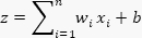
where w_i and b represent learned weights and bias terms, respectively¹. Modern architectures, including transformers, encoder–decoder systems, large language models (LLMs), and generative AI systems, follow related principles but differ in the methods used to combine and process information across layers¹. Although these approaches have demonstrated high predictive capability, their multilevel optimization structure often limits interpretability and contributes to the “black box” nature of AI systems^2,3.

Quantum machine learning has emerged as an alternative computational framework for data analysis and predictive modeling. Variational quantum circuits, also known as parameterized quantum circuits or quantum neural networks, are widely used for supervised learning. Previous work demonstrated the use of variational quantum circuits for retinal condition prediction⁴. However, optimization of variational circuits is affected by barren plateaus, vanishing gradients, and convergence challenges^5,6. These optimization limitations motivate the exploration of alternative quantum computational methods for supervised learning. The present method investigates the use of the Quantum Fourier Transform (QFT) for predictive analysis without iterative parameter optimization.

QFT is a quantum analogue of the discrete Fourier transform and forms the basis of several quantum algorithms, including Shor’s factorization algorithm⁷. Previous studies demonstrated the application of QFT for sound and note detection using both simulators and quantum hardware⁸. Fourier transform methods are robust for signal and pattern analysis because they decompose signals into their constituent frequency components. QFT has also demonstrated computational speedup over classical Fourier transform implementations and has shown structural stability in practical implementations^{9,10,11,12,13}. These properties support the investigation of QFT-based methods for predictive analytics and pattern recognition.

The method described here summarizes multidimensional feature relationships using QFT and visualizes the resulting correlations through XY scatterplots. In supervised learning, labeled datasets establish relationships between input features and output variables. Housing price prediction is an example in which property area, number of bedrooms, and number of bathrooms serve as input variables, while house price serves as the dependent variable. In this protocol, QFT is applied to feature vectors without the dependent variable to generate X coordinates and to feature vectors including the dependent variable to generate Y coordinates. The resulting XY relationship is then used to estimate unknown values that follow similar patterns. The overall workflow of the method is illustrated in Figure 1.

Predictive analytics has applications across multiple sectors, including finance, manufacturing, and healthcare¹⁴. Financial applications include fraud detection, credit scoring, and investment analysis, whereas manufacturing applications include demand forecasting and equipment maintenance. Healthcare applications include patient risk assessment and treatment planning¹⁴. Despite the broad applicability of predictive analytics, limitations such as data quality issues, hidden variables, and dataset bias remain important considerations¹⁵. The method presented here is suitable for datasets containing integer and decimal numerical values.

Quantum circuits used in this study were implemented on an online quantum computing platform that supports graphical circuit design, simulation, and execution on superconducting quantum hardware. A four-qubit QFT circuit consisting of Hadamard and controlled phase-shift gates was initially implemented and later reduced to a three-qubit QFT configuration for selected experiments. The graphical editor and the probability distribution panel for computational basis measurements were used to analyze the output states. Tutorials describing QFT circuit construction can be adapted according to experimental requirements¹⁶. Representative circuit configurations are shown in Figure 2 and Figure 3, and the complete circuit implementation is shown in Figure 4.

The input data were normalized between zero and one using:

The normalized value was multiplied by π/2 and encoded as the rotation angle of R_y gates. For example, the feature vector (0.449, 0.500, 0.400, 0.083) was encoded as π/2 × 0.449, π/2 × 0.500, π/2 × 0.400, and π/2 × 0.083. This procedure corresponds to angle encoding, in which classical data are mapped to qubit rotation angles¹⁷. Previous studies demonstrated that quantum machine learning algorithms frequently encode features into rotational quantum gates and can be mathematically represented as:

where x = [x₁, x₂, …, x_N] represents the feature vector encoded into an N-qubit system^18,19. Details of the angle encoding procedure are illustrated in Figure 5.

Fourier transform methods decompose signals into sine and cosine components at different frequencies, as illustrated in Figure 6. In classical signal processing, the discrete Fourier transform maps an input vector to a frequency-domain representation according to:

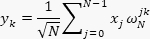
where N represents the number of samples and ω denotes the Fourier basis coefficient¹⁶. QFT extends this operation to quantum basis states and can be efficiently implemented using Hadamard and controlled-phase-shift gates. The Fourier basis representation of a qubit state is given by: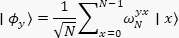
where,

and N represents the number of basis states¹⁶. Representative QFT circuit implementations are shown in Figure 2 and Figure 3.

Quantum computation measurements produce probability distributions over computational basis states. In this study, probability distributions were evaluated using 1,024 measurement shots in a real device. The probability amplitudes of the output state are represented as:

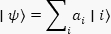
where a_i represents the probability amplitude associated with basis state |i. The probability distribution panel demonstrated that the computational basis state 0000 consistently contained the dominant amplitude contribution. When all R_y gate values were set to π/2 × 1, the probability of state 0000 approached 100%, whereas probabilities of all other states approached zero (Figure 7). When all R_y gate values were set to zero, the probability distribution became uniform across all states, producing equal probabilities of 100/2ⁿ%, where n is the number of qubits. For a four-qubit QFT system, this resulted in probabilities of 6.25% for each computational basis state (Figure 8).

The probability of computational basis state 0000 for angle encoding of qubit q[0] was empirically observed to follow

where,

indicating that the dominant output probability varies as a function of sin(θ), where θ is the encoded rotation angle. These observations suggest that the computational basis state 0000 contains the primary information required for the predictive relationship used in this method. The probability distributions and representative outputs are illustrated in Figure 6, Figure 7, and Figure 8.

The learning procedure involves applying the QFT to the normalized data via angle encoding and obtaining the corresponding probability for the computational basis state 0000. These results are used to generate a set of (x, y) coordinates that establishes a mapping between the input variables and the output variable. The resulting map is used to derive a trendline equation and determine the range of values around the trendline. For prediction, the x value for a previously unseen set of inputs is computed using the same normalization, angle encoding, and QFT procedure used during learning. The corresponding y-value and its prediction range are then determined using the established trendline equation and its associated range.

Protocol

1. Data preparation

1. Select and organize the dataset
   1. Open spreadsheet software and create a new worksheet.
   2. Import the housing dataset into the worksheet²⁰.
   3. Filter the dataset using Data > Filter and select a single property type within one locality and sublocality. Use the following filter settings: LOCALITY = New York County, SUBLOCALITY = New York, and TYPE = House for sale.
   4. Retain only the numerical columns PROPERTYSQFT, BEDS, BATH, and PRICE.
   5. Copy the filtered dataset into a new worksheet labeled “Filtered Data”.
   6. Delete row 9 with outlier.
2. Normalize numerical values
   1. Identify the minimum and maximum values for each numerical column.
   2. Create four additional columns labelled PROPERTYSQFT_norm, BEDS_norm, BATH_norm, and PRICE_norm.
   3. Normalize each numerical value using:
      
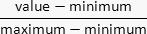
   4. Enter the normalization formula into the first row of each normalized column using absolute references for the minimum and maximum values.
   5. Copy the normalization formula downward to normalize all rows in the worksheet.
   6. Verify that all normalized values are within the range from zero to one.
   7. Save the worksheet.
      NOTE: Use a consistent decimal format across all normalized values to improve readability. Auto-formatting is better for facilitating comparison with the sinusoidal relation in QFT output probabilities.

2. Construction of the QFT circuit

1. Access the quantum circuit platform
   1. Open a web browser.
   2. Navigate to the graphical quantum simulator.
   3. Create a new quantum circuit.
   4. Select a four-qubit quantum register.
2. Build the four-qubit QFT circuit
   1. Place a Hadamard gate on qubit q[3]²¹.
   2. Add controlled phase gates between q[3] (target) and all lower index qubits (control)²².
   3. Assign controlled phase rotation angles according to the standard QFT sequence (Composer Graphical interface accepts ‘pi’ for π): π/2, π/4, and π/8¹⁶.
   4. Repeat the QFT structure for q[2] and q[1] while reducing the number of controlled phase gates appropriately.
   5. Place a Hadamard gate on q[2] and add controlled phase gates to lower qubits.
   6. Place a Hadamard gate on q[1] and add a controlled phase gate to q[0].
   7. Place a Hadamard gate on q[0].
   8. Insert a SWAP gate, as in the QFT circuit, between q[0] and q[3]²³.
   9. Insert a SWAP gate between q[1] and q[2]²³.
   10. Insert a barrier across all qubits to separate the encoding and QFT sections visually.
       NOTE: Use negative phase-rotation values during execution on quantum hardware if hardware errors occur. Representative circuit layouts are illustrated in Figure 2, Figure 3, and Figure 4.

3. Angle encoding and circuit verification

1. Verify QFT probability behavior (in probability panel for composer)
   1. Place an Ry gate on q[0]^17,18,19.
   2. Observe the probability of computational basis state 0000 in the probability panel. Verify that the probability increases from 6.25% to approximately 12.5%.
   3. Place Ry gates on q[1], q[2], and q[3].
   4. Observe the increase in probability of state 0000 after each gate addition. Verify the approximate values of 25%, 50%, and 100%.
   5. Modify the Ry rotation angle of q[0] to
      
   6. Observe the probability reduction of state 0000 to approximately 50%.
   7. Modify the Ry rotation angles of q[1], q[2], and q[3] to zero.
   8. Verify that the probability of state 0000 decreases sequentially to approximately 25%, 12.5%, and 6.25%.
      NOTE: These steps verify the successful implementation of both the QFT circuit and the angle-encoding procedure. Representative probability distributions are shown in Figure 7 and Figure 8.

4. Apply normalized dataset values

1. Generate QFT feature values
   1. Create two new worksheet columns labeled “QFT: Feature” and “QFT: Feature and output”.
   2. Modify the Ry rotation angle of q[0] to
      
      using the normalized PROPERTYSQFT value.
   3. Modify the Ry rotation angle of q[1] to
      
      using the normalized BEDS value.  
   4. Modify the Ry rotation angle of q[2] to
      
      using the normalized BATH value.
   5. Modify the Ry rotation angle of q[3] to zero for the PRICE variable.
      NOTE: Use zero as the PRICE value when generating the “QFT: Feature” coordinate.
   6. Copy the probability value of computational basis state 0000 into the worksheet column labeled “QFT: Feature”. Record the representative value 31.813.
      NOTE: Use the “Show chart data as table” option in the probability panel to copy probability values.
   7. Modify the Ry rotation angle of q[3] to
      
      using the normalized PRICE value.
   8. Copy the probability value of computational basis state 0000 into the worksheet column labeled “QFT: Feature and output”. Record the representative value 35.949.
   9. Repeat steps 4.1.2.–4.1.8. for all rows in the dataset.

5. Plot QFT feature relationships

1. Generate scatter plots using spreadsheet software.
   1. Select the “QFT: Feature” and “QFT: Feature and output” columns in the worksheet.
   2. Generate a scatter plot using Insert > Chart > Scatter Plot.
   3. Assign “QFT: Feature” values to the X-axis.
   4. Assign “QFT: Feature and output” values to the Y-axis.
   5. Add a linear trendline to the scatter plot.
   6. Display the trendline equation on the chart.
      NOTE: Representative XY relationships are illustrated in Figure 1.

6. Estimate actual output values

1. Reverse the QFT relationship
   1. The paired QFT values are related by the equation:
      y = x + x sin(θ)
      where x is the probability when θ = 0 (e.g., First pair (31.813, 35.949) is related, where PRICE = 0.083 as
   2. Calculate θ in radians, using
      
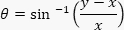
   3. Calculate the normalized price value using
      
   4. Determine the predicted price range from the trendline relationship.
   5. Convert normalized values to original dataset values using
      
   6. Determine the variation range from the trendline and nearest neighbors with maximum deviation.
   7. Verify that the predicted values remain within the calculated range.

7. Validate the prediction method

1. Evaluate prediction consistency
   1. Remove one paired QFT value from the worksheet dataset and regenerate the trendline using the remaining paired values.
   2. Use the updated trendline equation and the remaining X value to estimate the corresponding Y value.
   3. Determine the prediction range by adding the highest deviation of the neighboring values from the trendline. Verify whether the removed QFT value falls within this predicted range.
   4. Repeat steps 7.1.1–7.1.3 for multiple QFT pairs. Record the proportion of removed values that fall within their respective prediction ranges.
      NOTE: A representative validation accuracy of 94.74% was obtained using this procedure.
2. Perform quantitative validation using Python
   1. Clean and filter the first dataset containing 307 observations and four variables by removing missing values, duplicate observations, and outliers to obtain 260 observations. Divide the cleaned dataset into 182 training observations and 78 test observations.
   2. Normalize the four variables using minimum values of 1,000, 1, 1, and 200,000 and maximum values of 10,940, 10, 10, and 39,995,000. Apply the predictive procedure to the training data, evaluate the predictions using the test data, and record the training time and predictive performance.
      NOTE: The observed training time was 324 ms, and the reported accuracy was 97.44%.
   3. Repeat steps 7.2.1–7.2.2 using the second dataset containing 4,801 observations and four variables. After cleaning and filtering, use 3,257 observations, with 2,279 observations for training and 978 observations for testing.
   4. Normalize the second dataset using minimum values of 1,000, 1, 1, and 2,494 and maximum values of 6,000, 10, 10, and 60,000,000. Apply the same predictive and evaluation procedures and record the training time and predictive performance.
      NOTE: The observed training time was 3.7 s, and the reported accuracy was 98.36%.

Results

As outlined in Figure 1, the data were filtered and normalized, and representative house-price data and their corresponding normalized values are presented in Table 1. A four-qubit QFT circuit (Figure 2) or a three-qubit QFT circuit (Figure 3) was constructed according to the number of variables required for the analysis. The complete four-qubit circuit is shown in Figure 4, and the angle-encoding procedure is illustrated in Figure 5. The relationship between the time and frequency domains underlying the Fourier transform is illustrated in Figure 6.

The circuit output was evaluated using the probabilities of the computational basis states. When all normalized input values were set to one, the probability was concentrated in state 0000 (Figure 7). When all normalized input values were set to zero, an approximately uniform probability distribution was obtained across the computational basis states (Figure 8). Table 2 presents the QFT outputs obtained from the normalized values. These QFT values were used to generate the XY scatter plot shown in Figure 9, which represents the relationship between the QFT result obtained from the input features and the QFT result obtained when the output variable was included. The complete spreadsheet is provided as the Supplementary File “NY-House price filtered data with plot,” and the corresponding dataset is provided as “NY-House-Dataset.”

Table 3 presents the original house-price data, corresponding normalized values, and QFT outputs obtained from the input features and from the input features combined with the output variable. These values demonstrate the paired QFT feature and feature-plus-output values used to establish the XY relationship for prediction.  Table 4 presents the filtered heart-disease data, including the normalized values and corresponding QFT outputs. The XY relationships obtained for HeartDisease = 0 and HeartDisease = 1 are shown in Figure 10 and Figure 11, respectively.

Table 5 presents the filtered card-transaction data, the normalized values, the corresponding QFT outputs, and the fraud classifications. The XY relationships obtained for fraud = 0 and fraud = 1 are shown in Figure 12 and Figure 13, respectively. Table 6 presents the filtered loan-approval data, the normalized values, the corresponding QFT outputs, and the loan-status classifications. The XY relationships obtained for Loan_Status = N and Loan_Status = Y are shown in Figure 14 and Figure 15, respectively.

The prediction method was further evaluated using Python on two additional datasets. For the first dataset, 307 observations with four variables were reduced to 260 observations after cleaning and filtering. The cleaned data were divided into 182 training observations and 78 test observations. The analysis resulted in a training time of 324 ms and a reported prediction accuracy of 97.44%. For the second dataset, 4,801 observations with four variables were reduced to 3,257 observations after cleaning and filtering. These data were divided into 2,279 training observations and 978 test observations. The analysis resulted in a training time of 3.7 s and a reported prediction accuracy of 98.36%.

The increase from 260 to 3,257 observations represented an approximately 12.52-fold increase in dataset size, while the measured training time increased from 324 ms to 3.7 s, corresponding to an approximately 11.41-fold increase. Training variational quantum algorithms has previously been described as NP-hard⁶.

Finally, the simulator results were compared with results obtained from quantum hardware using 1,024 shots, as presented in Table 7. When all qubit inputs were set to 1, the simulator produced a probability of 100% for state 0000, whereas the measured probabilities were 32.52% on ibm_kingston, 76.95% on ibm_fez, and 65.33% on ibm_marrakesh. When all inputs were set to 0.5, the simulator probability was 52.53%, compared with hardware probabilities of 59.47%, 53.22%, and 54.10%, respectively. When all inputs were set to 0, the simulator probability was 4.98%, compared with 4.10%, 6.54%, and 9.77%, respectively. Additional measurements obtained by varying individual qubit inputs are also presented in Table 7. These results demonstrated differences between the simulator and quantum-hardware outputs under the tested conditions.

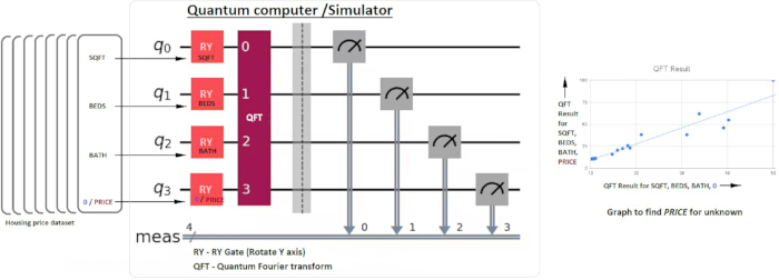
Figure 1: Workflow of the QFT-based prediction method. Data normalization, angle encoding, QFT processing, and generation of the XY relationship are shown. Please click here to view a larger version of this figure.

Figure 2: Four-qubit QFT circuit. QFT circuit configuration for four input variables. Please click here to view a larger version of this figure.

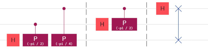
Figure 3: Three-qubit QFT circuit. QFT circuit configuration for three input variables. Please click here to view a larger version of this figure.

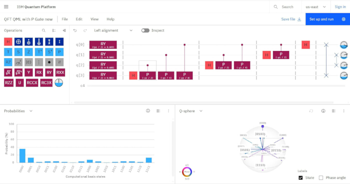
Figure 4: Complete four-qubit QFT circuit. Angle-encoded inputs, QFT operations, and measurements are shown. Please click here to view a larger version of this figure.

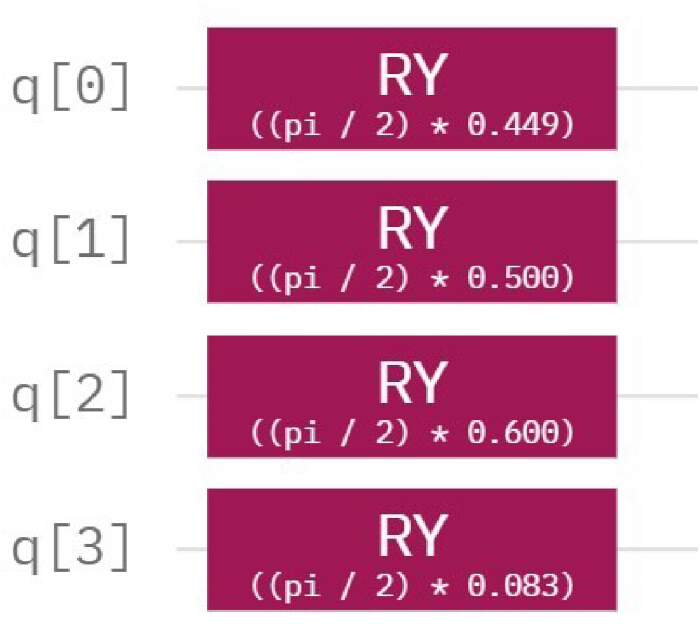
Figure 5: Angle encoding of normalized input values. RY rotations used to encode the normalized values are shown. Please click here to view a larger version of this figure.

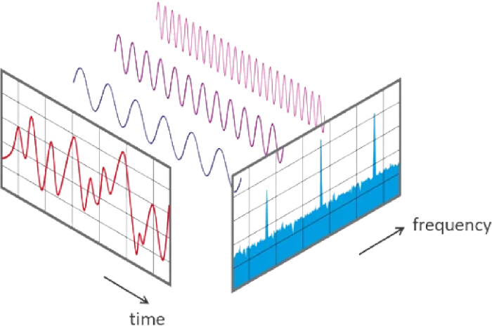
Figure 6: Illustration of the Fourier transform. The transformation from the time domain to the frequency domain is shown. Please click here to view a larger version of this figure.

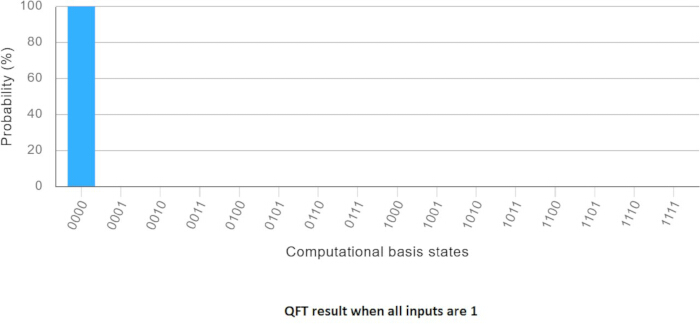
Figure 7: QFT output for normalized input values of 1. Probability distribution across the computational basis states. Please click here to view a larger version of this figure.

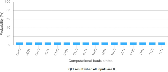
Figure 8: QFT output for normalized input values of 0. Probability distribution across the computational basis states. Please click here to view a larger version of this figure.

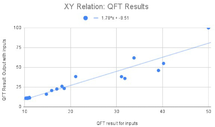
Figure 9: XY relationship of QFT outputs for the house-price dataset. QFT outputs for the input features and for the input features combined with the output variable are shown alongside the fitted trendline. Please click here to view a larger version of this figure.

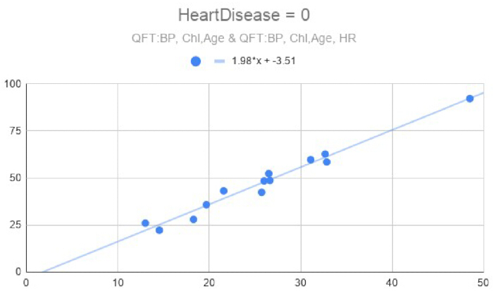
Figure 10: QFT relationship for HeartDisease = 0. XY relationship and fitted trendline for the negative heart-disease class. Please click here to view a larger version of this figure.

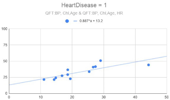
Figure 11: QFT relationship for HeartDisease = 1. XY relationship and fitted trendline for the positive heart-disease class. Please click here to view a larger version of this figure.

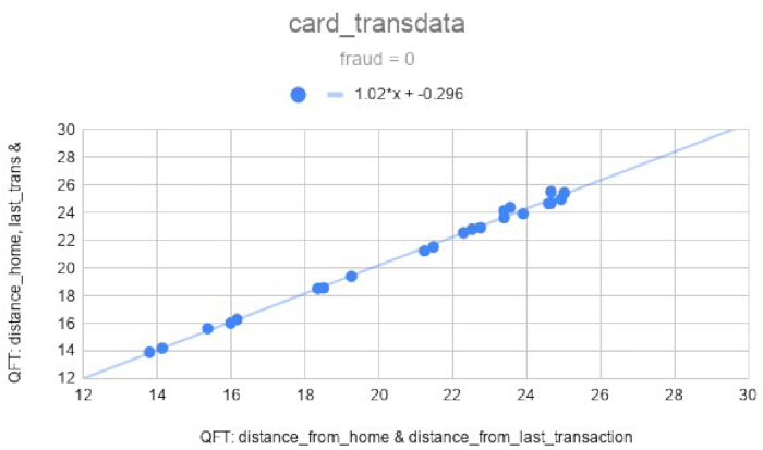
Figure 12: QFT relationship for fraud = 0. XY relationship and fitted trendline for nonfraudulent transactions. Please click here to view a larger version of this figure.

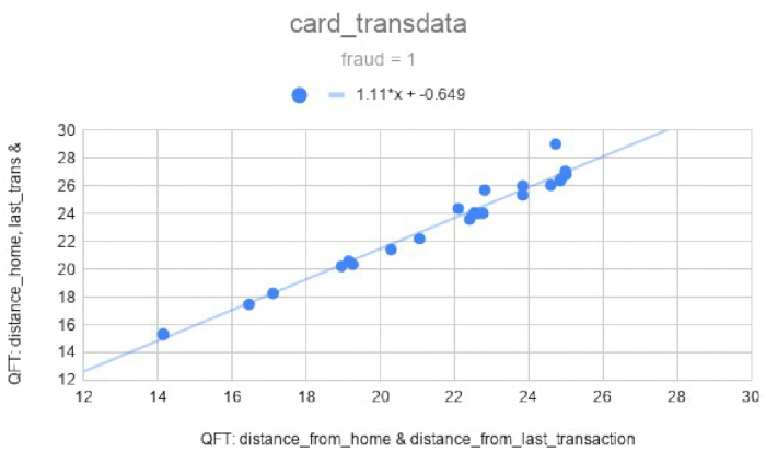
Figure 13: QFT relationship for fraud = 1. XY relationship and fitted trendline for fraudulent transactions. Please click here to view a larger version of this figure.

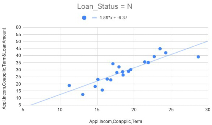
Figure 14: QFT relationship for Loan_Status = N. XY relationship and fitted trendline for non-approved loans. Please click here to view a larger version of this figure.

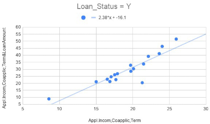
Figure 15: QFT relationship for Loan_Status = Y. XY relationship and fitted trendline for approved loans. Please click here to view a larger version of this figure.

				Normalised
PROPERTYSQFT	BEDS	BATH	PRICE	PROPERTYSQFT	BEDS	BATH	PRICE
2,193.000	3	4	1295000	0.449	0.500	0.600	0.083
1,130.000	2	1	899000	0.178	0.250	0.000	0.046
430.000	3	1	395000	0.000	0.500	0.000	0.000
2,743.000	4	4	1625000	0.589	0.750	0.600	0.113
1,000.000	2	1	879000	0.145	0.250	0.000	0.045
1,198.000	2	2	999999	0.196	0.250	0.200	0.056
2,071.000	3	4	1988800	0.418	0.500	0.600	0.147
3,050.000	2	2	6975000	0.667	0.250	0.200	0.606
2,968.000	4	4	2975000	0.646	0.750	0.600	0.238
2,184.208	1	1	950000	0.447	0.000	0.000	0.051
2,184.208	1	1	680000	0.447	0.000	0.000	0.026
2,184.208	2	2	2150000	0.447	0.250	0.200	0.162
4,108.000	3	3	7188000	0.937	0.500	0.400	0.626
2,046.000	2	2	3498000	0.412	0.250	0.200	0.286
4,357.000	5	6	11250000	1.000	1.000	1.000	1.000
500.000	3	1	635000	0.018	0.500	0.000	0.022
525.000	3	1	485000	0.024	0.500	0.000	0.008
1,750.000	2	2	2695000	0.336	0.250	0.200	0.212
1,471.000	2	2	2499000	0.265	0.250	0.200	0.194

Table 1: House-price data and normalized values. Property, bedroom, bathroom, and price values before and after normalization.

QFT: Feature	QFT: Featr&o/p
31.813	35.949
11.027	11.823
10.669	10.669
39.126	46.035
10.593	11.341
14.740	16.035
31.083	38.197
21.112	38.308
40.227	54.918
10.287	11.110
10.287	10.707
18.618	23.305
33.799	61.931
18.133	26.008
50.000	100.000
10.971	11.350
11.072	11.211
17.009	22.569
15.886	20.653

Table 2: QFT outputs for the house-price dataset. QFT outputs for the input features and input features combined with the output variable.

				Normalised
PROPERTY SQFT	BEDS	BATH	PRICE	PROPERTY SQFT	BEDS	BATH	PRICE	QFT: Feature	QFT: Featr&o/p
2,193.000	3	4	1295000	0.449	0.500	0.600	0.083	31.813	35.949
1,130.000	2	1	899000	0.178	0.250	0.000	0.046	11.027	11.823
430.000	3	1	395000	0.000	0.500	0.000	0.000	10.669	10.669
2,743.000	4	4	1625000	0.589	0.750	0.600	0.113	39.126	46.035
1,000.000	2	1	879000	0.145	0.250	0.000	0.045	10.593	11.341
1,198.000	2	2	999999	0.196	0.250	0.200	0.056	14.740	16.035
2,071.000	3	4	1988800	0.418	0.500	0.600	0.147	31.083	38.197
3,050.000	2	2	6975000	0.667	0.250	0.200	0.606	21.112	38.308
2,968.000	4	4	2975000	0.646	0.750	0.600	0.238	40.227	54.918
2,184.208	1	1	950000	0.447	0.000	0.000	0.051	10.287	11.110
2,184.208	1	1	680000	0.447	0.000	0.000	0.026	10.287	10.707
2,184.208	2	2	2150000	0.447	0.250	0.200	0.162	18.618	23.305
4,108.000	3	3	7188000	0.937	0.500	0.400	0.626	33.799	61.931
2,046.000	2	2	3498000	0.412	0.250	0.200	0.286	18.133	26.008
4,357.000	5	6	11250000	1.000	1.000	1.000	1.000	50.000	100.000
500.000	3	1	635000	0.018	0.500	0.000	0.022	10.971	11.350
525.000	3	1	485000	0.024	0.500	0.000	0.008	11.072	11.211
1,750.000	2	2	2695000	0.336	0.250	0.200	0.212	17.009	22.569
1,471.000	2	2	2499000	0.265	0.250	0.200	0.194	15.886	20.653

Table 3: House-price data and corresponding QFT outputs. Original and normalized values are shown alongside QFT outputs for the input features and for the input features combined with the output variable.

Table 4: QFT results for the heart-disease dataset. Filtered and normalized variables and corresponding QFT outputs for the HeartDisease classes. Please click here to download this file.

Table 5: QFT results for the card-transaction dataset. Filtered and normalized variables and corresponding QFT outputs for the fraud classes. Please click here to download this file.

Table 6: QFT results for the loan-approval dataset. Filtered and normalized variables and corresponding QFT outputs for the loan-status classes. Please click here to download this file.

Input as Ry rotation for all qubits as (pi/2)*	Simulator output for state 0000 in %	Hardware output for 1024 shots on ibm_kingston		Hardware output for 1024 shots on ibm_fez		Hardware output for 1024 shots on ibm_marrakesh
		count	%	count	%	count	%
1	100	333	32.52	788	76.95	669	65.33
0.5	52.53	609	59.47	545	53.22	554	54.10
0	4.98	42	4.10	67	6.54	100	9.77
(q0,q1,q2 = 0) q3 Input=
1	9.86			77	7.52	156	15.23
0.5	8.69			62	6.05	152	14.84
(q0,q1 = 0)q3, q2 Input=
1	21.48			195	19.04	239	23.34
0.5	16.50			160	15.63	176	17.19

Table 7: Comparison of simulator and quantum-hardware outputs. State 0000 probabilities from the simulator and 1,024-shot measurements on ibm_kingston, ibm_fez, and ibm_marrakesh.

Supplementary File 1: Python code. Please click here to download this file.

Discussion

Critical steps in the method include appropriate normalization of the input data, correct construction of the QFT circuit, and verification of the expected circuit outputs. The lowest value of each variable is normalized to 0 and the highest value to 1, with all other values maintained within this range. On a quantum simulator, operation without measurements is preferable because the probability of state 0000 is determined from the circuit output, with the normalized data encoded using R_y(θ), where θ = ^π/₂ × data. This relationship enables mapping of an unknown value from the XY relational scatter plot. Measurements, however, are required when the circuit is executed on real quantum hardware.

Correct implementation of the controlled phase gates is also critical. The controlled phase gate rotation angle is set to ^π/₂ for the nearest qubit, followed by ^π/₄, ^π/₈, and subsequent values according to the circuit structure. A negative sign is added to the P-gate rotation values when required to overcome execution errors on quantum hardware. Circuit operation can be verified using defined input conditions. When R_y(θ) = ^π/₂ × 0, all computational basis states have equal probability. For a four-qubit circuit, this corresponds to 100/2⁴ = 6.25% for each state. When R_y(θ) = ^π/₂ × 1 is applied to all qubits, the probability of state 0000 is 100%, while the probabilities of the other computational basis states are 0%.

The observed relationship between the encoded input and the probability of state 0000 was represented empirically as x + x sin θ, where θ = ^π/₂ × data value, and x represents the probability of state 0000 when θ = ^π/₂ × 0. This empirical relationship was used to describe the observed behavior of the QFT output. Although the Fourier transform theory suggests a relationship involving sin (θ), the specific x + x sin θ relationship used here was derived empirically. Therefore, further theoretical investigation is required to establish its mathematical basis.

An important limitation of the method is its inability to predict values outside the dataset's observed range. The trendline equation provides the estimated trend value, whereas the prediction range depends on the deviations of neighboring data points. Consequently, estimating an output outside the observed data range is difficult and requires further investigation. Interpolation or other suitable approaches may be evaluated for this purpose. Another limitation is that the empirical relationship implemented in the submitted Python code (Supplementary File 1) has not yet been established theoretically. Therefore, the present findings should be interpreted as an empirical demonstration of the method rather than a theoretically established predictive relationship.

The principal features of the method relative to existing or alternative approaches are its simple computational structure and its use of an explicit XY mapping rather than an optimization-based procedure. This representation may facilitate visualization of the relationship between the QFT-transformed input and output values. Potential applications include research areas requiring data analysis, such as bioinformatics, robotics, cheminformatics, advanced engineering, computer networks, banking, and economics. Further investigation across larger, more diverse datasets is required to establish the method's generalizability.

Hardware noise represented an additional limitation. As shown in Table 7, differences were observed between simulator outputs and results obtained from real quantum hardware using 1,024 shots, indicating substantial hardware-dependent error under the tested conditions. The method was also evaluated for dimensional scalability using a simulator in a cloud-based Python notebook environment. The circuit operated satisfactorily with up to 14 qubits but crashed when extended to 15 qubits under the tested computational environment. Thus, the current scalability is constrained by the available simulator and computational resources. Additional studies using larger datasets, repeated hardware executions, and further theoretical and computational analyses are required to characterize hardware variability, computational overhead, dimensional scalability, and the method's broader applicability.

Materials

List of materials used in this article

Name	Company	Catalog Number	Comments
Card_transdata	Kaggle	N/A	Dataset used for fraud-classification analysis
Finance Loan Approval Prediction Data	Kaggle	N/A	Dataset used for loan-approval classification analysis
Google Chrome web browser	Google	N/A	Version 148.0.7778.179 (64-bit); used to access the online quantum computing platform
Google Colab	Google	N/A	Cloud-based Python environment used for code execution and scalability testing
Google Sheets	Google	N/A	Spreadsheet software used for data filtering, normalization, tabulation, and scatter-plot generation
Heart Failure Prediction Dataset	Kaggle	N/A	Dataset used for heart-disease classification analysis
IBM Quantum Composer	IBM	N/A	Graphical quantum circuit platform used to construct, simulate, and execute QFT circuits
ibm_marrakesh	IBM Quantum	N/A	Superconducting quantum computing resource used for hardware execution
NY-House-Dataset	Kaggle	N/A	New York Housing Market dataset; source: Nidula Elgiriyewithana
Python	Python Software Foundation	N/A	Used for automated data cleaning, prediction validation, timing analysis, and scalability testing

References

- IBM. What is a Neural Network? [Internet]. IBM; 2021. Available from: https://www.ibm.com/think/topics/neural-networks
- Westenberger J, Schuler K, Schlegel D. Failure of AI projects: understanding the critical factors. Procedia Computer Science. 2022;196:69-76.
- Rudin C. Stop explaining black box machine learning models for high stakes decisions and use interpretable models instead. Nature Machine Intelligence. 2019;1:206-215.
- Naick MR, Rasheed MA, Jayakumar V, Balaji JJ, Lakshminarayanan V. Quantum machine learning prediction model for retinal conditions: performance analysis. In: Applications of Machine Learning 2022. Proceedings of SPIE. 2022;12227:218-226. Available from: https://www.spiedigitallibrary.org/conference-proceedings-of-spie/12227/122270V/Quantum-machine-learning-prediction-model-for-retinal-conditions--performance/10.1117/12.2633672.full. doi:10.1117/12.2633672.
- Larocca M et al. Barren plateaus in variational quantum computing. Nature Reviews Physics. 2025;7(4):174-189.
- Bittel L, Kliesch M. Training variational quantum algorithms is NP-hard. Physical Review Letters. 2021;127(12):120502.
- Shor PW. Polynomial-time algorithms for prime factorization and discrete logarithms on a quantum computer. SIAM Review. 1999;41(2):303-332.
- Kashani S, Alqasemi M, Hammond J. A quantum Fourier transform (QFT) based note detection algorithm [Internet]. arXiv; 2022. Available from: https://arxiv.org/abs/2204.11775.
- Chen J, Stoudenmire EM, White SR. Quantum Fourier transform has small entanglement. PRX Quantum. 2023;4(4):040318.
- Jayasinghe U, Fernando T, Fernando A. A comparative study of quantum Haar wavelet and quantum Fourier transforms for quantum image transmission. Information. 2025;16(11):962.
- Nam YS, Blümel R. Structural stability of the quantum Fourier transform. Quantum Information Processing. 2015;14(4):1179-1192.
- Biahdillah A. An overview of the quantum Fourier transform and its application in machine learning [Master's thesis]. Aalto University School of Science; Finland; 2024. Available from: https://urn.fi/URN:NBN:fi:aalto-202403172747.
- Dixit V, Jian S. Quantum Fourier transform to estimate drive cycles. Scientific Reports. 2022;12(1):654.
- Desai MS, Deshpande PS. A review of predictive analytics: techniques, advantages, related works and applications. Journal of Advanced Artificial Intelligence. 2024;1(3):1-6.
- Robbin I. Pitfalls of predictive modeling [Internet]. Casualty Actuarial Society E-Forum. 2016. Available from: https://forum.casact.org/article/165812-pitfalls-of-predictive-modeling.
- IBM Quantum Learning. Quantum Fourier transform [Internet]. IBM Quantum Learning; 2026. Available from: https://quantum.cloud.ibm.com/learning/en/modules/computer-science/qft
- IBM Quantum Learning. Data encoding [Internet]. IBM Quantum Learning; 2025. Available from: https://quantum.cloud.ibm.com/learning/en/courses/quantum-machine-learning/data-encoding
- Schuld M, Sweke R, Meyer JJ. Effect of data encoding on the expressive power of variational quantum-machine-learning models. Physical Review A. 2021;103(3):032430.
- Ranga D et al. Quantum machine learning: exploring the role of data encoding techniques, challenges, and future directions. Mathematics. 2024;12(21):3318.
- NTi Audio Solutions for Audio & Acoustics. Fast Fourier Transformation FFT [Internet]. NTi Audio Solutions for Audio & Acoustics; 2026. Available from: https://www.nti-audio.com/en/support/know-how/fast-fourier-transformation-fft
- PennyLane. What is a Hadamard gate? [Internet]. PennyLane; 2024. Available from: https://pennylane.ai/qml/glossary/what-is-a-hadamard-gate
- IBM Quantum Documentation. PhaseGate (latest version) [Internet]. IBM Quantum Documentation; 2017. Available from: https://quantum.cloud.ibm.com/docs/en/api/qiskit/qiskit.circuit.library.PhaseGate
- IBM Quantum Documentation. SwapGate (latest version) [Internet]. IBM Quantum Documentation. Available from: https://quantum.cloud.ibm.com/docs/en/api/qiskit/qiskit.circuit.library.SwapGate
Reprints and Permissions
This article has been published
Video Coming Soon