A Novel Asymmetric Fifteen-Level Inverter for Medium Voltage Applications

Summary

This article presents a new 15-level asymmetric multilevel inverter with ten switches and three DC sources. By optimizing switching angles, an AI-based selective harmonic elimination technique lowers THD and boosts efficiency (>97%). Experiments and simulations validate improved power quality, fewer components, and medium-voltage application compatibility.

Abstract

A reduced-switch asymmetric fifteen-level multilevel inverter (MLI) topology for medium-voltage applications is shown in this article, coupled with a selective harmonic elimination (SHE) control technique aided by artificial intelligence (AI). Ten unidirectional switches and three unequal DC sources are used in the suggested arrangement to limit the total standing voltage (TSV) while producing a stepped output voltage. To find the most effective switching angles for various modulation indices, a hybrid control strategy that combines an artificial neural network (ANN) and the Newton-Raphson (NR) method is employed. A low-voltage experimental prototype is used to test the suggested topology's performance, which is assessed using MATLAB/Simulink simulations. The findings show that, under the evaluated operating conditions, the inverter can produce multi-level output waveforms with low lower-order harmonic content and good conversion efficiency. Over the assessed load range, the measured efficiency ranges from 98.6% to 97.1%, and under nominal conditions, total harmonic distortion (THD) is found to be 5.47%. The suggested topology achieves a lower switch count and competitive TSV and harmonic performance under comparable operating assumptions, according to a comparison analysis with a few multilevel inverter topologies from the literature. Nevertheless, because operational circumstances and control procedures are not completely standardized across research, these comparisons are just informative. While the suggested architecture is meant for scalable extension toward medium-voltage applications, experimental validation is carried out utilizing a low-voltage prototype to confirm switching behavior and control capabilities. The results show that the topology and control technique are feasible, even though the experimental validation is carried out at lower voltage levels. To achieve wider applicability, more validation under higher voltage circumstances and standardized benchmarking frameworks are needed.

Introduction

As a widely recognized renewable energy source, solar energy is attracting a lot of attention in the search for sustainable energy solutions. Solar technology has been widely used due to constant enhancements in efficiency and cost reduction. Solar power is essential for reducing dependency on fossil fuels and slowing down climate change as countries move toward greener energy systems. The cost-effectiveness and environmental advantages of photovoltaic (PV) energy make it unique. The goal of ongoing research and system development is to maximize PV cell energy extraction while guaranteeing smooth grid integration. Multilevel inverters (MLIs) have become an essential technology in recent years because of their capacity to manage large power levels and provide benefits like lower switching losses, better power quality, and less harmonic distortion with improved electromagnetic interference capabilities^1,2,3,4,5.

MLIs use a broad range of DC sources and power electrical circuits made up of several semiconductor switches to create stepped voltage waveforms⁶. As more levels are added, the waveform's quality improves. However, the increasing number of components makes it difficult to achieve good reliability and efficiency, which raises costs⁷. For MLIs to operate well, especially in renewable energy applications, a steady and dependable DC power supply is essential. By controlling voltage levels and lowering fluctuations, DC/DC converters greatly improve voltage quality and system reliability. For example, a robust sliding mode control for a quadratic boost converter, as suggested in⁸, has shown enhanced dynamic response and system stability. In a comparable manner, a comparative analysis of high-gain DC/DC converter topologies in⁹ reveals sophisticated methods for boosting voltage, which qualify them for integration with MLIs in PV applications.

Flying capacitor (FC), cascaded H-bridge (CHB), and diode-clamped or neutral point clamped (NPC) are the three main MLI topologies¹⁰. Several single-phase H-bridge units make up the CHB inverter, which is further divided into symmetric and asymmetric variants according to the DC voltage levels¹¹. Three output levels are produced by conventional CHB inverters: zero, negative, and positive. Each unit's individual output voltage is added up to determine the overall output voltage^12,13. While FC and NPC inverters present difficulties in voltage balancing at higher voltage levels, CHB inverters are favored for medium- and high-voltage applications¹⁴.

A unique structure with fewer switches is suggested in¹⁵, although it has the drawback of requiring several power sources. To address these challenges, the optimal use of semiconductor devices is crucial. An asymmetric inverter topology with bidirectional power switches is presented in¹⁶, which raises the cost of the inverter by increasing the number of IGBTs. Other designs concentrate on raising voltage levels while decreasing the number of power switches^17,18. A full-bridge converter is employed to transform the DC step output created by the systems into an AC step. Because of the voltage-blocking limitations of the full-bridge converter, applications are restricted to high-voltage situations.

Several innovative topologies, such as the three-phase system made up of three single-phase units described in a study¹⁹, are designed to reduce the number of components for single-phase and three-phase systems. Subunit MLIs are used by some topologies to produce multilevel outputs with fewer switches and DC sources²⁰. Bidirectional switches connected in antiparallel are used in some systems to reduce the number of switches and allow current conduction in both directions^21,22,23,24. Blocking voltage across switches is reduced by cascading subunits, creating a modular framework. Nevertheless, an increase in output levels causes a corresponding increase in the number of switches, which is still a disadvantage. Novel MLI configurations that offer various levels while cutting components and blocking voltage are therefore in constant demand, ultimately lowering inverter costs. A new MLI topology called a packed H-bridge has basic units connected on both sides of a whole bridge^25,26. On the other hand, other designs focus on reducing voltage stress on circuit switches by doing away with the H-bridge. However, many of these topologies require many components. To minimize switches, capacitors, and standing voltage while optimizing output voltage steps²⁷, investigates a hybrid cascade multilevel inverter (HCFMLI) design that includes a standard three-leg and H-bridge cells at the bottom section. In a study^28,29, a comparison of cascaded MLI topologies using symmetric and asymmetric configurations is provided.

A study suggests a cascade design for multilevel converters based on sub-multilevel units connected in series, with two ways to calculate the magnitudes of DC sources³⁰. A study describes a sparse 13-level inverter with 14 switches, four capacitors, and two diodes that uses a single DC source to provide a six-fold-boosted output voltage³¹. All possible output voltage levels are produced by the cascade topology suggested in a study³², and comparative analysis shows that it is superior to more modern multilevel converters³³. A single-phase MLI with symmetrical and asymmetrical output voltages is introduced by the topology in another study³⁴. Another research³⁵ offers a single-phase-based multilevel topology that supports an asymmetric DC source configuration, which achieves a 15-level output while reducing space and cost.

Although several fifteen-level inverter topologies have been documented in the literature, different trade-offs in complexity, cost, and harmonic performance are caused by variations in switch count, DC source configuration, and control methodologies. Table 1 summarizes a structural comparison of representative fifteen-level inverter topologies to put the suggested design in context. The comparison focuses on important factors like the number of switches, DC sources, and control strategy. Because operating conditions and evaluation measures vary across research, this comparison is suggestive and based on stated configurations.

This work contribution can be formed into two classifications: (i) a topology contribution, which consists of a fifteen-level inverter based on an asymmetric topology with fewer switches; and (ii) a control contribution, which uses an AI-assisted selective harmonic elimination (SHE) technique to find the best switching angles to remove lower-order harmonics while preserving basic voltage control. The use of an artificial neural network (ANN) to learn the nonlinear relationship between modulation index and optimal switching angles derived from the selective harmonic elimination (SHE) formulation is particularly referred to as "AI-based" in this work. By offering near-optimal initial solutions that are then refined via the Newton-Raphson method, the ANN functions as a data-driven predictor that dramatically reduces computational effort. Compared to solely numerical methods, this hybrid approach allows for quicker convergence and easier practical application.

The key objective is to develop a novel single-phase system design that utilizes an asymmetrical source approach, enabling current conduction with a minimal number of power devices. This article proposes a fifteen-level (15L) inverter for low-voltage applications like solar energy generation, electric automobiles (EVs), and other high-powered specifications. Figure 1 illustrates the connection of rooftop solar panels, Battery, Fuel cells, Super Capacitor, a DC-DC converter, and Electric drive load through the proposed Multilevel Inverter (MLI). Scalable multilevel operation is the main emphasis of the suggested inverter's development. The design concepts are meant to facilitate extension toward medium-voltage applications, subject to suitable device selection, insulation design, and system-level concerns, even if the current work validates the topology using a low-voltage laboratory prototype. The following are the main contributions of this study: 1) A novel asymmetric MLI topology based on CHB, which maintains high output voltage levels while using fewer power semiconductor switches, 2) Optimization of the cost function and total standing voltage (TSV) to increase economy and efficiency and 3) Comparison analysis shows the proposed topology outperforms current systems in terms of efficiency and reduces total harmonic distortion (THD).

Protocol

Topology configuration

Figure 2 displays the recommended architecture, which consists of 10 switches and three voltage sources arranged asymmetrically. The DC sources in the suggested 15-level inverter have a ratio of 1:2:4. This ratio is not arbitrary; it was selected to minimize the number of DC sources while allowing for the creation of a wide range of voltage combinations. The chosen values increase the number of output levels by permitting the production of discrete voltage steps without duplication. All materials used in this study are listed in the Table of Materials.

Switching modes

The switching states for this method are displayed in Figures 3 and 4. Red indicates the conducting path and green the non-conducting path of the matching switches in Figures 3 and 4. Ten switches with three preferred voltage sources are placed to create levels in a natural sequence of magnitude. Table 1 lists the switches that are utilized to produce the necessary voltage levels. In Table 2, 0 denotes nonconductivity, and 1 denotes the conductivity path of the switches. The operating modes of the proposed topology are as follows.

0V_dc: To attain zero voltage in this operating mode, either S₁, S₂, S₃, S₇, and S₉ conducts as depicted Figure 3A.

±1V_dc: S₁, S₅, S₆, S₇, and S₉ conduct in accordance with the modes shown in Figure 3B for acquiring +1V_dc output voltage. To get -1V_dc as output voltage, S₂, S₃, S₄, S₈, and S₁₀ conduct as indicated by the corresponding modes in Figure 4A.

±2V_dc: To obtain +2V_dc as the output voltage, S₃, S₄, S₆, S₇, and S₉ turn on in the manner shown in Figure 3C. S₁, S₂, S₅, S₈, and S₁₀ are conducted in the same way as indicated in Figure 4B mode to achieve an output of -2V_dc.

±3V_dc: To provide +3Vdc output voltage depicted Figure 3D, S₁, S₃, S₆, S₇, and S₉ conducts respectively. As demonstrated in Figure 4C S₂, S₄, S₅, S₈, and S₁₀ conduct in a similar manner to produce -3V_dc output voltage.

±4V_dc: S₁, S₂, S₃, S₇, and S₈ conducts in the manner illustrated in Figure 3E in to operate +4V_dc as the output voltage. S₄, S₅, S₆, S₉, and S₁₀ are conducted in the sequences shown in Figure 4D, to get an output voltage of -4V_dc.

±5V_dc: The switching sequence for generating +5V_dc as output voltage is depicted in Figure 3F. Figure 4E exhibits the conductivity pattern of the switches to provide an output voltage level of -5V_dc.

±6V_dc: The corresponding switching patterns that yield +6V_dc as the output voltage are shown in Figure 3G. Figure 4F shows the switch pattern utilized to deliver an output voltage of -6V_dc.

±7V_dc: S₁, S₃, S₆, S₇, and S₈ conducts as it is shown in Figure 3H to develop output voltage of +7V_dc. S₂, S₄, S₅, S₈, and S₉ conduct as illustrated in Figure 4G to achieve an output voltage of -7V_dc.

Modulation method

In this work, a low-frequency control technique is used for analyzing the efficacy of the proposed inverter. Selective Harmonic Elimination (SHE) takes advantage of a low switching frequency methodology to perform the operation of the MLI. Low-order harmonics are efficiently eliminated via SHE, which additionally minimizes switching losses. However, using this method necessitates resolving several challenging transcendental equations. Figure 4 displays the switching angles taken into consideration for a quarter-wave symmetry. The waveform for an m-level (m is an odd number) output voltage waveform has 2(m-1) switching angles. Figure 5 shows the division of switching angles into four quadrants. Main switching angles are those in the first quadrant, which spans from 0 to π/2. The remaining quadrant angles can be readily determined using the major switching angles.

To reduce the inverter's overall total harmonic distortion (THD), the SHE technique aims to remove lower-order harmonics. Given that the output has 15 levels, the suggested inverter uses SHEPWM to target and eliminate lower-order harmonics like the third, fifth, seventh, ninth, eleventh, and thirteenth. Small filters can be used to successfully suppress higher-order harmonics. The output voltage waveform mathematical expressions are obtained using the Fourier series. The following equations provide these expressions:

(1)

Where a₀= DC component

a_n= Even Harmonic

b_n=Odd Harmonic

In this case

 (2)

 (3)

 (4)

The output waveform quarter-cycle symmetry cancels out the even-order harmonics (a_n = 0) and DC Component(a₀ = 0), leaving just the odd harmonics (b_n). Therefore, the multilevel inverter output equation is expressed as

 (5)

Since it is a 15-level inverter, for one quarter cycle, 7 firing angles are used to determine the peak voltage of each harmonic component. The following equations represent peak harmonic components.

 (6)

 (7)

 (8)

 (9)

 (10)

 (11)

 (12)

It is necessary to adjust the voltage magnitudes of the third, fifth, seventh, ninth, eleventh, and thirteenth order harmonics to zero of the above equations to remove them from the load.

 (13)

The modulation index (M) of the inverter can be computed by

 (14)

The Newton-Raphson (NR) method is used to compute the firing angles, and the main goal of SHE PWM is to reduce harmonic values as much as possible. The NR approach begins the solution of nonlinear equations with an initial estimate, which is a random number between 0 and 90^◦. Iterations with numbers are represented by j and e. The NR approach involves the following actions.

Step 1: To find the firing angles, initial values are set.

 (15)

Step 2: Use the Jacobian matrix for "n" variables in the "k" iterations to calculate the values for the nonlinear equation and dα.

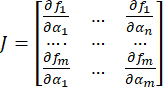  (16)

 (17)

Step 3: If δα is greater than the threshold, repeat step 4. If the threshold is equal to or greater than δα, stop the process.

Step 4: Once Equation (18) has updated the αvalue, move to Step 2.

 (18)

To determine the ideal switching angles, Artificial Neural Networks (ANN) and the Newton-Raphson approach are used. For its training procedure, an ANN needs initial inputs. The internal layers of the artificial neural networks employed in this method are depicted in Figure 6. To provide the ideal switching angles, it consists of two hidden layers (H₁ and H₂) placed between the input and output layers and a single input layer with a value of V_dc. The model is made nonlinear by using a "tanh" activation function, which has a range of -1 to 1′. By assigning a weight to each of their inputs, individual neurons (Y_i) are computed. K is a value between 0 and the number of neurons in the preceding layer. The output values are scaled within the designated range by using the tanh function. The following is a description of this

(19)

It should be mentioned that W_k stands for each neuron's weight, X_k for the kth neuron's output, and Bi for the hidden layer's bias. The error metrics are computed using the mean squared error (MSE) loss. The Back Propagation approach, which uses the Adam optimizer to modify the weights of each layer, is used to lessen error loss.

  (20)

The flowchart in Figure 7 describes the hybrid ANN-NR algorithm's optimization procedure. A hybrid Artificial Neural Network (ANN) and Newton-Raphson (NR) technique is used to guarantee accurate and computationally efficient calculation of optimal switching angles as nonlinear selective harmonic elimination (SHE) equations are solved using the Newton–Raphson method over a modulation index range of 0.6 ≤ M ≤ 1.0 to create the training dataset offline. Valid switching angle sets (α_₁–α₇) that meet harmonic removal requirements for the third, fifth, seventh, ninth, eleventh, and thirteenth harmonics are found and saved for each modulation index,2. One input neuron that represents the modulation index (M), two hidden layers, and seven output neurons that indicate switching angles α_₁ through α₇ make up a feedforward neural network. There are fifteen neurons in the first hidden layer and ten in the second. The output layer has a linear activation function, but the hidden layers employ hyperbolic tangent (tanh) activation functions to add nonlinearity. Both input and output data are standardized to the range [−1, 1] in order to enhance training stability and convergence. Before training, the modulation index and switching angles are appropriately scaled, and during inference, they are rescaled.

The dataset is split 60:20:20 into training, validation, and testing sets. The Adam optimization technique with a learning rate of 0.001 and mean squared error (MSE) as the loss function is used to train the network. To avoid overfitting, training is conducted for up to 1000 epochs with early halting. Training is stopped when the MSE drops below a predetermined threshold or when the validation loss does not improve over 50 consecutive epochs (patience criterion). Initial switching angle estimations for a specific modulation index are provided by the trained ANN during operation. The Newton–Raphson iterative solution then uses these estimations as starting conditions. The NR approach ensures accurate harmonic removal by fine-tuning the ANN outputs to perfectly fulfill the nonlinear SHE equations.

When the residual magnitudes of the intended harmonics (3rd–13th) are less than 0.5%, and the switching angles meet the necessary ordering restriction, a solution is deemed valid:
0 < α₁ < α₂ < α₃ < α₄ < α₅ < α₆ < α₇ < π / 2. Rapid convergence and dependable harmonic suppression over the whole modulation index range are the results of this hybrid ANN–NR strategy, which combines the excellent accuracy of iterative numerical techniques with the quick prediction power of neural networks. Table 2 displays information on several parameters (α₁ to α₇) and measurements (5^th, 7^th, 11^th, and 13^th) for a range of MI values. These numbers appear to reflect measurements or traits associated with the MI values. Figure 8A shows how switching angles vary with respect to the modulation index, and Figure 8B shows how harmonic order varies with respect to the modulation index.

Performance analysis

In this study, we assess the performance of the suggested fifteen-level asymmetric inverter by concentrating on voltage stress distribution, conversion efficiency, power loss characteristics, and device utilization—all of which have a direct impact on practical implementation. The maximum blocking voltages across all switches under various operating conditions are added up to determine the total standing voltage (TSV). We note that voltage stress is not evenly distributed among devices based on the switching states indicated in Table 2. For instance, switches S₁, S₂, S₅, S₉, and S₁₀ encounter blocking voltages of Vdc, 3V_dc, 2V_dc, 4V_dc, and 4V_dc, respectively, at the +6V_dc working level.

For this setup, the peak voltage stress of switching devices connected to the source (V3) is the same, whereas switching devices connected to sources (V1 and V2) have different values. The following equations display the switch's maximum voltage stress.

V_S1 = V_S4 = V₁ = V_dc (21)

V_S3 = V_S5 = V₂ = 2V_dc (22)

V_S2 = V_S6 = V₁ + V₂ = 4V_dc (23)

V_S7 = V_S8 = V_S9 = V_S10 = V₃ = 4V_dc (24)

where V_Sn represents the device maximum voltage stress while it is in the off position. The total standing voltage (TSV) for the proposed design is expressed as (25).

TSV = 2 * V_S1 + 2 * V_S3 + 2 * V_S2 + 4 * V_S7 = 30 V_dc (25)

The asymmetric DC source arrangement and switching sequence directly result in the non-uniform stress profile depicted in Figure 9. The uneven distribution requires careful device rating and selection to prevent overstressing components, even though the overall TSV is lower than with traditional designs. In the framework of the suggested topology, we also evaluate the connection between the number of switches and attainable voltage levels. The current architecture uses 10 switches to accomplish fifteen levels, in contrast to traditional cascaded structures, where level enhancement usually requires proportionate increases in components. According to our investigation, conduction routes are reused across several operating modes to achieve this reduction. Nevertheless, this method restricts simple scalability to higher voltage levels and adds more restrictions to switching logic.

The equation (26) is obtained by computing the cost factor utilizing all the terms that depend on the number of sources (N_s), switch count (N_sw), gate driver circuit count (N_drivers), diode count (N_D), capacitor count (N_C), cost factor (CF), and efficiency. In this case, δ represents the weighting factor. Components are given more weight when δ is less than 1, whereas Total Standing Voltage (TSV) (p.u.) is given more weight when δ is greater than 1. If δ = 1, then the component weights and TSV (p.u.) are equal. For all of the topologies discussed in this study, δ is assumed to be 1.

CF = N_s + N_sw + N_drivers + N_D + N_C + δ*TSV(p.u.) (26)

The efficiency of the inverter is often expressed as equation (27).

 (27)

where power output, power input, and power losses are represented by P_out, P_in, and P_losses, respectively. Switching losses and conduction losses are the three types of power losses in the suggested topology. Switching losses: These losses result from quickly turning devices on and off in a single cycle. The formula is used to express the switching losses brought on by transitions.

 

  (28)

 (29)

The turn-on loss, turn-off loss, and off-state voltage of the ith switch are denoted by P_swlturnon(i), P_swltunoff(i), and V_swoff, respectively. i_on and i_off represent the currents in the switch's on and off states. Equation (30) shows how these losses are added up to determine the overall switching losses (P_sw(Total)).

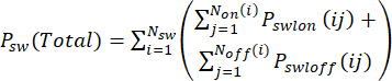 (30)

Conduction losses: A switch's conduction losses are represented as

 (31)

  (32)

where V_don and V_swon represent the on-state voltage drops of the diode and switch, respectively, and P_Dcon and P_swcon represent the conduction losses of the diode and switch. The on-state resistance of the diode and switch is represented by R_Don and R_swon, while the average and RMS currents of the switch are represented by i_Davg, i_swavg, i_Drms, and i_swrms.

For the chosen devices, standard datasheet-based characteristics are used to configure the PLECS semiconductor models. Switching losses (P_on, P_off), conduction parameters (R_Don, V_Don), and thermal resistances are specified using nominal datasheet values and scaled internally by PLECS in accordance with instantaneous operating circumstances when full curve-fitting from manufacturer data is not available.

Using the PLECS simulation platform depicted in Figure 10, we undertake loss analysis to assess power dissipation, considering device-level features for both conduction and switching losses. We find that the distribution of losses changes dramatically depending on the load. Conduction losses predominate under purely resistive loading because certain switches experience constant current flow. On the other hand, phase lag between voltage and current causes switching losses to rise for RL loads, which results in increased energy dissipation during switching transitions. Figures 11A and 11B demonstrate this behavior, with some switches continuously showing larger loss concentrations based on their conduction role.

As shown in Figure 12, the total efficiency of the inverter is calculated by comparing output power to input power throughout a variety of operating conditions (0–2000 W). According to our findings, efficiency drops to 97.1% close to rated circumstances from 98.6% at lower power levels. We explain this tendency by pointing out that when the current magnitude increases, switching and conduction losses contribute more. The observed change suggests that loss mechanisms become more prominent at greater load levels and should be taken into consideration in thermal design, even though the efficiency remains good.

It is crucial to stress that these performance measures are derived under simulation conditions, which presuppose simplified parasitic modeling and idealized switching behavior. In real-world applications, other elements like dead-time insertion, gate driver delays, stray inductances, and temperature-dependent device properties can change efficiency and loss distribution. Consequently, the results do not fully capture all real-world operating impacts, even if they offer a consistent basis for comparison evaluation. TSV, efficiency, and loss distribution are frequently employed as benchmarking criteria in multilevel inverter analysis, and the performance evaluation approach used in this work is in line with accepted procedures in this field. However, we point out that the topology, switching technique, and operating conditions considered in this work are intrinsically dependent on the quantitative results.

The suggested asymmetric fifteen-level inverter and a few multilevel inverter topologies from the literature are contrasted in Table 3. Key structural and performance-related factors, such as switch count, number of DC sources, control technique, and general operating characteristics, are the focus of the comparison. It has been noted that certain current arrangements, such as those in^24,25, use more switches (up to 16) or rely on hybrid or high-frequency modulation techniques, which may result in increased control complexity and switching losses. Although they work under different modulation schemes and design limitations, other reduced-switch topologies, such as²⁷, achieve a lower device count.

Under a low-frequency SHE-based control framework, the suggested architecture produces a fifteen-level output using ten switches and three DC sources. When compared to certain reference designs, the topology exhibits a lower switch count and a moderate total standing voltage (TSV) for this setup and operating state. It should be highlighted, nonetheless, that the provided comparisons are based on data from the literature, and that not all studies use the same operating circumstances, modulation systems, and load assumptions. As a result, it is impossible to prove direct one-to-one performance equivalency. Instead of offering a fully adjusted baseline, the comparison is meant to offer a structural and suggestive assessment. Overall, within the assessed working range, the suggested configuration provides a workable trade-off between component count, control complexity, and harmonic performance.

Results

Simulation results

The fifteen-level operation is simulated using the MATLAB/Simulink interface. The load parameters are 100 Ω and 100 mH, respectively, and the source voltages for fifteen levels are classified as 100 V, 200 V, and 400 V. The suggested inverter operates at 50 Hz, which is its fundamental frequency. The inverter performance under resistive loading conditions is displayed in Figure 13. Figure 14 depicts the inverter operation under various loading scenarios. The inverter operating conditions under various inductive loadings are depicted in Supplementary Figure 1. The resulting waveforms for source voltage fluctuation are shown in Supplementary Figure 2. Supplementary Figure 3 illustrates that the fundamental output of a fifteen-level inverter is 698.9 V, and the associated THD is 5.47%. According to the simulation findings, the suggested inverter functions under all load scenarios.

Experimental results

The hardware prototype created to verify the suggested 15-level inverter topology is shown in Supplementary Figure 4. The precomputed ANN–NR optimized switching angles are used to generate switching pulses in real-time using a TMS320F28379D. To create the necessary asymmetric arrangement, the experimental setup makes use of isolated DC sources with voltages of 10 V, 20 V, and 40 V. Fast recovery diodes (MUR860) and power switches (IRFP460 MOSFETs) with an R-load of 30 Ω and an RL-load of 30 mH are utilized, and a Table of materials used for the experimental test bench is provided.

The output voltage and current waveforms acquired through experimentation under various operating conditions are shown in Supplementary Figures 5–7. The inverter generates a distinct 15-level stepped waveform with a peak output voltage of roughly 70 V and a load current of roughly 1.8 A under resistive loading, with a modulation index of 1.0. The current waveform under RL-load conditions shows the anticipated phase lag relative to the voltage, indicating proper operation under inductive loading. FFT is used for harmonic analysis in order to quantitatively validate performance. The output voltage's measured total harmonic distortion (THD), which is between 5.5 and 6%, closely matches modeling results; small variations can be attributed to non-ideal switching behavior, device parasitics, and measurement uncertainties. The accuracy of the ANN–NR based SHE control technique is confirmed by the effective suppression of lower-order harmonics (3rd–13th).

The inverter functions with fewer effective voltage levels (seen as 13-level behavior) at a lower modulation index of 0.8, which is in line with the theoretical SHE solution space. Despite this, harmonic performance stays within reasonable bounds, proving the control method's resilience over modulation ranges. In terms of waveform shape, harmonic spectrum, and THD values, a comparison of simulation and experimental findings reveals good agreement, with variations staying within allowable bounds (<2%). Practical considerations, including component tolerances, dead-time effects, and switching delays, are the main cause of these variations.
Overall, the experimental findings verify that the AI-assisted SHE control technique achieves efficient harmonic suppression, high-quality output voltage, and dependable operation under both resistive and inductive loading circumstances and establish the viability of the suggested architecture (Table 4).

The suggested fifteen-level asymmetric inverter can produce the desired stepped output voltage under both resistive and resistive–inductive loading circumstances, according to simulation and experimental studies. As anticipated, the number of effective voltage levels decreases with lower modulation indices, and the inverter generates stable multi-level waveforms throughout the assessed modulation index range. With a measured total harmonic distortion (THD) of 5.47% under nominal conditions, harmonic analysis shows that the AI-assisted selective harmonic removal strategy greatly reduces lower-order harmonics. The results of the efficiency evaluation range from 97.1% close to rated operation to 98.6% at lower output power levels. With a few small exceptions due to real-world non-idealities, experimental and simulation results closely match. Together, these findings show that the suggested topology and control approach are feasible under the tested operating conditions.

DATA AVAILABILITY:

Raw data files are uploaded separately as a supplementary zip file.

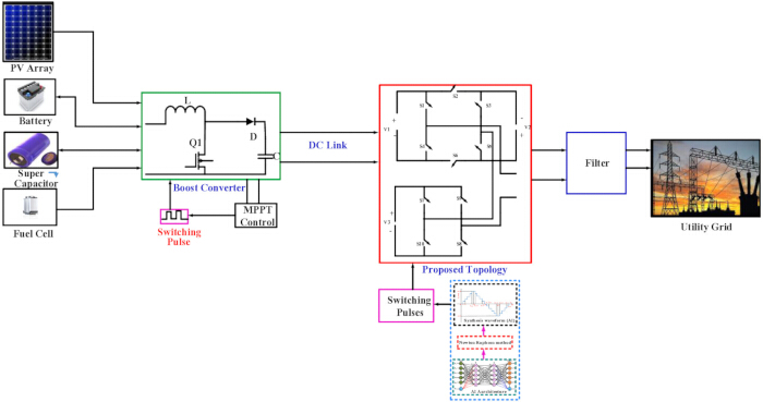
Figure 1: Interconnection of MLI. This figure shows the interconnection of MLI. Please click here to view a larger version of this figure.

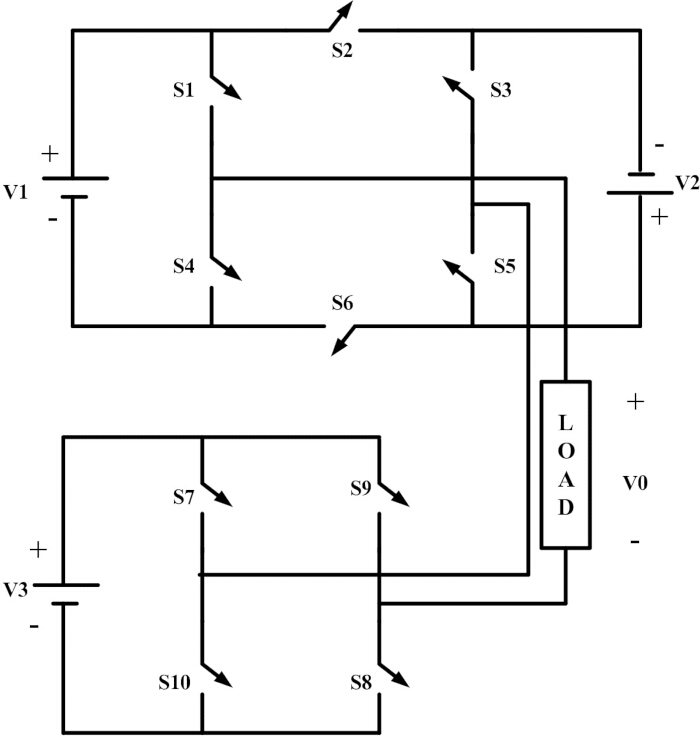
Figure 2: Positive and zero operating states. This figure shows the operating states of the inverter. Please click here to view a larger version of this figure.

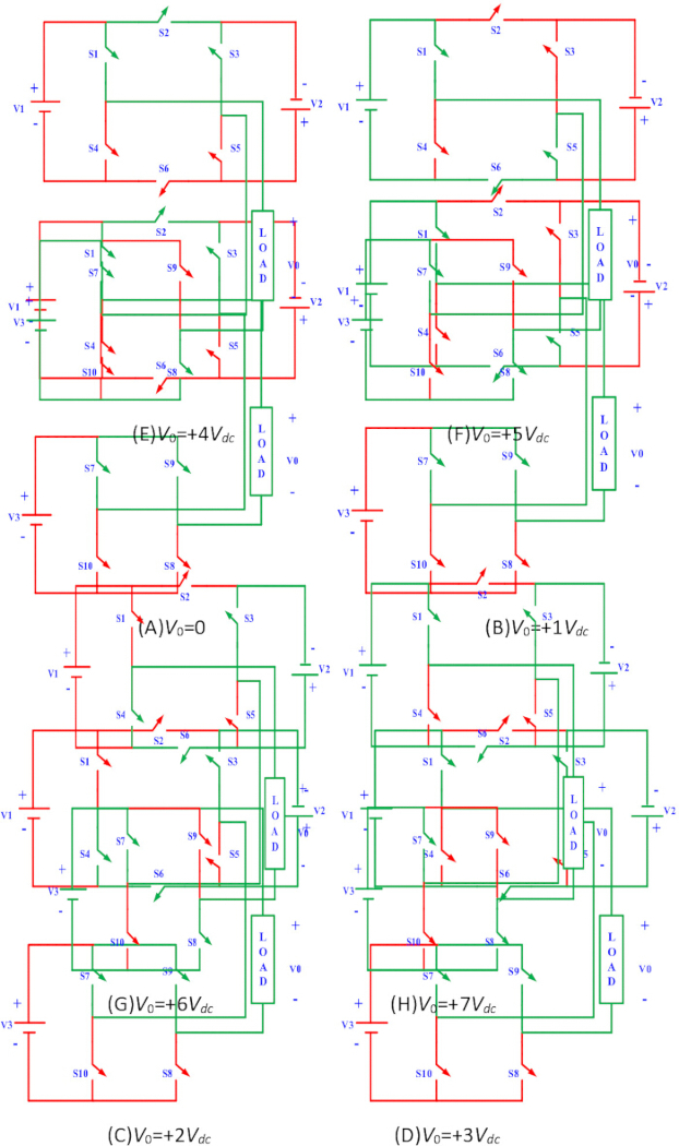
Figure 3: Negative operating modes. This figure shows the negative operating modes of the inverter. Please click here to view a larger version of this figure.

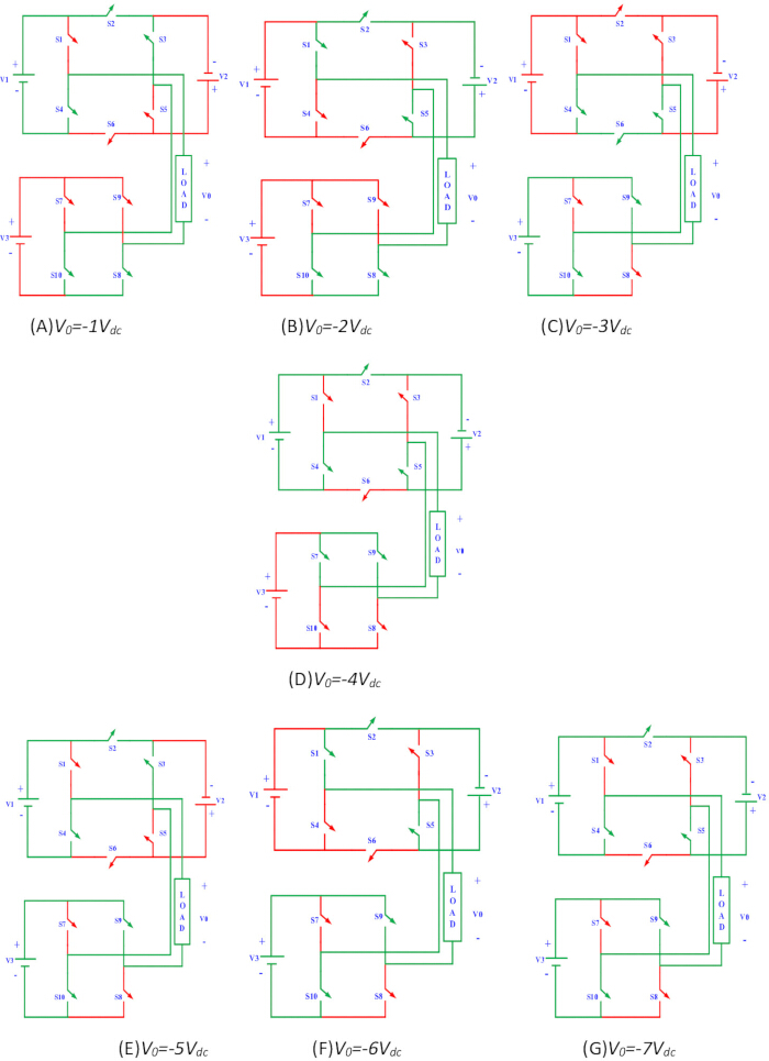
Figure 4: Synthesis waveform. This figure shows the synthesis waveform of the inverter. Please click here to view a larger version of this figure.

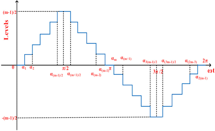
Figure 5: AI architecture. This figure shows an AI architecture. Please click here to view a larger version of this figure.

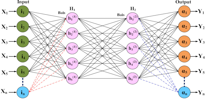
Figure 6: Flow chart. This figure shows the flow of the MLI operation. Please click here to view a larger version of this figure.

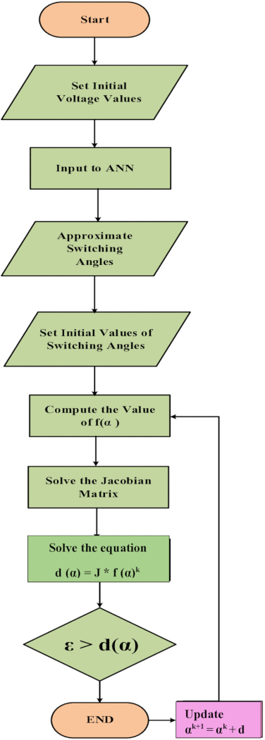
Figure 7: Modulation indexes of MLI. (A) Modulation index vs switching angle. (B) Modulation index Vs Harmonic Component. This figure shows the modulation indexes of MLI. Please click here to view a larger version of this figure.

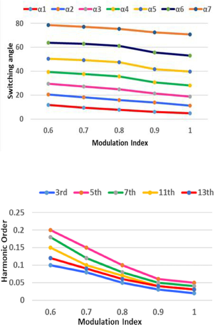
Figure 8: Bar chart representation of voltage stress. This figure shows the voltage stress of MLI. Please click here to view a larger version of this figure.

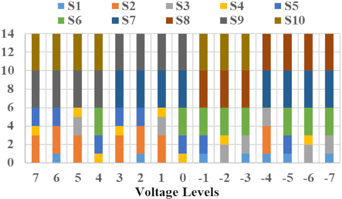
Figure 9: Analysis of switching loss in PLECS environment. This figure shows the switching loss analysis of MLI. Please click here to view a larger version of this figure.

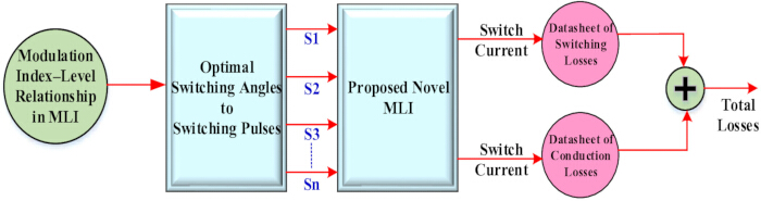
Figure 10: (A) Switching Losses for R-Load. (B) Switching Losses for RL-Load. This figure shows the switching losses for different loads. Please click here to view a larger version of this figure.

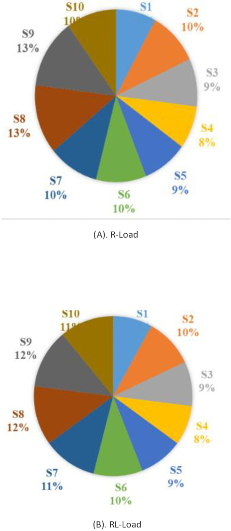
Figure 11: Efficiency curve. This figure shows the efficiency curve of MLI. Please click here to view a larger version of this figure.

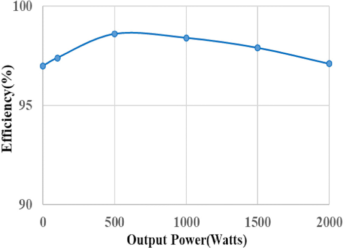
Figure 12: Analysis of waveforms with a resistive Load. This figure shows the R load analysis of MLI. Please click here to view a larger version of this figure.

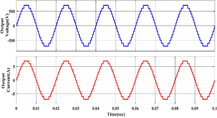
Figure 13: Analysis of waveforms for multiple loading scenarios. This figure shows the multiple loading analysis of MLI. Please click here to view a larger version of this figure.

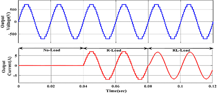
Figure 14: Analysis of waveforms with an RL load. This figure shows the RL load analysis of MLI. Please click here to view a larger version of this figure.

Supplementary Figure 1: Analysis of waveforms for source voltage modulation. This supplementary figure shows the analysis of source voltage modulation. Please click here to download this file.

Supplementary Figure 2: Percentage THD of output voltage. This supplementary figure shows the output voltage %THD. Please click here to download this file.

Supplementary Figure 3: Experimental setup. This supplementary figure shows the experimental test bench.Please click here to download this file.

Supplementary Figure 4: Analysis of waveforms for resistive load (ma = 1). This supplementary figure shows the analysis of waveforms for a resistive load.Please click here to download this file.

Supplementary Figure 5: Analysis of current for RL-load (ma = 1). This supplementary figure shows the analysis of the current wave of RL load.Please click here to download this file.

Supplementary Figure 6: Analysis of waveforms for resistive load (ma = 0.8). This supplementary figure shows the analysis of the current wave of R load with a modulation index of 0.8.Please click here to download this file.

Supplementary Figure 7: Switching pulses. (A–E) This supplementary figure shows the switching pluses. Please click here to download this file.

Switching State	Mode	Output
S1-S3-S6-S7-S8	1	+7Vdc
S3-S4-S6-S7-S8	2	+6Vdc
S1-S5-S6-S7-S8	3	+5Vdc
S1-S2-S3-S7-S8	4	+4Vdc
S1-S3-S6-S7-S9	5	+3Vdc
S3-S4-S6-S7-S9	6	+2Vdc
S1-S5-S6-S7-S9	7	+1Vdc
S1-S2-S3-S7-S9	8	0Vdc
S2-S3-S4-S8-S10	9	-1Vdc
S1-S2-S5-S8-S10	10	-2Vdc
S2-S4-S5-S8-S10	11	-3Vdc
S4-S5-S6-S9-S10	12	-4Vdc
S2-S3-S4-S9-S10	13	-5Vdc
S1-S2-S5-S9-S10	14	-6Vdc
S2-S4-S5-S9-S10	15	-7Vdc

Table 1: Switching states. This table shows the MLI switching states.

Firing angle/Peak Harmonic Component (%)	Modulation Index
	0.6	0.7	0.8	0.9	1
α1	11.8	9.5	7.8	6.2	4.9
α2	20.5	18.2	16	13.8	11.4
α3	29.7	27.4	25	21.5	18.9
α4	39.4	37.6	35.8	30.7	28.1
α5	50.6	49.2	47.6	41.9	39.6
α6	63.8	62.8	61.2	55.6	53.2
α7	78.5	77.1	75.4	72.4	70.8
3rd	0.1	0.08	0.05	0.03	0.02
5th	0.2	0.15	0.1	0.06	0.05
7th	0.18	0.12	0.08	0.05	0.04
11th	0.15	0.1	0.07	0.04	0.03
13th	0.12	0.09	0.06	0.04	0.03

Table 2: Harmonic component analysis for distinct modulation indices. This table shows the Harmonic component analysis for distinct modulation indices.

Topology	NL	NSW	NSW/NL	NDC	TSV (p.u.)	Control	THD (%)
Conventional CHB	15	16	1.07	4	High	PWM/SHE	5–8
[26]	15	14	0.93	3–4	Moderate	HF+LF	4–6
[27]	15	12	0.8	2–3	Moderate	HF	5–7
[25]	15	16	1.07	3–4	Moderate	NLC	4–6
Proposed Topology	15	10	0.67	3	Reduced	AI-SHE (LF)	5.47

Table 3: Comparison with other topologies. This table shows the comparison of the proposed topology with other topologies.

Harmonic	R-Load	RL-Load
Component (%)
3rd	0.22	0.22
5th	0.27	0.27
7th	0.25	0.25
11th	0.23	0.23
13th	0.21	0.21

Table 4: Harmonic component (%) for different Loads. This table shows the harmonic component (%) for different Loads.

Discussion

The reduced-switch asymmetric fifteen-level inverter topology combined with an AI-assisted selective harmonic elimination (SHE) technique is presented in this article. The suggested arrangement is appropriate for medium-voltage applications like solar systems and electric drive interfaces because it strikes a good balance between switch count, total standing voltage (TSV), and harmonic performance. The topology can generate high-quality stepped voltage waveforms with a reported efficiency surpassing 97.1% under nominal operating conditions, consistent with simulation and experimental results. The hybrid ANN–Newton-Raphson (NR) framework, which allows for a faster convergence toward ideal switching angles than traditional iterative-only methods, is a major feature of the suggested method³⁶. This enhances the viability of real-time implementation using DSP platforms and minimizes the computing demand during offline processing. Furthermore, fewer power switches result in simpler gate-driving circuitry and lower conduction losses, both of which are crucial for applications with limited resources.

However, the universality and scalability of the suggested approach are limited by several real-world limitations. The modulation index and initial conditions continue to affect the stability of switching-angle solutions. The NR approach may nevertheless converge to local minima or fail in areas where the nonlinear SHE equations become ill-conditioned, even while the ANN offers reliable beginning estimates³⁷. This makes harmonic performance sensitive throughout the modulation range and requires angle sets to be validated before deployment. Furthermore, the amount of switching angles that are available naturally limits the harmonic removal capabilities. Only specific lower-order harmonics can be addressed with the 15-level arrangement. It is impossible to meet all harmonic elimination requirements at the same time while keeping a valid switching angle ordering at some modulation indices. Total harmonic distortion (THD) may rise outside of ideal operating regions as a result, and residual harmonics continue to exist. This emphasizes the necessity of using hybrid or adaptive modulation techniques when working in a wide range of scenarios.

Practical limitations are also imposed by thermal performance. The asymmetric structure causes uneven voltage stress and power waste among devices, even with fewer switches. According to PLECS simulation results, certain switches undergo greater stress based on conduction paths, which could result in thermal imbalance during prolonged operation. This calls for careful thermal design, especially for high-power applications, which includes choosing the right heat sinking and device rating. The output voltage magnitude, harmonic spectrum, and waveform smoothness show minor variations between simulation and experimental results. Non-idealities such as switching delays, dead-time insertion, oscillations in the DC source, parasitic effects, and finite resolution in DSP-based pulse generation are the cause of the variations. These variations show how crucial it is to take implementation-level limitations into consideration when converting simulation results into hardware, even though they have little impact on general performance.

Finally, scalability remains a challenge. In contrast to traditional cascaded H-bridge (CHB) inverters, which scale modularly, the suggested asymmetric topology necessitates redesigning control equations and switching states for higher voltage levels. The computational load and control complexity would be further increased by expanding the method to 31 or more levels, especially for SHE-based techniques. To overcome these constraints, future research might concentrate on hybrid control methods or modular extensions. In conclusion, under controlled circumstances, the suggested inverter shows great promise in terms of efficiency, fewer components, and harmonic performance. However, a thorough investigation of solution stability, harmonic restrictions, thermal control, and scalability is necessary for its practical implementation. For more widespread adoption in actual power electronic systems, these factors must be addressed.

Materials

List of materials used in this article

Name	Company	Catalog Number	Comments
Current Sensor	Hall-effect sensor	—	Used for current measurement
DC Power Supply (Isolated)	Laboratory Supply	—	10 V, 20 V, 40 V isolated DC sources
Digital Storage Oscilloscope (DSO)	Tektronix	—	Used for waveform observation and measurement
DSP Controller	Texas Instruments	TMS320F28379D	Used for pulse generation and control implementation
Gate Driver Circuit	Custom-built Driver IC	IR2110	Used for MOSFET switching control
Inductive Load	—	—	30 mH inductor
MATLAB/Simulink	MATLAB	Version (2025a)	Used for simulation and analysis
MOSFET	Infineon	IRFP460	500 V, 20 A power switch used in inverter
PCB / Breadboard Setup	Custom	—	Used for hardware implementation
Personal Computer	—	—	Used for simulation and DSP programming
PLECS Software	PLECS	Version (5.0.3.)	Used for thermal and loss analysis
Power Diode	ON Semiconductor	MUR860	600 V, 8 A fast recovery diode
Power Supply Unit	—	—	Auxiliary supply for control and driver circuits
Resistive Load	—	—	30 Ω power resistor
Voltage Probe	Tektronix	—	Used for voltage waveform acquisition