Method Article

Simulation of Condensation Flow and Heat Transfer in Spiral Tube Heat Exchangers for Non-Azeotropic Hydrocarbon Mixtures

37 views

DOI:

10.3791/71595

September 8th, 2026

In This Article

Summary

Here, the article presents a protocol for numerically simulating condensation heat transfer and flow characteristics of non-azeotropic hydrocarbon mixtures in spiral-wound heat exchangers. This method evaluates operational and rolling conditions to predict heat transfer coefficients and pressure drops.

Abstract

As a core component of the natural gas liquefaction process, spiral wound heat exchangers play a crucial role in LNG production. To comprehensively understand the condensation flow and heat transfer characteristics of non-azeotropic hydrocarbon mixtures inside spiral tubes. The high-precision numerical investigation in this study is guided by a well-defined workflow, which involves geometry creation via a professional modeling tool, mesh generation via a dedicated meshing software, numerical computation within a commercial solver (incorporating real-time convergence monitoring), and quantitative post-processing. This integrated approach ensures the high fidelity of the resulting numerical model. The maximum deviations from classical experimental data(Neeraas's experimental data) remain below 15% for the heat transfer coefficient and below 10% for the frictional pressure drop gradient. The simulation results reveal that varying the rolling periods and amplitudes yields similar oscillatory trends in the heat transfer process, exhibiting both enhancement and degradation effects. Specifically, the rolling period alters heat transfer performance by ±20%, whereas the rolling amplitude affects it by ±10%.

Introduction

Natural gas, as a relatively clean fossil fuel, emits significantly less carbon dioxide and other pollutants upon combustion than coal and petroleum. In the global transition toward renewable energy systems, natural gas is often regarded as a "bridge fuel" due to its ability to maintain the stability and reliability of the energy supply1. Through liquefaction, gaseous natural gas is cooled into a cryogenic liquid (LNG), reducing its volume by a factor of approximately 600, which greatly facilitates transportation and storage2. The spiral-wound heat exchanger (SWHE) is a central component in the natural gas liquefaction process. This type of heat exchanger consists of a series of spiral tubes fixed within a cylindrical shell, wound layer by layer in opposite directions around a central mandrel, with spacers separating the layers to ensure sufficient clearance for heat exchange. Due to its spiral configuration, the SWHE provides a large heat transfer surface area within a small footprint3. This compact design makes it highly suitable for integration into large facilities, particularly offshore floating production platforms where space is strictly limited. In the mixed-refrigerant liquefaction processes commonly used in LNG production, non-azeotropic hydrocarbons flow upward inside the tubes, while the shell-side cold fluid flows downward in a countercurrent manner through the gaps within the tube bundle. Under these conditions, the core process on the tube side is the condensation of non-azeotropic hydrocarbons within the spiral tubes, involving complex gas-liquid two-phase flow4,5.

To accurately predict the flow and heat transfer characteristics of condensation inside the tubes, extensive research has been conducted. For single-component alkanes, Fries et al.6 measured the condensation heat transfer characteristics of propane in horizontal tubes, finding that the pressure drop increased as the tube diameter and saturation pressure decreased. They also noted that gravity caused the heat transfer coefficient at the bottom of the tube to be lower than at the top. Zhuang et al.7,8 studied the condensation of methane and ethane in horizontal tubes, showing that the heat transfer coefficient and frictional pressure drop increased with flow rate and vapor quality. A previous study9 analyzed the condensation process of propane in microchannels, confirming that the heat transfer and pressure drop trends were similar to those in conventional channels. For mixed refrigerants, Smit et al.10 investigated the condensation of R22/R142b mixtures in horizontal tubes, finding that at low mass fluxes, increasing the R142b mass fraction significantly reduced the heat transfer coefficient. Berrada et al.11 studied an R134a/R23 mixture and found that the temperature glide had little effect on heat transfer under different component ratios. Neeraas conducted experiments on ethane/propane mixtures in spiral tubes, noting that the mixing effect significantly impacted the calculation of the condensation heat transfer coefficient12. In numerical simulations, Li et al.13 simulated the ethane/propane condensation process, showing that the heat transfer coefficient and frictional pressure drop decreased with increasing saturation pressure. Qiu et al.14 introduced the vapor-liquid entrainment effect when simulating propane condensation in spiral tubes; their results showed that considering this effect reduced the deviation between simulation results and experimental data to less than 25%.

Despite extensive research on various working fluids and channel configurations, a substantial gap persists between the pure or binary fluids typically studied in the literature and the multi-component mixtures utilized in industrial LNG production. Specifically, numerical investigations targeting non-azeotropic hydrocarbon mixtures with three or more components within complex flow channels remain remarkably limited15. Additionally, regarding the unique application of offshore LNG platforms, there is still a lack of a comprehensive understanding of how equipment motion caused by the marine environment alters condensation flow and heat transfer behavior. To address these research gaps, this study combines computational fluid dynamics (CFD) simulations with existing experimental data to develop a detailed three-dimensional, two-phase condensation flow model. Compare and analyze the simulated heat transfer coefficient and frictional pressure drop based on classic experimental data. Based on this model, the paper focuses on simulating the condensation process of representative gas-field compositions in spiral tubes, particularly under rolling conditions, to investigate the underlying mechanisms of complex motion on multi-component condensation heat transfer. This study provides a reliable theoretical basis and engineering guidance for the design and optimization of efficient heat exchangers in offshore natural gas liquefaction processes.

Protocol

Since this work focuses on the local heat transfer and pressure drop characteristics during condensation inside the helical tube, a reduced domain can be employed once the flow is fully developed, enabling an accurate representation of local flow and thermal behavior. For validation against experimental data, a three-section helical tube model is constructed based on the physical model proposed by Neeraas12, with a tube diameter of 14 mm, a helix angle of 10°, and a coil diameter of 2 m. The model consists of three regions: a fully developed section (0.6 m), a test section (0.2 m), and a pressure stabilization section (0.2 m). The fully developed section ensures that the flow is sufficiently developed before entering the region of interest. The test section is used for comparison with experimental data and for detailed analysis of local flow and heat transfer characteristics. The pressure stabilization section is designed to maintain outlet pressure stability and to prevent backflow, thereby avoiding interference with the results obtained in the test section. The specific modeling software is sourced from the Table of Materials.

1. Physical model and mesh

  1. Open modeling software. In the bottom status bar, select Sketch Mode, and click the Z–X plane to enter the sketch environment.
  2. In the top toolbar, select the Circle tool. Draw a circle at the origin with a diameter of 14, then press Enter. Click Return to 3D Mode in the top toolbar. The sketch circle will then be converted into a surface.
  3. Select the generated circular surface. Click the Move tool (shortcut: M) in the top toolbar. A triad manipulator (three-axis handle) will appear on the surface. Drag the yellow sphere at the center of the manipulator to the global origin (0, 0, 0), which will serve as the reference for rotation and translation.
  4. Drag the red arrow along the X-axis, enter 1000 mm, and press Enter. Rotation: Click the rotation ring around the X-axis (blue or green arc), enter 10°, and press Enter.
  5. Click the Pull tool (shortcut: P) in the top toolbar and select the circular surface. In the left panel, choose the Revolve option. Then select the Z-axis of the global coordinate system as the axis of rotation. Enable the Helix option in the left panel. Create Volume 1: In the input box or left panel, enter a height of 138.87 mm and an angle of 45.16°, then press Enter. The first fluid domain is generated.
  6. Create Volume 2: Select the new end face of Volume 1. Repeat the helical pull operation, again using the Z-axis as the rotation axis. Enter a height of 69.44 and an angle of 22.58°.
  7. Create Volume 3: Select the new end face of Volume 2. Create Volume 3 with the same parameters as Volume 2 using the same method.
  8. Click the Workbench tab in the top menu bar. Click the Share button. The software will automatically highlight the two faces that intersect among the three volumes. Click the Complete (checkmark) button on the right.
  9. Click the Groups tab in the left panel. Select the initial circular face of the first volume, then click Create Named Selection and define it as the inlet (in).
  10. Select the final circular face of the third volume, press Ctrl + G to create a group, and define it as the outlet (out).
  11. Select the outer cylindrical surfaces of the three volumes and define them as wall boundaries: wall1, wall2, and wall3.
  12. In the structure tree on the left, hold Ctrl and select the three solids. Press Ctrl + G to create a group and rename it as fluid.
  13. Connect the generated geometry to the Mesh module and double-click to open the Meshing software. In the left tree, click Mesh. In the Details panel at the bottom left, expand Sizing and set the Element Size to 3.
  14. Right-click Mesh in the tree, Insert, Sizing. Select the inlet surface (in) as the geometry and click Apply. Set the Element Size to 0.6.
  15. Right-click Mesh, Insert, Inflation. Geometry: Select all three fluid domains and click Apply. Boundary: Select the outer wall surfaces defined as wall, then click Apply. Change the option to First Layer Thickness. First Layer Height: 0.01mm. Maximum Layers: 15. Growth Rate: 1.25.
  16. Right-click Mesh, Insert, Method. Select the three fluid domains and click Apply. In the Method dropdown menu, choose Sweep. Under this Selection, select Manual Source. Choose the inlet surface (in) as the source face and click Apply.
  17. Right-click Mesh in the tree and select Generate Mesh. In this study, the mesh quality was strictly controlled. The minimum Orthogonal Quality of the generated mesh is above 0.90.

2. Simulation software operation

  1. Open the solving software. Go to the File tab, and under Read, select Mesh. Then go to Scale Mesh and set Mesh Was Created In to mm.
  2. In the Solver settings, select the Pressure-Based solver, choose Absolute for velocity formulation, and enable the Transient option for time.
    NOTE: By superimposing the oscillation equation onto a stationary reference case and implementing it via a user-defined function, the moving coordinate framework can represent the oscillating condition.
  3. Click User-Defined, then select Functions. In the Interpreted UDFs section, load the compiled oscillation file.
    NOTE: The resulting motion is expressed as shown in Equation (1). A static-mesh methodology was adopted and implemented using a moving coordinate framework. The fundamental physics of sloshing relies on the relative motion of the fluid with respect to the container boundary. The sloshing excitation is represented as equivalent dynamic acceleration source terms in the momentum equations, enabling a complete reproduction of the dynamic fluid forces on a stationary mesh.
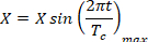
    Harmonic motion equation X=Xsin(2πt/Tc)max, formula, physics, sinusoidal wave analysis.      (1)
    In the equation, Tc represents the swaying period, and X denotes the displacement generated by swaying.
  4. Set the Gravitational acceleration in the Y-direction to −9.81 m/s2. Under Models, enable Energy and turn on the Energy Equation.
  5. Under Models, enable Viscous and select the Reynolds Stress Model (7 equations). In the Reynolds stress model settings, choose Linear Pressure-Strain. For Near-Wall Treatment, select Scalable Wall Functions.
  6. In Phases, set Phase-1 (Primary Phase) as gas and Phase-2 (Secondary Phase) as liquid. Under Global Options, enable Surface Tension Force Modeling, and select the Continuum Surface Force model.
    NOTE: An equivalent pseudo-fluid approach based on temperature- and pressure-dependent thermophysical properties was adopted, which is a widely accepted methodology in CFD studies of multi-component mixtures. Given a fixed initial mixture composition, state-dependent thermophysical properties—including density, dynamic viscosity, thermal conductivity, specific heat capacity, and saturation characteristics—were calculated and generated using the NIST REFPROP database across the entire operating temperature and pressure ranges. In the present study, the mixture maintains a homogeneous macro-composition throughout the simulation. Utilizing NIST-derived variable properties accurately captures the nonlinear thermophysical characteristics of the multi-component fluid while avoiding unnecessary computational overhead.
  7. Taking an ethane–propane mixture as an example, at a vapor quality of 0.56 and a pressure of 3.2 MPa, define the liquid phase properties in Materials as follows:
    1. Density: 393.06 kg/m3
    2. Specific heat capacity (Cp): 3866.4 J/(kg·K)
    3. Thermal conductivity: 0.078798 W/(m·K)
    4. Viscosity: 5.4796 × 10⁻5 Pa·s
    5. Molecular weight: 37.115 kg/kmol
    6. Standard state enthalpy: 0
    7. Reference temperature: 321 K
  8. In Materials, define the gas phase properties as follows:
    1. Density: 67.49 kg/m3
    2. Specific heat capacity (Cp): 3488.7 J/(kg·K)
    3. Thermal conductivity: 0.03035 W/(m·K)
    4. Viscosity: 1.129 × 10⁻5 Pa·s
    5. Molecular weight: 34.756 kg/kmol
    6. Standard state enthalpy: 0
    7. Reference temperature: 321 K
  9. Set the inlet boundary condition as Mass-Flow Inlet(mass flux 300 kg/(m2·s)), the outlet as Pressure Outlet(0 Mpa), and the wall boundary condition as Heat Flux(-10340W/m2).
  10. Under Methods, select the PISO algorithm for solution methods. For Volume Fraction, choose Geo-Reconstruct.
    NOTE: Although the volume-of-fluid (VOF) method is widely accepted for tracking macroscale free-surface topological evolution in sloshing and thermal phase-change processes, inherent limitations persist in interface-capturing precision and in capturing microscale interfacial fluctuations. The VOF formulation fundamentally depends on discrete cell phase volume fractions. The Geo-Reconstruct scheme employed herein significantly alleviates numerical diffusion; nevertheless, resolving subgrid microdroplets, spray formation, or microinterfacial structures remains strictly limited by local grid refinement. For the macro-scale sloshing dynamics, bulk thermal convection, and phase-change mass transfer laws prioritized in this investigation, the current VOF framework with approximately 1.42 million grid elements achieves an optimal balance between topological accuracy and computational cost.
  11. In Monitors, set up monitoring for:
    1. Pressure at the inlet and outlet of the test section.
    2. Temperature at the inlet and outlet.
    3. Wall temperature.
    4. Volume fraction at the inlet and outlet.
      NOTE: The convergence criterion for the energy residual is set to 1 × 10⁻8, while those for the remaining parameters are set to 1 × 10⁻4. Crucial global variables, including the area-weighted average temperature and the total pressure drop across the test section, were dynamically monitored. The computation was continued until these variables showed no further fluctuations, ensuring that the flow field had reached a fully developed and stable state.
  12. Initialize method selection standard initialization, calculate from all zones. After initialization, in the Run Calculation panel, set: Time Step Size: 1 × 10⁻4 s, and Number of Time Steps: 1 × 10⁶.

3. Post-processing and data export configuration

  1. In the Calculation Activities panel, click Autosave (Every Flow Time) to open the Autosave window. In the Autosave settings, set Save Data File Every [s] to 0.01 and specify Flow Time as the save interval type. For Save Associated Case Files Type, select Only if Modified, and then click OK.
  2. Open the Contours window from the Results panel. In the Contours settings, activate the Filled, Node Values, Boundary Values, Global Range, and Auto Range options.
  3. Select Phases as the contour type and Volume Fraction as the variable, then specify phase-1 as the target phase. Finally, click Save/Display to visualize the contour distribution.
    NOTE: The heat transfer coefficient is calculated as the wall heat flux divided by the temperature driving force, obtained from the temperature difference between the inlet and outlet of the test section. Under sloshing conditions, the time-averaged heat transfer coefficient is adopted. The pressure drop is determined by monitoring the difference between the inlet and outlet pressures, and the frictional pressure drop gradient is subsequently calculated as the ratio of this pressure drop to the length of the tube segment.
  4. Import the obtained data into Excel, such as inlet and outlet temperature and pressure values.
  5. Obtain the temperature difference and pressure difference between the inlet and outlet according to the calculation method in section 3.3.

Results

Using the validated numerical model, the actual liquefaction process was simulated to systematically investigate variations in the heat transfer coefficient and frictional pressure drop across different operating parameters, thereby providing a theoretical basis for the design and optimization of heat exchangers. The main conclusions are summarized as follows: for the condensation of a pure fluid, heat transfer is primarily confined to the liquid film adjacent to the tube wall, where the gas-liquid interface temperature equals the core vapor temperature, both of which correspond to the saturation temperature. In contrast, the condensation of a mixture is a non-equilibrium process characterized by simultaneous heat transfer within both the liquid film and the vapor core. Consequently, the gas-liquid interface temperature deviates from the bulk saturation temperature, accompanied by a shift in interfacial concentration from the equilibrium saturated state. During this process, the less-volatile component condenses preferentially, causing the more-volatile component to accumulate at the phase interface. This accumulation elevates the local concentration of the more volatile component, establishing a concentration gradient between the interface and the bulk vapor. This gradient induces a significant mass-transfer resistance that hinders the condensation of the less-volatile component, thereby degrading the condensation heat transfer coefficient.

Volume Fraction Equation:

Partial differential equation for fluid dynamics, involves scalar transport in a mathematical diagram.      (2)

Fluid dynamics equation ∂a/∂t + ∇·(ua) = -S/ρ diagram; conservation of mass principle.      (3)

The gas and liquid phase volume fractions satisfy the following condition:

Static equilibrium formula Σaₗ + aₑ = 1; diagram; educational physics concept.    (4)

Energy equation:

Equation of energy transport in fluid dynamics; includes symbols, differential operators, gradient.    (5)

Phase transition Lee model:

Thermodynamics equation S_al=-r·a_l·ρ_l(T-T_s)/T_s, T≥T_s, related to thermal processes.      (6)

Static equilibrium equation, formula for stress distribution, related to temperature conditions.      (7)

where S(αl) represents the mass transfer rate associated with phase change per unit volume and per unit time; αl represents the liquid phase volume fraction; αg represents the gas phase volume fraction; u⃗ represents the shared velocity of the two-phases m/s; ρ is the mixture density obtained by volume-fraction-weighted averaging kg/m3;µ denotes the dynamic viscosity of the mixture Pa·s; h is the average enthalpy of the gas and liquid phases J/kg; λeff is the effective thermal conductivity between the gas and liquid phases W/(m·K); r is the time relaxation factor 1/s, this article is set to 104; Ts is saturation temperature. The behavior of a mixture of working fluids during condensation differs from that of pure working fluids, primarily due to the volatility of the components.

The mass flux, vapor quality, and saturation pressure have significant effects on the condensation heat transfer coefficient and frictional pressure drop. As the mass flux increases, the flow velocity rises, intensifying the disturbance of the vapor film and thereby enhancing heat transfer within the film, which leads to an overall increase in the heat transfer coefficient. Meanwhile, the shear stress exerted by the vapor phase on the liquid film becomes stronger, resulting in a higher frictional pressure drop. With increasing vapor quality, both the slip ratio between phases and the mixture velocity increase, strengthening the shear interaction between the liquid film and the wall, as well as the interfacial shear between the vapor and liquid phases. This enhances the heat transfer performance. Under these conditions, shear effects become dominant, and the reduction in mixture density further contributes to an increase in the frictional pressure drop. Saturation pressure also plays a critical role in determining the flow and heat transfer characteristics. At low saturation pressures, the vapor density decreases while the flow velocity increases, leading to a thinner liquid film and reduced thermal resistance, thereby enhancing heat transfer. In contrast, at higher saturation pressures, the fluid temperature rises, and the liquid density and viscosity decrease, which weakens the shear interaction between the liquid film and the wall, resulting in a reduction in frictional pressure drop. At a vapor quality of 0.5, as the mass flux increases from 450 to 550 kg/(m2·s), the heat transfer coefficient rises from 5118 to 5637 W/(m2·K), representing a 10% increase. Concurrently, the frictional pressure drop escalates from 2523 to 3442 Pa/m, marking a substantial increase of 36%.

The effects of rolling period and rolling amplitude on the heat transfer process exhibit similar trends, both showing the coexistence of heat transfer enhancement and deterioration. Rolling motion alters the turbulence intensity within the liquid film and consequently affects the turbulent kinetic energy of the film. When the cycle-averaged turbulent kinetic energy increases, turbulence-enhanced transport becomes dominant, leading to improved heat transfer. In contrast, when the cycle-averaged turbulent kinetic energy decreases, the weakening of turbulence suppresses the heat transfer performance. At the same time, rolling motion intensifies fluctuations in the liquid film and alters its thickness. A reduction in liquid film thickness decreases the thermal resistance and therefore enhances heat transfer, whereas an increase in film thickness raises the thermal resistance and weakens the heat transfer performance. These two mechanisms, namely the variation in turbulent kinetic energy and the change in liquid film thickness, interact and jointly determine the overall heat transfer behavior over a rolling cycle. Within the range considered in this study, the influence of rolling period on heat transfer performance is approximately within ±20%, whereas that of rolling amplitude is within ±10%.

Heat exchanger diagram with labeled pressure stabilization and comparison sections; fluid flow process.
Figure 1: Schematic diagram of the simulated physical model. Due to the prohibitive computational cost of simulating full-scale helical tubes, a simplified reduced-domain model is adopted, as shown in Figure 1. For validation against experimental data from Neeraas12, a three-section model is constructed (tube diameter: 14 mm, helix angle: 10°, coil diameter: 2 m). It consists of a fully developed section (0.6 m) to establish flow, a test section (0.2 m) for local data comparison, and a pressure stabilization section (0.2 m) to prevent backflow and maintain outlet pressure stability. It comprises three parts, the first of which is derived from a schematic diagram in a book previously published by Cai1. Please click here to view a larger version of this figure.

Heat transfer vs frictional pressure drop chart; grid number relation; analysis of thermal efficiency.
Figure 2: Results of grid independence. Figure 2 illustrates the grid independence verification results for the heat transfer coefficient and frictional pressure drop as a function of grid number. As shown in the figure, both the heat transfer coefficient and frictional pressure drop decrease significantly as the total cell count increases from 0.60 million to 1.33 million. Beyond 1.33 million cells, the variations in both monitored quantities plateau; further mesh refinement up to 1.85 million cells yields a relative deviation of less than 0.5%, indicating that mesh independence has been achieved. Balancing computational accuracy and resource expenditure, the mesh resolution with approximately 1.42 million cells was adopted for all subsequent simulations. Furthermore, this grid resolution has been verified as suitable for both stationary and swaying conditions. Please click here to view a larger version of this figure.

Bar chart comparing simulation vs experimental data on heat transfer coefficient vs vapor quality.
Figure 3: Verification results of numerical simulation of heat transfer coefficient and Neeraas experimental data. The predicted heat transfer coefficients agree well with the experimental data within the vapor quality range of 0.2–0.8. Specifically, the simulation results are slightly higher than the experimental data at vapor qualities of 0.2–0.4, whereas the experimental values marginally exceed the numerical predictions at vapor qualities of 0.5–0.8. Based on the quantitative evaluation, the maximum deviation is 15%. Please click here to view a larger version of this figure.

Bar chart of frictional pressure drop vs. vapor quality comparing simulation and experimental data.
Figure 4: Verification results of numerical simulation of Frictional pressure drop and Neeraas experimental data. The predicted frictional pressure drop is slightly higher than the experimental results overall, with the maximum deviation not exceeding 10%. Please click here to view a larger version of this figure.

Gas phase volume fraction diagram; flow rates: G=350, 450, 550 kg/m²·s; color scale shown.
Figure 5: Gas phase volume fraction under different mass flux (diameter = 10 mm, vapor quality = 0.5). Figure 5 illustrates the vapor volume-fraction distributions at the outlet cross-section for different mass fluxes at the same vapor quality. As shown in the figure, the minimum vapor volume fraction is 0, indicating that the wall remains completely wetted by the liquid film. At low mass fluxes, the flow pattern is mainly governed by gravity and exhibits a typical stratified-flow structure. As the mass flux increases, the shear stress exerted by the vapor phase on the liquid film becomes progressively stronger and eventually dominates the flow behavior, causing the flow pattern to gradually transition from stratified flow to annular flow. In addition, vapor quality also has an important effect on flow pattern evolution and, together with mass flux, determines the variation in the two-phase flow structure. Please click here to view a larger version of this figure.

Graph of heat transfer vs vapor quality; three curves for different mass fluxes (350-550 kg/m²s).
Figure 6: Heat transfer coefficient under different mass flux. The variation of the heat transfer coefficient with different mass fluxes is shown in Figure 6. At a constant vapor quality, the heat transfer coefficient increases with increasing mass flux. During the condensation process, a vapor film forms along the inner wall of the tube. As the mass flux increases, the flow velocity rises, intensifying the disturbance of the vapor film and enhancing heat transfer within the film, thereby reducing thermal resistance. Consequently, the heat transfer coefficient becomes higher at elevated mass fluxes. Meanwhile, with the increase in mass flux, the Reynolds number corresponding to the liquid film also increases. Overall, the mass flux has a significant effect on the heat transfer coefficient. Please click here to view a larger version of this figure.

Graph of frictional pressure drop vs vapor quality. Lines show G=350, 450, 550 kg/(m²·s) flow rates.
Figure 7: Frictional pressure drop under different mass flux. Figure 7 shows the variation in frictional pressure drop under different mass flux conditions. The results indicate that, at the same vapor quality, the frictional pressure drop increases significantly with increasing mass flux. This is mainly because a higher mass flux leads to a higher flow velocity, which enhances the shear exerted by the vapor phase on the liquid film as well as the wall shear stress, thereby resulting in a larger frictional pressure drop. Overall, mass flux has a pronounced effect on the frictional pressure drop. Please click here to view a larger version of this figure.

Gas phase volume fraction diagram showing color-coded distribution at various values (0.3, 0.5, 0.7, 0.9).
Figure 8: Gas phase volume fraction under different vapor quality (diameter = 10 mm). Figure 8 illustrates the outlet vapor volume-fraction distributions for four vapor qualities. The volume fraction increases sharply at low vapor quality but plateaus near 1 at high vapor quality. Four distinct flow patterns were identified: stratified, semi-annular, annular, and mist flow. At low vapor quality, gravity dominates, yielding a stratified flow with vapor at the top and liquid at the bottom. As vapor quality increases, interfacial shear replaces gravity as the dominant mechanism, driving the flow through semi-annular and annular regimes to mist flow. Please click here to view a larger version of this figure.

Gas phase volume fraction diagram; pressure comparison at 3 MPa and 5 MPa with color scale.
Figure 9: Gas phase volume fraction under different saturation pressures. As the saturation pressure increases, the liquid density decreases, whereas the vapor density increases, leading to a change in the density difference between the two phases and an overall increase in the mixture density. Meanwhile, the gas–liquid slip characteristics are altered, and the interfacial shear between the two phases is weakened, resulting in a reduction in the vapor volume fraction. These variations are more directly reflected in the trends of the heat transfer coefficient and frictional pressure drop. Please click here to view a larger version of this figure.

Bar graph analyzing heat transfer coefficient vs. vapor quality at 3 MPa and 5 MPa pressures.
Figure 10: Heat transfer coefficient under different saturation pressures. Figure 10 shows heat transfer coefficients across different vapor qualities and saturation pressures. At a constant vapor quality, lower saturation pressure yields a higher heat transfer coefficient. Mechanistically, higher pressure increases vapor density, reducing flow velocity and interfacial shear stress. This thickens the liquid film, thereby increasing thermal resistance and degrading heat transfer. Furthermore, the impact of saturation pressure becomes more pronounced at higher vapor qualities, where vapor velocity dominates, and pressure-induced density changes cause larger variations in interfacial shear stress. Please click here to view a larger version of this figure.

Bar graph of frictional pressure drop vs. vapor quality at 3 Mpa and 5 Mpa, illustrating fluid flow dynamics.
Figure 11: Frictional pressure drop under different saturation pressures. Figure 11 shows the variation in frictional pressure drop under different saturation pressures. The results indicate that at the same vapor quality, the frictional pressure drop decreases as saturation pressure increases. Combined with the velocity distribution, subcooling temperature field, and vapor volume fraction distribution at different saturation pressures, these results indicate that higher saturation pressure corresponds to higher fluid temperature, accompanied by decreases in both liquid density and viscosity. As a result, the shear interaction between the liquid film and the wall is weakened, leading to a reduction in frictional pressure drop. Please click here to view a larger version of this figure.

Gas phase volume fraction; simulation results; different time ratios; color mapping; fluid dynamics.
Figure 12: Gas phase volume fraction under different rolling periods (vapor quality = 0.5, mass flux = 550 kg/(m2·s, A = 3 m). At a fixed rolling amplitude, a shorter rolling period leads to a stronger additional inertial effect induced by the oscillatory motion, resulting in more intense velocity fluctuations in the flow field. These fluctuations also exhibit a pronounced periodic behavior, with alternating phases of flow acceleration and deceleration. Meanwhile, rolling motion modifies the spatial distribution of the liquid film and alters the flow pattern, thereby affecting heat transfer. As the average liquid film thickness increases, the film's thermal resistance rises, weakening heat transfer performance. In contrast, as the average liquid film thickness decreases, the film's thermal resistance decreases, thereby enhancing heat transfer. The classification of flow regimes is based on the flow pattern transition criteria proposed in Reference4. Please click here to view a larger version of this figure.

Heat transfer coefficient graph, stationary vs rolling condition; heat exchange analysis results.
Figure 13: Heat transfer coefficient under different rolling periods. Figure 13 compares time-averaged heat transfer coefficients (HTCs) under rolling motion against the stationary baseline. Rolling alters the HTC within ±20%, exhibiting both enhancement and deterioration. At low HTCs (lower vapor quality), rolling enhances heat transfer—more so with shorter rolling periods—by intensifying turbulence in the liquid film and interfacial fluctuations. Conversely, at high HTCs (higher vapor quality), rolling impairs heat transfer by compressing the vapor core and increasing the liquid film thickness (via mean thickening and centrifugal effects in annular flow), thereby elevating thermal resistance. Consequently, a suitable design margin is recommended for offshore applications. Each data point in the figure corresponds to an independent and deterministic numerical simulation case. The CFD solution of the governing equations does not incorporate measurement noise, omitting the statistical variance inherent in repeated experimental trials; therefore, error bars based on statistical distributions are neither applicable nor necessary. Please click here to view a larger version of this figure.

Heat transfer coefficient graph; comparison at rolling periods; includes 10% variance indicators.
Figure 14: Heat transfer coefficient under different rolling amplitudes. Figure 14 compares time-averaged heat transfer coefficients (HTCs) under different rolling amplitudes against the stationary baseline. Rolling amplitude alters the HTC within ±10%, exhibiting both enhancement and deterioration. At low HTCs (lower vapor quality), rolling enhances heat transfer—more prominently at larger amplitudes—by intensifying liquid film turbulence and interfacial fluctuations. Conversely, at high HTCs (higher vapor quality), rolling impairs heat transfer by compressing the vapor core and thickening the liquid film (via mean thickening and centrifugal effects in annular flow), thereby increasing thermal resistance. Consequently, an appropriate design margin is recommended for offshore applications. Please click here to view a larger version of this figure.

Mass fluxVaporPressurePipe diameter (mm)Wrapping angle Winding diameter (m)rolling period (s)rolling amplitude (m)
kg/(m2·s)qualityMPa°
350–5500.1–0.93–510422–52–3

Table 1: Simulated working conditions. Table 1 summarizes the simulation conditions for the light hydrocarbon mixture in the liquefaction section of an actual industrial process15. The working fluid consists of methane, propane, isopentane, ethylene, and nitrogen, with a molar ratio of 55.314:1.407:0.04:23.709:19.53. NIST REFPROP-derived properties were used to accurately capture the homogeneous mixture's non-linear behavior across all operating conditions while minimizing computational cost.

Discussion

Crucial for safeguarding simulation reliability, the three-section configuration establishes fully developed flow conditions upstream of the test section and suppresses backflow at the outlet, thereby optimizing the accuracy of predicted outcomes. This viewpoint has also been reflected in previous studies on horizontal pipes1. During the grid generation process in this study, the first-layer mesh height, the number of boundary layers, and the minimum orthogonal quality requirement are equally critical, as they directly affect the accuracy of the simulation results. Mass flux, vapor quality, and saturation pressure significantly affect condensation heat transfer and pressure drop. Increasing mass flux enhances vapor velocity and interfacial shear, thereby increasing both the heat transfer coefficient and frictional pressure drop. Increasing vapor quality also strengthens interfacial shear and promotes the transition from stratified flow toward annular and mist flow. In contrast, increasing saturation pressure reduces both the heat transfer coefficient and frictional pressure drop. These trends are generally consistent with previous experimental and numerical studies of hydrocarbon condensation6,7,8,9,13. For non-azeotropic mixtures, additional mass-transfer resistance caused by component redistribution near the vapor–liquid interface should also be considered10,11,12.

An important finding is that rolling motion can either enhance or deteriorate condensation heat transfer. Within the investigated range, the rolling period changes the heat transfer performance by approximately ±20%, while the rolling amplitude produces variations of approximately ±10%. This behavior mainly results from the combined effects of liquid-film turbulence and film-thickness variation. Increased turbulence or a thinner liquid film enhances heat transfer, whereas reduced turbulence or film thickening leads to deterioration. Therefore, the overall heat transfer response depends on the competition between these two mechanisms. Several numerical issues should be considered when applying this method. Since the predicted heat transfer and pressure drop are sensitive to liquid-film thickness and interfacial behavior, sufficient near-wall mesh resolution and an appropriate time step are necessary. In addition, convergence should not be evaluated only from residuals. Key physical quantities, including temperature, pressure, vapor volume fraction, and pressure drop, should also be monitored to distinguish numerical oscillations from actual rolling-induced fluctuations.

However, only a limited number of rolling conditions were considered in this study, and broader parametric investigations are still required to obtain a more comprehensive understanding of the influence of dynamic operating conditions on condensation performance. In practical offshore LNG applications, heat exchangers may experience complex six-degree-of-freedom motions caused by vessel movement, including combined rolling, pitching, and yawing motions. These dynamic effects can continuously modify the gravitational field, secondary flow structures, and liquid film distribution inside the helical tube, thereby affecting local heat transfer and pressure drop characteristics. Therefore, future studies should investigate the coupled effects of different rolling amplitudes, frequencies, and motion directions to establish a more complete performance evaluation framework for helical coil heat exchangers under marine environments.

In addition, further validation using practical operating data is required, especially considering the difference between the working fluid adopted in this study and the non-azeotropic hydrocarbon mixtures used in actual industrial LNG processes. In real LNG systems, mixed refrigerants typically exhibit significant temperature glide and complex phase equilibrium behavior due to the interactions among multiple components. These characteristics may influence the condensation mechanism, interfacial mass transfer, and local thermophysical properties. Although the present model successfully predicts the general flow and heat-transfer trends, experimental investigations using practical five-component mixed refrigerants, such as nitrogen/methane/ethylene/propane/isopentane mixtures, are necessary to further verify the model's reliability and improve its applicability to industrial conditions.

Furthermore, the applicability of the selected turbulence model under high-vapor-quality annular-mist flow conditions requires further investigation. In this flow regime, strong interfacial deformation, droplet entrainment, and intense turbulence interactions may occur, resulting in complex mechanisms of momentum and energy exchange between the vapor core and the liquid phase. Conventional turbulence models may introduce uncertainties when predicting these highly anisotropic two-phase flow characteristics. Therefore, future research could consider advanced turbulence models, improved interfacial force correlations, or interface-resolving numerical methods to enhance the prediction accuracy under extreme operating conditions. The reliability of the numerical results at operating pressures that significantly exceed the range investigated in this study (3–5 MPa) also requires further verification with additional experimental data. Pressure variations can strongly influence refrigerant thermophysical properties, phase equilibrium characteristics, and condensation behavior, leading to deviations between numerical predictions and actual performance. Similarly, the present study investigated mass fluxes in the range of 350–550 kg/(m2·s), whereas LNG heat exchangers may operate at higher mass fluxes. Whether the proposed numerical model maintains sufficient accuracy and general applicability at higher mass fluxes remains to be confirmed through further experimental and numerical studies.

Despite these limitations, the present study provides meaningful theoretical insights and quantitative guidance for the design and optimization of helical-coil heat exchangers for LNG applications. Within the investigated operating range, increasing the design margin by approximately 20% can effectively compensate for the performance degradation caused by rolling conditions, providing a practical engineering approach to ensure reliable operation in offshore dynamic environments. The findings contribute not only to a deeper understanding of condensation characteristics in spiral-coil heat exchangers under motion conditions but also provide valuable references for the development of more efficient and robust LNG heat-transfer systems.

Disclosures

The authors declare that they have no known competing financial interests or personal relationships that could have appeared to influence the work reported in this paper.

Acknowledgements

This research is supported by the Basic Research Project for Universities of Liaoning Provincial Education Department (LJ212512594008 for Xianshi Fang), Shenyang Key Laboratory of Industrial Product Testing Technology and Intelligent Testing Equipment (JC2503, JC2512).

Materials

List of materials used in this article
NameCompanyCatalog NumberComments
FluentANSYS2020r1simulation software
SpaceClaimANSYS2020r1modeling software

References

  1. Cai W, Fang X, Chen J. The core liquefaction facility in many floating liquefaction facilities is the spiral-wound heat exchanger. In: Sustainable Liquefied Natural Gas. Elsevier; 2024:85-123.
  2. Yu J, Huo R, Shen H, et al. A simulation study on the condensation flow and thermal control characteristics of mixed refrigerant in a dimpled tube. Appl Therm Eng. 2023;120889.
  3. Li J, Hu H, Wang H. Numerical investigation on flow pattern transformation and heat transfer characteristics of two-phase flow boiling in the shell side of LNG spiral wound heat exchanger. Int J Therm Sci. 2020;152:106289.
  4. Fang X, Qiu G, Chen J, et al. A new frictional pressure drop correlation based on flow patterns for hydrocarbon refrigerants condensation flow. Int J Refrig. 2025;170:214-223.
  5. Fang X, Qiu G, Li Q, et al. A new heat transfer correlation based on flow patterns for hydrocarbon refrigerants condensation flow. Case Stud Therm Eng. 2024;56:104244.
  6. Fries S, Skusa S, Luke A. Heat transfer and pressure drop of condensation of hydrocarbons in tubes. Heat Mass Transfer. 2019;55:33-40.
  7. Zhuang XR, Gong MQ, Zou X, et al. Experimental investigation on flow condensation heat transfer and pressure drop of R170 in a horizontal tube. Int J Refrig. 2016;66:105-120.
  8. Zhuang XR, Chen GF, Zou X, et al. Experimental investigation on flow condensation of methane in a horizontal smooth tube. Int J Refrig. 2017;78:193-214.
  9. López-Belchí A, Illán-Gómez F, García-Cascales JR, et al. Condensing two-phase pressure drop and heat transfer coefficient of propane in a horizontal multiport mini-channel tube: experimental measurements. Int J Refrig. 2016;68:59-75.
  10. Smit FJ, Meyer JP. Condensation heat transfer coefficients of the zeotropic refrigerant mixture R-22/R-142b in smooth horizontal tubes. Int J Therm Sci. 2002;41:625-630.
  11. Berrada N, Marvillet C, Bontemps A, et al. Heat transfer in-tube condensation of a zeotropic mixture of HFC23/HFC134a in a horizontal smooth tube. Int J Refrig. 1996;19:463-472.
  12. Neeraas BO. Condensation of hydrocarbon mixtures in coil-wound LNG heat exchangers: tube-side heat transfer and pressure drop. Trondheim: Norwegian Institute of Technology; 1993.
  13. Li S, Cai W, Chen J, et al. Numerical study on condensation heat transfer and pressure drop characteristics of ethane/propane mixture upward flow in a spiral pipe. Int J Heat Mass Transfer. 2018;121:170-186.
  14. Qiu GD, Cai WH, Wu ZY, et al. Numerical simulation of forced convective condensation of propane in a spiral tube. J Heat Transfer. 2015;137:041502.
  15. Fang X, Guo Z, Tang K, et al. Numerical Study on Condensation Flow and Heat Transfer of Hydrocarbon Mixtures in Inclined Tubes under Static and Swaying Conditions. Front Heat Mass Transf. 2026; 24(2):18.

Reprints and Permissions

Tags

Spiral Tube Heat ExchangerNon-Azeotropic MixturesNumerical SimulationLNG ProductionFrictional Pressure DropRolling AmplitudeRolling Period