Methodological Implementation of Small Animal Irradiator Systems for Image-guided Preclinical Studies

Summary

This protocol describes the methodological implementation of two small animal irradiator systems for image-guided preclinical radiation studies. It outlines system configuration, imaging workflows, treatment planning procedures, and irradiation delivery considerations to support reproducible and clinically relevant small animal experiments.

Abstract

Preclinical radiobiological research is essential for advancing the understanding of how different radiation delivery characteristics influence biological responses and for optimizing treatment strategies across diverse target sites. The precision, reproducibility, and translational relevance of these studies rely on the appropriate implementation of image-guided small animal irradiation platforms that accurately model clinical radiation therapy workflows. The current article describes the practical operation of two widely adopted image-guided preclinical radiation therapy systems used for high-precision small animal irradiation. Although both platforms are designed to deliver conformal radiation with image guidance, they differ in key engineering features, including X-ray tube specifications, source-to-axis distance (SAD), beam collimation, shielding mechanisms, mechanical geometry, and treatment planning software. These differences influence system setup, irradiation workflows, and treatment delivery. By outlining the methodological considerations and operational procedures for both platforms, this protocol provides investigators with practical guidance for designing, implementing, and reproducing translationally relevant preclinical radiation experiments.

Introduction

Cancer is among the leading causes of death in the world¹. Radiotherapy, surgery, and chemotherapy are the main treatments for cancer². It is estimated that approximately half of all cancer patients need radiation therapy for their treatment³. Preclinical studies on animal models, usually designed to evaluate the safety, biological mechanisms, and therapeutic efficacy of a treatment approach, are a foundation for clinical trial development toward eventual clinical translation of novel treatment strategies. Image-guided small animal irradiators have become essential tools in preclinical radiotherapy because they enable conformal, localized irradiation of tumors and organs at risk (OARs) with geometries and workflows intended to approximate clinical radiation delivery and treatment planning^4,5,6. According to a recent review⁷, the number of articles on small animal image-guided radiotherapy has increased from less than 10 per year in 2007–2010 to almost 80 in 2020. The physics and biology articles span topics from dosimetry and treatment planning to tumor and normal tissue response⁷. The overall goal of this protocol is to provide a physically grounded framework for comparing two widely used small animal irradiation platforms to facilitate informed platform selection that supports reproducible and clinically relevant preclinical radiation studies. System 1 is the Small Animal Radiation Research Platform (SARRP), and System 2 is the Precision Small-Animal Radiation Therapy (SmART+) platform. The rationale for employing these systems is that radiobiology studies increasingly demand reproducible targeting, computed tomography (CT)-based localization^8,9, and field shaping that provide superior plan conformality while enabling clinically relevant paradigms such as hypofractionation, partial-volume irradiation, and organ-sparing strategies. In radiation therapy, a delicate balance must be maintained between dose to the treatment target and OARs, which requires a comprehensive understanding of the radiobiological mechanisms involved^10,11. To continue improving the understanding of cancerous and healthy tissue response to radiation, high accuracy, reproducibility, and precision in dose delivery are essential when using small animal irradiators for preclinical studies.

Although both systems operate with kilovoltage X-ray beams up to 225 kVp, there are key differences in their setup (see Figure 1) that may require special considerations for certain experiments. System 1 has a source-to-axis distance (SAD) of 35 cm and uses a stage-centric cone-beam CT approach, which requires the object to rotate while being scanned. System 2 has a shorter SAD of 30 cm and uses a gantry-based delivery system, which requires the beam to rotate around the object for scanning. To date, System 1 has been used to irradiate mice and rats, and System 2 (including older versions) has been used to irradiate mice, rats, and canaries^12,13,14. A full imaging, treatment planning, and treatment delivery protocol takes approximately 30 min per subject on these systems. However, the workflow may be shortened depending on the protocol being followed. For example, certain protocols may allow the use of one generic plan for all animals in a batch, which would omit the treatment planning step and shorten the overall experiment time. Understanding how irradiator differences affect dose rate, field definition, geometric clearance, and workflow constraints provides a basis for choosing the system that best fits the technical and experimental needs. A summary of key physical and operational specifications for System 1 and System 2 is provided in Table 1.

A summary of the overall workflow for a typical study involving small animal irradiation is presented (see Figure 2). This protocol describes the methodological implementation of System 1 and System 2 for image-guided preclinical radiation studies. It outlines system configuration, imaging workflows, treatment planning procedures, and irradiation delivery considerations to support reproducible and clinically relevant small animal experiments.

Protocol

All animal studies were performed with approval from the Institutional Animal Care and Use Committee (IACUC). The reagents and the equipment used are listed in the Table of Materials.

1 System 1

1. Warmup (17.5–72 min)
   NOTE: During installation and commissioning, the institution's radiation safety officer (RSO) should perform a radiation survey to ensure that the radiation leakage outside of the cabinet is below the dose-in-any-one-hour and dose-in-any-one-week threshold. Before turning on the system, the user should follow the radiation safety instructions provided by the institution's RSO.
   1. Start with the Module Processor (MP1) key at the 0 (9 o’clock) position. On the System 1 machine, press the green start button. Turn the knobs for the cabinet lights and lasers to on. Turn the MP1 key to the standby (12 o’clock) position.
   2. The MP1 datalog controller may display 810 (17.5 min) or 811 (72 min), depending on when the unit was last used. If no warmup program is displayed, select Set and enter 810. Press Enter.
   3. Insert the 0.15 mm copper filter (see Figure 3) into the filter slot on the gantry head. Insert the 0.5 mm collimator into the holder and tighten the screw to secure.
   4. Turn the MP1 key to the high energy (3 o’clock) position. Select the green X-ray On button to begin the warmup.
2. Homing sequence and detector calibration (5 min)
   1. Open Software 1 (see Table 1).
   2. A pop-up window will ask to adjust the rotary stage. Press Ok and wait for the stage to move to its origin.
   3. On Software 1, ensure that the “Motors Enabled” box is checked.
   4. Wait for “Homing Complete” message to display.
   5. Under Imaging and Robotics Control, type 90 in the Gantry demand box and press Move.
   6. Open the System 1 cabinet door. Slide the CT window cover up and pull the CT unit forward until it locks. Ensure that all couches are removed from the platform. Slide to remove the collimator and holder from the gantry head. Insert the 1 mm aluminum filter for imaging.
   7. In the Software 1 under Technique Presets, select Mouse CT Imaging and press Apply.
   8. From the toolbar, select Detector and Detector calibration to begin calibration.
3. Cone-Beam CT Imaging for mice (10 min, including anesthetizing)
   1. Place the mouse into an enclosure to anesthetize as specified in the approved research protocol.
   2. Open the cabinet door. Place the couch onto the platform and secure it by tightening the screw. Place the rodent bed onto the couch and secure it with tape. Attach the isoflurane tube to the head of the bed and turn the gas on.
   3. Place the mouse onto the bed in a prone or supine position according to the experiment protocol.
   4. In the Software 1 under Imaging and Robotics Control, select the folder for the principal investigator and study. Select CBCT Acquisition.
   5. Name the scan. Select the desired reconstruction protocol, number of 2D projections (default 360), and couch speed (default 1.5 deg/s). Select OK. Watch the webcam on the software screen to ensure there are no collisions. If a collision looks imminent, press Stop to halt the gantry.
4. Treatment (10 min)
   1. Once the imaging is completed, close the Software 2 window. Open Software 3. Under Experiment, select the principal investigator folder. Under Scan, select the mouse number and press Load Reconstruction.
   2. The CBCT will load in 3 panels. Press Adjust Window. With the left mouse button clicked, hover over the image and slide down and to the left to adjust the window of the CT.
   3. Once densities are adjusted, use the right mouse button and drag downwards to enlarge the image. Press the scroll button and drag to pan. To assess image quality, ensure that there are no artifacts near the target and that the target can be delineated from surrounding OARs. Once satisfied, press Register.
   4. If using a premade plan, under Select Reference Plan, find and load the plan, and then press Create. If creating a new plan, leave the Select Reference Plan field as None.
   5. Select Define Contours. Under Segmentation Thresholds, adjust the Segmentation Thresholds for air, lung, fat, tissue, and bone. Under Edit Contours, for each organ of interest, select Add, and outline the organ using the Paint tool. Adjust the brush diameter as desired. An organ can either be contoured slice-wise and then interpolated, or using the sphere brush tool.
   6. Select Treatment Planning. If using a premade plan, slide each isocenter to the center of the target organ and adjust in all three views. If creating a new plan, under Targets, press the green plus sign for each desired isocenter and move the isocenter to the target.
   7. For each target, set the dose by double-clicking the Dose field. Under Beams, press the green plus sign with a B to add a static beam or the green plus sign with an A to add an arc. Set the beam weight, collimator, and gantry angle for each beam. To add a beam for another isocenter, select that isocenter under Targets so that it is highlighted purple, and then add the beam.
   8. Under Dose, select the desired Dose Engine (Superposition Convolution or Monte Carlo). Select Compute Dose.
   9. Select Verify. Select Compute Isodoses and Compute DVH. Confirm that the plan and
      ​DVHs deliver the desired dose to the targets and OARs (see Figure 4).
   10. Open the cabinet door. Remove the aluminum filter and insert the copper filter. Insert the collimator into the holder and slide the unit back into the gantry head. Pull the CT window cover down and push it back until it locks.
   11. Select Execute and Execute Beam.
   12. From Software 1, a pop-up window will display the target couch and gantry position. Ensure the couch rotation is at 0 to avoid collision and press OK. Another window will display the collimator size and filter type. Press OK, and the beam will start automatically.
   13. Watch the webcam on Software 1 to ensure there are no collisions.
   14. If there is more than one beam, once the previous beam finishes delivery, select Execute Beam and repeat step 1.4.11.
   15. Open the cabinet door, remove the current mouse from the bed, and return it to the cage.
   16. To proceed with the next animal, repeat steps 1.3 and 1.4.
5. Post Treatment (3 min)
   1. Once the final animal is treated, in the Imaging and Robotics Control panel, set the gantry angle to 90° and set all other motion fields to 0. Select Move. Once motion is complete, close the System 1 software. When prompted to return the platform to the origin, select Yes.
   2. Remove the bed, collimator, and filter from the cabinet. Ensure the CT window cover is closed and pushed back to the stowed position.
   3. Turn the MP1 key back to the 0 (9 o’clock) position. Press the red Stop button on System 1.

2 System 2

1. Warmup (35 min)
   1. During installation and commissioning, the institution's radiation safety officer (RSO) should perform a radiation survey to ensure that the radiation leakage outside of the cabinet is below the dose-in-any-one-hour and dose-in-any-one-week threshold. Before turning on the system, the user should follow the radiation safety instructions provided by the institution's RSO.
   2. Open the cabinet door and ensure there is no couch on the platform nor a collimator secured to the gantry head.
   3. On the System 2 machine, turn the key for the system power and lights and lasers to on.
   4. Turn the key for the console power to on.
   5. On the gantry head, open the latch for the filter slot and insert either the 0.3 mm copper or 2 mm aluminum filter until the filter clicks into place (see Figure 3).
   6. Open Software 4 and the Webcam.
   7. Select X-Ray, Not treatment, and Begin warmup for both the primary (20 min) and micro-focus (15 min) X-ray.
2. Cone-Beam CT imaging for mice (10 min, including anesthetizing)
   1. Place the mouse into an enclosure to anesthetize as specified in the approved research protocol.
   2. Open the cabinet door. Insert the 2 mm aluminum filter into the filter slot if not already inserted.
   3. Secure the couch to the platform by depressing the quick-release pin and aligning the pin to the hole in the center of the platform.
   4. Secure the bed onto the couch with tape. Secure the ;isoflurane tube to the ;head ;of the bed ;with tape ;and turn the ;gas on.
   5. Place the mouse onto the bed in a prone or supine position according to the experiment protocol.
   6. Open Software 5. Under the Radiation delivery category, select CT targeting with either manual or treatment protocol.
   7. On the Animal selection page, select the folder for the principal investigator and study, and create a new file for the animal. Click on Next.
   8. Under Animal setup, click on Next. For Scout type, click on Skip.
   9. Choose the Preset selection depending on the target tissue type and click on Next. (default 40 kV 2mA 60 s for soft tissue).
   10. Verify that the appropriate filter for the planned beam quality is inserted and confirm that the displayed filter status is green.
   11. Select Start to begin the CT scan. The shutter will automatically open and close.
   12. Use the Webcam to ensure the gantry will not collide with the couch or animal as it rotates 360°. If a collision looks imminent, press the red emergency stop button on the console, and the gantry will halt.
   13. Once the CT scan is complete, click on Next. The acquired CT scan will appear as 3 panels for coronal, sagittal, and axial views. Zoom in and scroll through the acquired slices on each panel to adjust as necessary.
   14. Use the mouse to drag the crosshair to the target isocenter. Select Move Stage. If necessary, select Scan Again to verify the target position. Click on Next.
   15. On the Export page, click on Go to export the DICOM file.
   16. If creating a new treatment plan, proceed to step 4. If using an existing or manual plan, proceed to step 5.
3. Advanced treatment planning (10 min)
   1. Open Software 6. Select the folder containing the DICOM files and select Import Selected Data.
   2. Once the DICOM is loaded, click on the CT2MD tab.
   3. Slide the density bar until the rodent tissue is visible.
   4. Click on the Contouring tab. To add contours, select Add. Name the contour and specify its type under the Type dropdown menu.
   5. Select the desired tool (brush or line) and select Automatic. Brush or outline the desired organ. Use the scrollbar to move through frames and continue outlining the organ. Outlining more frames can increase interpolation accuracy. Once the last frame of the organ is outlined, select Interpolate.
   6. Move through the frames again to ensure the interpolation outlined the organ as expected and fix any frames that have deviated.
   7. Click on the Planning tab. Click on Add to add an isocenter to the plan. Align this isocenter to the desired target in the Coronal and Axial plane, and input the expected dose (Gy) to the isocenter.
   8. To add beams, select Add under Beams. Choose between static and dynamic and adjust the angles as desired. If necessary, choose a couch angle. Select the collimator according to the planning parameters.
   9. Under Calculation, select Start Calculations. Increasing the histories/area will increase the algorithm accuracy. Additional Monte Carlo parameters may be adjusted as desired; however, this is outside of the scope of the protocol. Once completed, the screen will show Volume Slice. Select the tabs to show Dose Volume Histogram (DVH) and Dose Volume Metrics (DVM) (see Figure 5).
   10. Return to Planning to make changes as needed.
   11. Under Evaluation, verify beam-on time, dose to isocenter, DVH, and DVM.
   12. Select Export data. Name the file and select Export to file to generate a .ini file.
4. Treatment (10 min)
   1. Open the cabinet door, remove the 2 mm aluminum filter, and insert the 0.3 mm copper filter and collimator according to the experiment protocol.
   2. Navigate back to the System 2 Program.
   3. For a manual protocol, on the treatment builder screen, select spot size (small or large), filter (0.3 mm Cu), the desired potential (kVp), current (mA), and treatment time (s). Select the collimator's size and shape (circular, square, rectangular, or motorized). Select the gantry angle. If desired, add a parallel opposed beam.
   4. For a treatment protocol, in the Protocol Selection tab, click on Load Protocol and select the .ini file from step 4. Check the plan name and parameters by selecting the Show protocol details box. Click on Next.
   5. Select Start Treatment and select Start Beam. If there is more than one beam, once the previous beam is delivered, select Start Beam to begin the next one. Watch the webcam to ensure there are no collisions.
   6. Open the cabinet door, remove the current mouse from the bed, and return it to the cage.
   7. To proceed with the next animal, repeat steps 2.2–2.4.
5. Post treatment (3 min)
   1. Once the final animal is treated, remove the bed and couch from the platform. Remove the filter and collimator from the gantry.
   2. Move the gantry back to 0° and the platform position back to (0 mm, 0 mm, 0 mm) with Software 4. Close the cabinet doors. Close Software 5.
   3. Turn the console power key off. On the System 2 machine, turn the key for the lights and lasers, and then turn the system power to the off position.

Results

The System 1 X-Ray tube can generate 20–225 kVp with a dose rate of 2.6 Gy/min at 1 cm depth in a water-equivalent thickness material phantom with a 10 × 10 mm²field and 33 cm source to surface distance (SSD). The beam half-value layer (HVL) is 0.73 mm Cu at 220 kVp and 2.15 mm Al at 60 kVp¹⁵. For collimation, System 1 utilizes multiple brass stages to reduce penumbra. Two sliding brass blocks are used to block the output while the current is generated and stabilized. Interchangeable collimation nozzles are used for irradiation. The filters are 0.15 mm copper and 1 mm aluminum.

Commonly treated subjects include mice and rats, and treated sites include heart, liver, flank, lung, pancreas, leg, brain, and duodenum^16,17. Previous doses range from 0.2–60 Gy using 1–6 beams with a mix of static and arc beam types. An example of a treatment plan prescribing 2 Gy to the whole brain of a mouse is shown (see Figure 4). The treatment plan utilizes 1 beam at a gantry angle of 0° with a 10 × 10 mm²collimator. The upper spinal cord was manually contoured as an OAR, and the DVH shows approximately 20% of the OAR receiving 0.5 Gy.

The System 1 cabinet door includes a lead-equivalent window for visualization. The System 1 Source-to-Axis Distance (SAD) is 35 cm, and the Source-to-Detector Distance (SDD) is 53 cm. During CBCT imaging, the System 1 couch rotates 360°. This creates a CBCT image with positioning accuracy of around 0.2 mm¹⁸. After treatment, System 1 generates a log file reporting the beam configuration, including the number of beams, couch and gantry positions, SSD, beam weighting, and beam-on time (see Figure 6). It also documents the isocenter coordinates, prescribed dose, plan identifier, and relevant planning metadata such as contour names and segmentation threshold values.

The System 2 X-Ray tube can generate 10–225 kVp with a dose rate of 2.7 Gy/min at 1 cm depth of a water-equivalent thickness material phantom using a 10 × 10 mm²field and 29 cm SSD. The beam HVL is 0.95 mm Cu at 225 kVp and 2.8 mm Al at 100 kVp. For collimation, System 2 consists of a modular collimator and filter mount attached to the X-ray tube. Collimators contain secondary trimmers to reduce the penumbra with cones consisting of brass and lead. There is a 7 cm clearance from the collimator to the axis. The filters are 0.3 mm copper and 2 mm aluminum.

Commonly treated subjects include mice and rats, and treated sites include head and neck¹⁹, heart, flank, brain, pancreas, kidney, and salivary gland. Previous doses range from 2–60 Gy with 1–2 beams and a mix of static and arc beam types. An example of a treatment plan prescribing 2 Gy to the whole brain of a mouse is shown (see Figure 5). The treatment plan utilizes 2 beams at gantry angles of 90° and 270° with a 10 × 10 mm²collimator. The upper spinal cord was manually contoured as an OAR, and the DVH shows approximately 20% of the OAR receiving 0.5 Gy.

The System 2 SAD is 30 cm, and the SDD is 62 cm. For System 2, the gantry and CT window rotate 360° around the couch. This creates a CBCT image with registration accuracy of 0.2 mm according to the vendor. After treatment, System 2 generates a log file reporting delivery parameters including number of beams, beam weighting, beam-on time, gantry angle and rotation direction, beam energy (kVp), tube current (mA), spot size, table position, and filter material/thickness. It also includes radiation type and planning metadata.

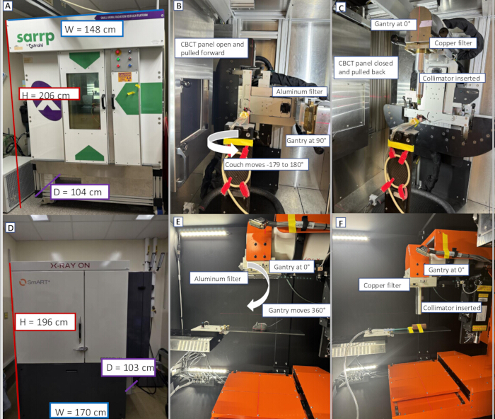
Figure 1: System configurations of System 1 and System 2. Panels (A–C) show System 1, and panels (D–F) show System 2. (A,D) Exterior views of each platform with annotated dimensions (height, width, and depth). (B,E) The internal configuration during imaging, including the couch rotation (B) and gantry rotation (E). An anesthetized mouse is shown in System 1 (B), and a mouse phantom is shown in System 2 (E). (C,F) The internal configuration during treatment delivery, highlighting the treatment setup with the collimation hardware in place in each system. Please click here to view a larger version of this figure.

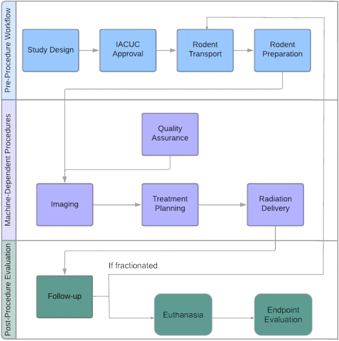
Figure 2: The flowchart summarizes the end-to-end experimental workflow, grouped into pre-procedure activities, machine-dependent procedures, and post-procedure evaluation. Arrows indicate the procedural sequence of the workflow. Please click here to view a larger version of this figure.

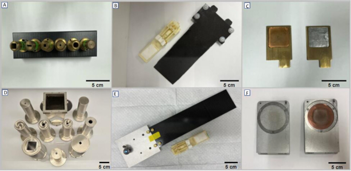
Figure 3: Materials used for treatment setup. Panels (A–C) show System 1 components, and panels (D–F) show System 2 components. (A,D) Collimator set in assorted sizes and shapes. (B,E) Animal support couch/bed used for imaging and treatment positioning. (C,F) Al and Cu filters. Please click here to view a larger version of this figure.

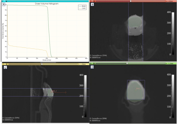
Figure 4: System 1 plan evaluation views. (A) Dose–volume histogram (DVH) for a whole brain treatment plan. The target (green line) is the whole brain, and the OAR (yellow line) is the upper spinal cord. (B) Axial (transverse) view of the calculated dose distribution overlaid on the imaging dataset. (C) Sagittal view of the calculated dose distribution. (D) Coronal view of the calculated dose distribution. The brain is contoured in green, and the beam edges are outlined in purple (B–D). Please click here to view a larger version of this figure.

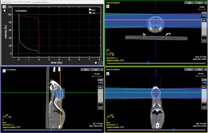
Figure 5: System 2 plan evaluation views. (A) Dose–volume histogram (DVH) for a whole brain treatment plan. The target (red line) is the brain, and the OAR (white line) is the upper spinal cord. (B) Axial dose view in the vertical × lateral plane. (C) Sagittal dose view in the vertical × longitudinal plane. (D) Coronal dose view in the lateral × longitudinal plane. The beam trajectory is shown in blue (B–D). Please click here to view a larger version of this figure.

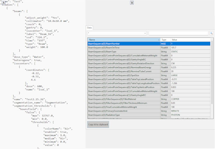
Figure 6: Treatment log files for System 2 and System 1. (A) System 1 log file reporting analogous treatment and beam-delivery information. (B) System 2 log file documenting treatment parameters. Please click here to view a larger version of this figure.

Table 1: Summary of key physical and operational specifications for System 1 and System 2 systems.Please click here to download this Table.

Discussion

The field of radiotherapy is evolving rapidly, and although there are numerous ongoing clinical trials, reproducible and accurate preclinical experiments are critical in understanding the radiobiological mechanisms that produce the desired end goal. Methods for small animal irradiation with fixed sources and total body irradiation may result in unwanted toxicity²⁰. The emergence of image-guided small animal irradiators allows for reproducible targeting and lower doses to OARs. This simulates parameters similar to patient treatments and allows for exploration of biological mechanisms with much lower risk of animal toxicity and death prior to the completion of the treatment regimen and reaching the desired endpoints. The use of small animal models in basic and preclinical studies has become a fundamental research model prior to clinical translation. Due to the small field-of-view and detector size, small animal irradiator systems can achieve sub-mm spatial accuracy superior to or on par with that of therapeutic linear accelerators²¹. Further, radiation therapy machines in oncology clinics are reserved for patient treatments during business hours, limiting the available time for preclinical animal studies. In this context, small animal irradiators provide researchers with a dedicated platform to perform radiobiological studies without interrupting the clinical workflow.

Both System 1 and System 2 allow image-guided small animal irradiation with high precision and sub-mm accuracy²². While there are similarities in the overall workflow of both systems, critical differences between the systems include the acquisition techniques used for CBCT, the beam quality, and the dose rate.

In both systems, the imaging prior to planning is performed using an Al filter and without beam collimation hardware, while treatment beam delivery is performed using a Cu filter and through dedicated beam shaping hardware. As such, caution must be exercised to ensure that the correct beam collimation hardware and filter are used for each task. The filters in System 2 are equipped with built-in sensors that communicate with the software and display which one is in place. This feature is absent from System 1, and there is no interlock for irradiation if the wrong filter is inserted.

For treatment planning, the System 1 software has the ability to utilize a previous plan as a template and calculate new beam irradiation times based on the newly acquired CT scan. This is absent from System 2 and requires new plan building for each scan or using the parameters from a previous plan, necessitating a balance between accuracy and throughput. For both machines, one of the steps with the largest uncertainty is manual contouring and should be performed with caution to ensure spatial accuracy of the dose to the desired region. The treatment planning dose calculations assume machine consistency, and for both machines, regular quality assurance procedures should be performed to evaluate output consistency. If the output has deviated by more than the allowed tolerance, the vendor company should be contacted to recalibrate as necessary. Quality assurance is performed based on vendor and institutional recommendations.

For each animal, required manual steps include switching the aluminum and copper filters between imaging and treatment, adding or switching the collimator, aligning the animal, irradiation, and removing the animal. Currently, there is no report on using automated tools for either system to perform these previously mentioned steps. In System 1, the CBCT panel must also be opened or closed and moved between imaging and treatment. As mentioned previously, if the protocol allows for a larger accuracy margin, certain steps may be omitted for efficiency. If using a previous or generic treatment plan, treatment planning may be omitted. For either machine, one operator is sufficient. However, workflow efficiency can be increased with additional personnel. For example, one user may focus on controlling the machine and switching out the filter and collimator while the other user tracks the anesthetization and switches the subjects out.

For both machines, one potential problem is the possibility of gantry collision with the couch because a collision can affect the isocenter alignment and requires recommissioning. Because of this, both machines are equipped with a camera that should be monitored whenever the gantry is in motion. If the user suspects that the gantry may collide with the couch, the operator should press the X-ray off button in the control software immediately. If the system does not respond, or if there is danger to the operator or subject, the operator should press the physical red emergency stop button. This will terminate all system power. The user should then reset the button and restart the system. Since the subject was partially irradiated, the operator should consult with the principal investigator to determine the best course for the subject.

Another potential problem is incorrect irradiation if the wrong filter or collimator is inserted. Although this is ideally avoided by checking the setup before each subject’s irradiation, because attaching the filter and collimator are manual steps and must occur between imaging and treatment, incorrect irradiation is possible. The subject number should be noted and reported to the principal investigator for monitoring. A final common problem is an OAR receiving too high a dose during treatment planning. Similar to clinical plans, modifications should be made to beam parameters, including adding additional beams at differing angles or switching to a dynamic plan. The subject position on the couch can also be adjusted.

Both systems have comparable CBCT imaging resolution and the ability for micro-CT, fluoroscopy, and bioluminescence imaging, which were not covered in this protocol. System 1 has a motorized variable collimator, a specialized collimation system that allows for conformal and non-coplanar irradiation, while System 2 has an automated adjustable collimator that creates rotatable rectangular fields. For treatment planning, System 1 can be used with Software 3, SmART-XPS, or micro-Raystation. System 2 is compatible with Software 6 or micro-Raystation.

The protocol described here is well-suited for systematic radiobiological research with small animal irradiator systems at conventional dose rates with spatially uniform fields. This protocol did not cover spatially fractionated radiation therapy (SFRT) and ultra-high dose rate (UHDR) RT because these two machines are not designed for such studies²³. The System 1 vendor company has developed a dedicated preclinical FLASH research platform with ongoing work on validating the system for UHDR studies²⁴. The System 2 vendor company has also developed a new cabinet system for conventional and UHDR delivery. Some authors have worked on building novel collimators for SFRT and changing the SSD to increase the dose rate^25,26,27. Future applications on the current systems include evaluating maximum dose rate capabilities at decreased SSD and dosimetric comparisons between the two machines using the same treatment plan. Further work may also include evaluating physical system constraints on other small animal models, such as rabbits.

Materials

List of materials used in this article

Name	Company	Catalog Number	Comments
MuriPlan v3.0.0	Software 3	Xstrahl	MuriPlan
MuriSlice v3.2.6	Software 2	Xstrahl	MuriSlice
PilotXRadConsole v1.30.3.5	Software 4	Precision X-Ray	PilotXRadConsole
SARRP Control Software v4.3.1	Software 1	Xstrahl	SARRP CS
Small Animal Radiation Research Platform	System 1	Xstrahl	SARRP
Small Animal Radiation Therapy Systems	System 2	Precision X-Ray	SmART+
SmART+ v1.30.3.5	Software 5	Precision X-Ray	SmART+
SmART-Advanced Treatment Planning v24.1.3.240826	Software 6	Precision X-Ray	SmART-ATP

References

- Bray F, et al. Global cancer statistics 2022: GLOBOCAN estimates of incidence and mortality worldwide for 36 cancers in 185 countries. CA Cancer J Clin. 2024;74(3):229-263.
- Miller KD, et al. Cancer treatment and survivorship statistics, 2022. CA Cancer J Clin. 2022;72(5):409-436.
- Atun R, et al. Expanding global access to radiotherapy. Lancet Oncol. 2015;16(10):1153-1186.
- Verhaegen F, Granton P, Tryggestad E. Small animal radiotherapy research platforms. Phys Med Biol. 2011;56(12):R55-R83.
- Tillner F, Thute P, Bütof R, Krause M, Enghardt W. Preclinical research in small animals using radiotherapy technology: a bidirectional translational approach. Z Med Phys. 2014;24(4):335-351.
- Pidikiti R, et al. Dosimetric characterization of an image-guided stereotactic small animal irradiator. Phys Med Biol. 2011;56(8):2585-2599.
- Brown KH, et al. A scoping review of small animal image-guided radiotherapy research: advances, impact and future opportunities in translational radiobiology. Clin Transl Radiat Oncol. 2022;34:112-119.
- Wong J, et al. High-resolution, small animal radiation research platform with X-ray tomographic guidance capabilities. Int J Radiat Oncol Biol Phys. 2008;71(5):1591-1599.
- Verhaegen F, van Hoof S, Granton PV, Trani D. A review of treatment planning for precision image-guided photon beam preclinical animal radiation studies. Z Med Phys. 2014;24(4):323-334.
- Foray N, Bourguignon M, Hamada N. Individual response to ionizing radiation. Mutat Res Rev Mutat Res. 2016;770(Pt B):369-386.
- Hall EJ, Giaccia AJ. Radiobiology for the Radiologist. 8th ed. Philadelphia (PA): Lippincott Williams & Wilkins; 2018.
- Bolcaen J, et al. MRI-guided 3D conformal arc micro-irradiation of a F98 glioblastoma rat model using the Small Animal Radiation Research Platform (SARRP). J Neurooncol. 2014;120(2):257-266.
- Yoon SW, et al. A precision 3D conformal treatment technique in rats: application to whole-brain radiotherapy with hippocampal avoidance. Med Phys. 2017;44(11):6008-6017.
- Chiver I, et al. Effects of the depletion of neural progenitors by focal X-ray irradiation on song production and perception in canaries. Sci Rep. 2023;13(1).
- Kampfer S, Duda MA, Dobiasch S, Combs SE, Wilkens JJ. A comprehensive and efficient quality assurance program for an image-guided small animal irradiation system. Z Med Phys. 2022;32(3):261-272.
- Seitzman BA, et al. Functional network disorganization and cognitive decline following fractionated whole-brain radiation in mice. GeroScience. 2024;46:543-562.
- LeMoyne Habimana-Griffin, et al. A novel focal duodenal radiation injury model reveals dose-, time-, and spatially dependent microbiome perturbations after radiation injury. Int J Radiat Oncol Biol Phys. 2026;125(2):590-602.
- Matinfar M, Ford E, Iordachita I, Wong J, Kazanzides P. Image-guided small animal radiation research platform: calibration of treatment beam alignment. Phys Med Biol. 2009;54(4):891-905.
- Ross RB, et al. PPARα agonism enhances immune response to radiotherapy while dietary oleic acid results in counteraction. Clin Cancer Res. 2024;30(9).
- Ghita M, Brown KH, Kelada OJ, Graves EE, Butterworth KT. Integrating small animal irradiators with functional imaging for advanced preclinical radiotherapy research. Cancers (Basel). 2019;11(2):170.
- Pokhrel D, Mallory R, Bernard ME. The spatial accuracy of ring-mounted Halcyon linac versus C-arm TrueBeam linac for single-isocenter/multi-target SBRT treatment. Med Dosim. 2023;48(3):170-175.
- Ghaznavi H, Rezaee M, Reynoso F, Darafsheh A. Emerging strategies in radiation therapy: promises and challenges of spatial fractionation, ultra-high dose rates, and nanoparticles. J Phys D Appl Phys. 2025;58(41):413002.
- Tajik Mansoury MA, Sforza D, Wong J, Iordachita I, Rezaee M. Dosimetric commissioning of small animal FLASH radiation research platform. Phys Med Biol. 2025;70(11):115015.
- Sharma S, et al. Advanced small animal conformal radiation therapy device. Technol Cancer Res Treat. 2016;16(1):45-56.
- Sayler E, Dolney D, Avery S, Koch C. Shielding considerations for the Small Animal Radiation Research Platform (SARRP). Health Phys. 2013;104(5):471-480.
- Hill MA, et al. The development of technology for effective respiratory-gated irradiation using an image-guided small animal irradiator. Radiat Res. 2017;188(3):247-257.
Reprints and Permissions
This article has been published
Video Coming Soon