Spatiotemporal Analysis of Coupled Thermo–Photoelastic Fields in Anisotropic Fiber-Reinforced Silicon Using an Eigenvalue Method

Summary

This study analyzes coupled thermo–photoelastic fields in anisotropic fiber-reinforced silicon using a normal mode and eigenvalue method. Results show spatial decay and time-dependent field evolution, with strong sensitivity to anisotropy. Heatmaps illustrate field distribution and localization.

Abstract

This study investigates a coupled thermo–photoelastic system in an anisotropic fiber-reinforced silicon semiconductor medium, aiming to capture the interaction between thermal, carrier, and mechanical fields. Such anisotropic fiber-reinforced materials play a crucial role in modern engineering applications, including microelectronic and optoelectronic devices, laser-based technologies, sensors, and advanced composite structures, where directional properties and enhanced mechanical performance are required. They are particularly important in the design of semiconductor components subjected to thermal and optical loading, where accurate prediction of coupled field behavior is essential for reliability and performance optimization. The governing equations are formulated based on the coupled physical model and subsequently transformed into a dimensionless form to simplify the analysis and highlight the relative influence of the involved parameters. The problem is solved using a normal mode technique and reduced to a first-order vector-matrix differential system, followed by an eigenvalue approach to obtain analytical solutions satisfying the imposed boundary conditions within a semi-infinite domain. Numerical analysis is carried out to examine the effect of time variation on all physical fields, revealing strong spatial attenuation and coupled behavior governed by anisotropy and fiber reinforcement. Spatiotemporal heatmap representations are used to visualize the evolution and localization of the fields, providing physical insight into the multiphysical interactions and demonstrating the effectiveness of the analytical approach.

Introduction

Thermo–photoelasticity has emerged as an important multidisciplinary field that describes the interaction between thermal, mechanical, and optical effects in semiconductor materials under photothermal excitation. The coupling between these fields becomes particularly notable in modern applications involving laser heating and optical excitation. For instance, Saeed¹ investigated thermo–photoelastic interactions in semiconductors using hyperbolic two-temperature models, demonstrating the importance of thermal relaxation effects in accurately predicting system behavior. The thermomechanical response of fiber-reinforced composites has also attracted considerable attention due to their enhanced mechanical strength and anisotropic properties. Li and Lambros² analyzed the dynamic thermomechanical behavior of such composites, highlighting their suitability for advanced engineering applications. Similarly, Kalkal et al.³ studied two-dimensional (2D) deformations in rotating functionally graded fiber-reinforced media under magnetic fields, showing the strong influence of anisotropy and external effects on system response. Furthermore, Pitarresi et al.⁴ examined the role of macroscopic heterogeneity in thermoelastic behavior, emphasizing the need for accurate modeling of composite materials. Recent developments have extended these studies to semiconductor media with coupled multiphysical effects. Mondal et al.⁵ investigated wave propagation in reinforced semiconductors considering memory responses and magnetic fields, revealing complex coupled interactions. Experimental studies, such as those by Akai et al.⁶, have evaluated fatigue damage in fiber-reinforced composites using thermoelastic temperature variations, confirming their practical importance. In addition, micromechanical approaches have been employed to estimate effective thermoelastic properties, as demonstrated by Lu et al.⁷. The influence of external loading and environmental conditions has also been widely studied. Barak and Dhankhar⁸ analyzed inclined loading in functionally graded fiber-reinforced media, while Kundu and Kalkal⁹ examined photothermal interactions under gravity and moving thermal loads. Chaudhary et al.¹⁰ investigated temperature-dependent properties using dual-phase-lag models, and Pandit et al.¹¹ applied fractional-order strain models to capture nonlocal deformation behavior. These studies highlight the importance of considering realistic loading and material conditions in thermoelastic analysis.

Dynamic and vibration-related phenomena have also been explored in semiconductor systems. Song et al.¹² studied photothermal vibrations in semiconductor structures, while Mondal and Sur¹³ analyzed wave propagation in orthotropic media with memory effects. Viscoelastic and microstructural effects have been considered by Abouelregal et al.¹⁴, and ramp-type heating effects have been investigated by Hobiny et al.¹⁵. Moreover, generalized thermoelastic models such as the three-phase-lag theory have been developed by Zenkour¹⁶ to improve prediction accuracy. Advanced multiphysical models incorporating electromagnetic and micropolar effects have further enhanced the understanding of thermo–photoelastic behavior. Al-Hazaemh et al.¹⁷ studied photo-electro-magneto-thermoelastic excitation in rotating semiconductor media, while Nazir and Kumar¹⁸ analyzed micropolar thermoelastic interactions. Song et al.¹⁹ also examined non-dissipative thermoelastic interactions, and Nasr and Abouelregal²⁰ investigated light absorption processes in semiconductors with cavities. Nonlocal and fractional-order models have played a crucial role in recent developments. Gupta et al.²¹ studied photothermal excitation in nonlocal porous media, while Hobiny and Abbas²² analyzed fractional-order wave propagation in semiconductors. Hafed and Zenkour²³ investigated inclined loading effects, and Oliinyk et al.²⁴ examined nonstationary thermo–photoelastic effects. Functionally graded semiconductor behavior under laser excitation was also explored by Awwad et al.²⁵, while Gupta et al.²⁶ investigated thermo-piezo-photoelectric coupling with memory-dependent models. Classical experimental approaches combining thermal and optical techniques have been established by Greene and Patterson²⁷ and Barone and Patterson²⁸, providing reliable methods for stress analysis. Furthermore, Kaur and Singh²⁹ developed nonlocal memory-dependent models for semiconductor resonators, and Abbas et al.³⁰ analyzed photothermal interactions with variable thermal conductivity. Experimental and numerical investigations of reinforced composite membranes were conducted by Lu et al.³¹, while Purkait and Kanori³² studied memory responses in rotating fiber-reinforced media. Abo-Dahab et al.³³ further examined wave reflection in fiber-reinforced thermoelastic media under loading conditions. More recently, advanced fractional and nonlocal thermoelastic models have been proposed to describe complex materials. Abouelregal et al.³⁴ investigated thermal responses in biological tissues using fractional models, while Selvamani et al.^35,36 studied nonlocal wave propagation and vibration behavior in nanobeams. Additionally, dual-phase-lag and viscoelastic models have been applied to microstructures by Abouelregal et al.³⁷, and fractional thermoelastic formulations with memory kernels have been developed^38,39 to capture complex coupled phenomena.

Despite these extensive developments, most existing studies primarily focus on analytical or numerical solutions without providing detailed spatiotemporal visualization of the physical fields. In many practical applications, especially in anisotropic fiber-reinforced semiconductor media, the system response strongly depends on both spatial and temporal variations, making visualization essential for accurate interpretation. Moreover, although numerical and experimental approaches provide valuable insights, analytical methods based on normal mode and eigenvalue techniques offer significant advantages in problems involving semi-infinite domains and coupled multiphysical systems. These approaches enable closed-form solutions, providing deeper physical understanding of wave propagation, attenuation, and coupling mechanisms, and serve as reliable benchmarks for validating numerical and experimental results.

In the present work, a comprehensive investigation of the coupled thermo–photoelastic behavior in an anisotropic fiber-reinforced semiconductor medium is presented. The novelty of this study lies in integrating an eigenvalue-based analytical approach with spatiotemporal heatmap visualization to provide deeper insight into the evolution and localization of physical fields. The aim of this work is to analyze the influence of anisotropy and fiber reinforcement on the interaction between thermal, mechanical, and carrier fields, and to demonstrate the applicability of the proposed method in interpreting complex multiphysical phenomena relevant to modern engineering applications such as semiconductor devices, sensors, and laser-based technologies.

Protocol

This study is based entirely on theoretical modeling and numerical simulations and does not involve human participants, animal subjects, or biological specimens. Therefore, ethical approval and informed consent were not required.

Mathematical Formulation of Photo-Thermoelasticity in Fiber-Reinforced Anisotropic Media
The present study considered a 2D fiber-reinforced anisotropic semiconductor half-space subjected to surface optical excitation. The medium occupied the region x ≥ 0, where the boundary at x = 0 represents the exposed surface. The coordinate system was defined such that the x-axis extended into the medium, while the y-axis lay along the surface and described the in-plane behavior. The material was assumed to be homogeneous but anisotropic because of the presence of aligned reinforcing fibers, which introduced directional dependence in the elastic and coupling properties. Optical absorption at the surface generated localized heating and excess charge carriers, leading to a fully coupled interaction between thermal, mechanical, and carrier fields. Accordingly, the state of the system was described by the temperature θ(x, y, t) (K), carrier density N (x, y, t) (m^-3), and displacement components u (x, y, t) and v (x, y, t)(m), under the assumption of small deformations. A schematic of the physical domain, coordinate system, fiber orientation, and applied optical excitation is illustrated in Figure 1. All symbolic and numerical computations were performed using Wolfram Mathematica (Version 12.0).

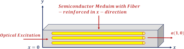
Figure 1. Schematic representation of the semi-infinite fiber-reinforced semiconductor medium subjected to optical excitation at the boundary x = 0. The coordinate system (x, y) is shown, with the fiber orientation aligned along the x-direction (a = (1, 0)), illustrating the geometric configuration and direction-dependent anisotropy of the medium. Please click here to view a larger version of this figure.

The constitutive relation for the stress tensor in a fiber-reinforced anisotropic thermoelastic semiconductor medium was expressed in the general form using Equation 1^1,5. In this formulation, θ denotes the temperature increment relative to the reference temperature T₀, while T represents the absolute temperature where applicable.

.   (1)

Here, C_ijkl are the elastic stiffness coefficients, e_kl is the strain tensor, and β_ij and η_ij represent the thermoelastic and carrier coupling tensors, respectively. In the presence of fiber reinforcement, the material response became direction-dependent and was governed by the fiber orientation vector a = (a_i), which introduced anisotropic contributions into both the elastic and coupling terms. Accordingly, the constitutive relation was expanded to explicitly incorporate the effect of fiber reinforcement as^2,3:

. (2)

Here, λ and μ_τ are the Lamé constants, and μ_L is the longitudinal shear modulus along the fiber direction. The parameter α represents fiber reinforcement effects and is distinct from α_ij, which denote thermal expansion coefficients. The unit vector defined the fiber orientation and introduced directional dependence in the stress–strain response. For the present 2D formulation, the fibers were assumed to be aligned along the x-axis; therefore, the orientation vector was explicitly taken as a = (1, 0). This specification provided a clear parametrization of the fiber direction and ensured that the anisotropic contributions were consistently incorporated into the governing equations, directly addressing the directional behavior induced by fiber reinforcement. For the present 2D configuration, the governing stress components reduced to:

, (3)

, (4)

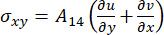. (5)

These equations illustrate the combined influence of anisotropy, fiber reinforcement, and multiphysical coupling effects. The coefficients β_ij and η_ij were defined in terms of the material parameters as follows:

,

,

,

.

Here, the coefficients A_ij represent the effective elastic constants of the fiber-reinforced anisotropic medium and were defined as follows:

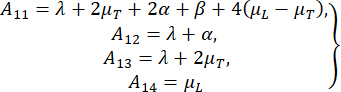. (6)

Here, λ, μ_L, and μ_T are the elastic constants of the anisotropic fiber-reinforced medium, while α_ij and ξ_ij represent the thermal and carrier expansion coefficients, respectively. The propagation of elastic waves in thermo–photoelastic semiconductor media was governed by the principle of conservation of linear momentum, which formed the foundation of dynamic thermoelastic analysis. In the absence of body forces, the general equation of motion for a deformable continuum is expressed as follows based on^1,15:

. (7)

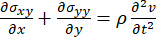
Here, ρ is the mass density and σ_ij is the stress tensor. In the present study, the formulation was restricted to a 2D configuration in the x - y plane, and the displacement field was represented by u(x, y, t) and v(x, y, t). Following standard formulations in thermo–photoelastic media, the governing equations of motion in two dimensions were written as follows:

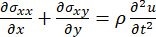, (8)

. (9)

Substituting the anisotropic fiber-reinforced constitutive relations into the above equations, the resulting coupled system of partial differential equations (DEs) was obtained as follows:

, (10)

. (11)

Here, subscripts denote partial differentiation with respect to spatial and temporal variables. These equations highlight the coupled influence of anisotropy, fiber reinforcement, temperature gradients, and carrier diffusion on the dynamic response of the medium. In the presence of optical excitation, the thermal field inside the semiconductor was strongly influenced by the interaction with carrier density and mechanical deformation, resulting in a fully coupled energy transport process. Unlike classical heat conduction, the temperature evolution in such media was governed by additional source terms arising from carrier recombination and thermoelastic effects, which significantly altered the heat propagation characteristics. The heat conduction equation in the framework of generalized thermoelasticity was expressed as follows^16,20:

. (12)

Here, C_E is the specific heat at constant strain, representing the thermal capacity of the material, and T₀ denotes the reference absolute temperature of the medium in its equilibrium state. For the present 2D configuration, this equation reduced to^16,20:

. (13)

This equation demonstrates that the temperature field was affected not only by directional thermal conductivity but also by carrier recombination through the term , as well as by time-dependent deformation through the thermoelastic coupling terms. This formulation captured the essential multiphysical interactions governing heat transfer in the anisotropic fiber-reinforced semiconductor and highlighted the role of both carrier dynamics and mechanical response in modifying the thermal behavior of the system. When a semiconductor medium was subjected to optical excitation, a significant number of charge carriers were generated due to the absorption of incident radiation. These carriers underwent transport processes that included spatial diffusion, recombination, and thermally driven generation, all of which were inherently linked to the temperature field within the material. Consequently, the carrier density became one of the key variables governing the coupled thermo–photoelastic response.

In the present formulation, the evolution of the carrier concentration was described through a balance between diffusion mechanisms, decay effects, and thermal activation processes, leading to the following governing relation^1,5”

. (14)

Here, D_E represents the carrier diffusion coefficient and  is the 2D Laplacian operator in the x - y plane. The term  accounts for recombination effects with relaxation time τ, while k is the thermo-carrier coupling coefficient defined as , which characterizes the sensitivity of the equilibrium carrier concentration N₀ to temperature variations. This relation highlights the role of temperature as a driving mechanism for carrier generation and establishes a direct coupling between the thermal and electronic fields in the anisotropic fiber-reinforced semiconductor medium.

The governing equations and mathematical formulation of the coupled photothermoelastic carrier system have been established. The physical and material parameters corresponding to the silicon (Si) medium are summarized in Table 1, along with their numerical values, units, and corresponding references. These parameters are subsequently used in the numerical computations and in the nondimensionalization process.

Symbol	Value	Unit	Reference
λ	3.64 × 10¹⁰	N/m²	12
μT	5.46 × 10¹⁰	N/m²	12
μL	3.20 × 10¹⁰	N/m²	12
ρ	2330	kg/m³	13
CE	695	J/(kg·K)	30
k11	0.0921 × 10³	W/(m·K)	30
k22	0.0963 × 10³	W/(m·K)	30
DE	2.5 × 10⁻³	m²/s	22
τ	5 × 10⁻⁵	s	15
T₀	300	K	15
Eg	1.11 × 10⁻¹⁹	J	12
α11	3.1 × 10⁻⁶	K⁻¹	30
α22	3.5 × 10⁻⁶	K⁻¹	30
ξ11	−7 × 10⁻³¹	m³	21
ξ22	−9 × 10⁻³¹	m³	21
κ	2.16 × 10²¹	m⁻³·s⁻¹·K⁻¹	21
α	−1.28 × 10¹⁰	N/m²	28
β	220.90 × 10¹⁰	N/m²	28
ω	2.95 + 1i	s⁻¹	12
a	1	— (dimensionless)	13
y	0.6	m	13
θ₀	1	— (dimensionless)	15
N₀	1	— (dimensionless)	15

Table 1. Material properties and parameters used in the numerical analysis of the anisotropic fiber-reinforced semiconductor medium. All quantities are expressed in SI units unless otherwise specified. Dimensionless parameters are indicated accordingly. The listed values correspond to silicon-based material properties and model parameters employed in the present computations, as obtained from the cited references. The thermo-carrier coupling coefficient κ is defined as κ = (∂N₀/∂T)(1/τ), following standard formulations in thermo–photoelastic semiconductor models.

Non-Dimensional Formulation of the Coupled Anisotropic Photo–Thermoelastic Model
To simplify the governing equations and obtain a consistent nondimensional representation of the coupled thermo–photoelastic system, appropriate characteristic scales were introduced for the spatial coordinates x,y, time t, displacement components u, v, temperature T, carrier density N, and stress σ. These scaling parameters were selected consistently based on the intrinsic physical properties of the medium and the coupling mechanisms between thermal, mechanical, and carrier fields, following established formulations reported in the literature^16,21. Accordingly, the dimensionless variables were defined as follows:

, , , , , , , , , .

This transformation reduced the number of independent material parameters and provided a normalized representation of the coupled system. By substituting the above dimensionless variables into the previously derived governing equations, the system was rewritten in nondimensional form. For simplicity, the prime notation associated with the dimensionless variables was subsequently omitted. This procedure yielded a compact set of dimensionless partial DEs, which can be written in the following form:

, (15)

, (16)

, (17)

. (18)

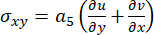
After applying the nondimensional transformation, the stress components of the system were written in the following normalized form:

, (19)

, (20)

. (21)

The dimensionless parameters a_i were introduced to represent compact combinations of the physical and material properties governing the coupled anisotropic photo–thermoelastic behavior. Each coefficient reflected a specific interaction mechanism within the system and provided insight into the relative influence of the underlying physical processes.  represents the ratio between normal coupling stiffness and the principal elastic stiffness, reflecting the degree of anisotropic interaction between the two displacement components.  characterizes the relative contribution of transverse deformation to the normal stress component.  measures the directional variation of thermoelastic coupling, indicating anisotropy in thermal expansion effects.  describes the anisotropic influence of carrier density on the induced elastic deformation.  represents the normalized shear stiffness and quantifies the contribution of shear deformation relative to normal deformation.  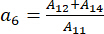accounts for the combined coupling between normal and shear deformation in the governing displacement equations.  expresses the ratio between transverse stiffness and shear stiffness, highlighting anisotropic deformation behavior.  represents the normalized inertial parameter, relating wave propagation effects to shear stiffness.  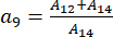characterizes the coupling between displacement gradients in different spatial directions.  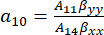quantifies the relative contribution of thermal effects to the displacement field in the transverse direction.  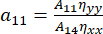measures the effect of carrier-induced deformation relative to shear stiffness.  : represents the anisotropy in thermal conductivity along different spatial directions.  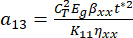characterizes the influence of carrier recombination on heat generation within the medium.  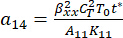represents the coupling between thermal effects and time-dependent elastic deformation.  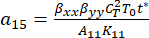accounts for the combined influence of anisotropic thermal expansion in both spatial directions.  represents the normalized diffusion parameter controlling the rate of carrier transport.  characterizes the relative strength of carrier recombination effects.  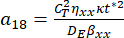describes the coupling between thermal variations and carrier generation processes.

Analytical Solution Using the Normal Mode Technique
To obtain analytical solutions for the coupled anisotropic thermo–photoelastic system, the normal mode technique was employed due to its effectiveness in reducing the governing partial DEs into a more tractable system of ordinary DEs. This approach is widely used in the analysis of wave propagation phenomena, including dispersion and attenuation. Accordingly, harmonic variations of the field variables in both time and the transverse spatial direction were assumed^1,12,23. Thus, the displacement components, temperature, carrier density, and stress were expressed in exponential form as follows:

. (22)

Here, ω denotes the complex frequency governing the temporal behavior of the fields, while a represents the wave number associated with the spatial variation along the y-direction. These parameters were selected to satisfy stability requirements and ensure physically admissible bounded solutions within the semi-infinite domain. By substituting the above assumed forms into the previously derived nondimensional governing equations and simplifying the resulting expressions, the original coupled system of partial DEs was reduced to a system of ordinary DEs with respect to the spatial coordinate , which can be written as follows:

, (23)

, (24)

, (25)

. (26)

Furthermore, the corresponding stress components in the transformed domain were written as follows:

, (27)

, (28)

. (29)

Here, D denotes the differential operator . These equations represent the reduced form of the governing system in the normal mode domain and provide the basis for deriving the characteristic equation and constructing the general analytical solution in subsequent steps. The coefficients were defined as follows: , , , , , , , , , .

Matrix DE Formulation and Eigenvalue Analysis
Following the application of the normal mode transformation, the governing system given in Equations 23–26 was reduced to a set of second-order ordinary DEs with respect to the spatial coordinate . To facilitate a systematic solution, this system was converted into an equivalent first-order system by introducing auxiliary variables corresponding to the first derivatives of the field quantities. Specifically, the following variables were defined:

, . (30)

Using these definitions, Equations 23–26 were rewritten as the following system of eight first-order DEs:

, (31)

, (32)

, (33)

, (34)

. (35)

The above system was expressed in compact matrix A form as follows:

. (36)

The state vector was given by following:

. (37)

and the system matrix took the explicit form:

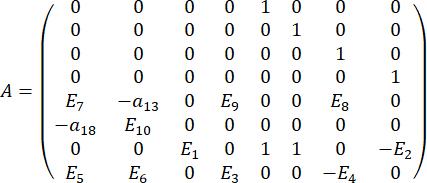. (38)

This formulation transformed the original system into an eigenvalue problem^1,15. The characteristic equation was obtained from

. (39)

which yields an eighth-order polynomial governing the eigenvalues. In a reduced form, the characteristic polynomial can be written as

. (40)

where Z_i the coefficients are functions of the system parameters and are defined explicitly below. The resulting eigenvalues determine the spatial behavior of the solution, including attenuation and propagation characteristics. Only eigenvalues satisfying Re(m) > 0 are retained to ensure physically admissible solutions that decay exponentially as x → ∞.

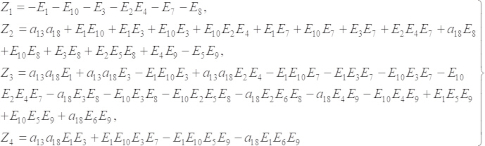. (41)

The roots of the characteristic polynomial define the eigenvalues m, which govern the spatial behavior of the solution. These eigenvalues were computed numerically using Mathematica by constructing the characteristic polynomial via the CharacteristicPolynomial function and solving the resulting algebraic equation using NSolve. Since the problem is formulated in a semi-infinite domain (x ≥ 0), only physically admissible solutions that remain bounded as x → ∞ are considered. Accordingly, only eigenvalues satisfying Re(m) > 0 were retained, ensuring exponentially decaying solutions of the form exp(−mx) as x → ∞. The remaining roots were discarded as they correspond to non-decaying or unbounded solutions that are not consistent with the physical requirements of the model.

For each retained eigenvalue m, the corresponding eigenvector was obtained from the associated algebraic system

, (42)

and was expressed in the following form:

. (43)

Expanding the above matrix equation, the following system of linear equations was obtained:

, (44)

, (45)

, (46)

, (47)

. (48)

Due to the homogeneity of the eigenvalue problem, the eigenvectors were defined up to an arbitrary multiplicative constant. To obtain a unique and consistent representation, a normalization condition was imposed by fixing one component of the eigenvector. In the present work, the first component was selected such that q₁ = 1, and the remaining components were determined sequentially from the above system of equations. From a computational perspective, this normalization was implemented by assigning a unit value to one component and solving the resulting system of linear equations to evaluate the remaining components. This procedure provided a systematic and reproducible way to compute the eigenvectors associated with each admissible eigenvalue.

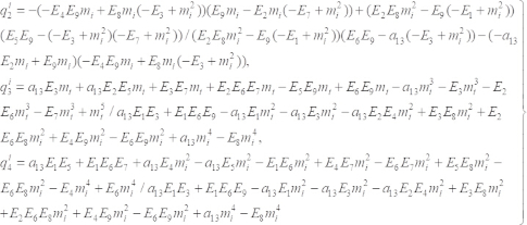. (49)

And the remaining components follow accordingly from the system relations. These eigenvectors describe the relative contributions of temperature, carrier density, and displacement fields within each mode. Consequently, the general solution of the problem was constructed as a linear combination of the admissible eigenmodes, each associated with an eigenvalue and its corresponding eigenvector, thereby providing a complete analytical description of the coupled anisotropic photo–thermoelastic behavior in the half-space medium. The general solution of the system was therefore written as follows:

. (50)

Here, C_i are constants determined from the boundary conditions. By expanding the above vector expression, the field variables were obtained as follows:

, (51)

, (52)

, (53)

. (54)

This representation shows that the solution consists of a superposition of exponential modes, where each eigenvalue-eigenvector pair contributes independently to the overall physical response. The admissible eigenvalues are selected such that their real parts are positive, ensuring bounded and physically meaningful solutions as x → ∞.

Boundary Conditions and Physical Constraints
By substituting the general solution into the prescribed boundary conditions at x = 0, a system of linear algebraic equations in terms of the constants C_i was obtained. Specifically, each boundary condition (temperature, carrier density, and displacement constraints) was expressed in terms of the eigenmode expansions, resulting in a set of equations relating the coefficients C_i. This procedure led to a linear system that can be written in matrix form as BC = D, where B is the coefficient matrix constructed from the components of the eigenvectors evaluated at the boundary, C = (C₁, C₂, C₃,C₄)^T is the vector of unknown constants, and is determined from the imposed boundary values such as θ₀, N₀, and the displacement constraints. The resulting linear system was solved computationally using Mathematica, where the coefficient matrix and right-hand side vector were assembled explicitly, and the unknown constants were obtained using the LinearSolve routine. These constants were then substituted back into the general solution to construct the complete expressions for the physical fields, which were subsequently used in the numerical evaluation and graphical representation of the results.

The imposed boundary conditions were given as follows:

Temperature constraint:

. (55)

This condition represents a harmonically varying surface temperature induced by periodic optical heating. It acts as the primary thermal excitation driving the coupled thermoelastic and carrier transport processes within the medium. The amplitude θ₀ characterizes the intensity of the applied thermal load.

Carrier density constraint:

. (56)

This boundary condition describes the photo-generated carrier density resulting from optical illumination. It reflects the electronic excitation due to photon absorption and its harmonic modulation consistent with the incident optical field.

Displacement constraint:

. (57)

This condition indicates that the boundary is mechanically constrained in the transverse direction. Hence, no displacement occurs along the v-direction at the surface.

Shear stress constraint:

. (58)

This condition corresponds to a traction-free boundary with respect to shear stress. It ensures that no tangential forces act on the surface, which is consistent with a mechanically free boundary in the tangential direction. In addition to the boundary conditions at x = 0, the physical requirement at infinity was imposed as:  ensuring bounded physical solutions within the semi-infinite domain. Before presenting the numerical results, the overall computational procedure adopted in this study is summarized in Figure 2. The numerical values of the excitation parameters θ₀, N₀, complex frequency ω, and wave number a used in the computations are listed in Table 1. Parameters listed in Table 1 include both dimensional material constants and nondimensional parameters used in the normalized formulation. For numerical evaluation, the spatial domain was defined as , the transverse coordinate was fixed at y = 0.6, and the temporal domain was considered within . These ranges were used for all numerical computations and graphical representations.

Figure 2. Computational workflow of the proposed method. The figure illustrates the sequence of steps from formulation to numerical results: governing equations, nondimensionalization, application of the normal mode technique, conversion to a first-order system, matrix formulation, eigenvalue and eigenvector analysis, application of boundary conditions, determination of constants, and generation of numerical plots. Please click here to view a larger version of this figure.

Results

Numerical Results
In this section, numerical computations were performed to analyze the behavior of the coupled thermo–photoelastic-carrier system in an anisotropic fiber-reinforced semiconductor medium. The material considered was silicon (Si), and its physical and material parameters are listed in Table 1. These material constants were directly substituted into the governing equations and implemented in the numerical computations to evaluate the field variables. All parameters were...

Discussion

The obtained results provide clear physical insight into the coupled thermo–photoelastic behavior in anisotropic fiber-reinforced semiconductor media. The present study proposes an eigenvalue-based analytical framework for investigating the interaction between thermal loading, carrier generation, and elastic deformation in such media. The observed response is fundamentally governed by the strong coupling between these physical processes. The absorption of optical energy at the boundary leads to localized heating an...

Materials

List of materials used in this article

Name	Company	Catalog Number	Comments
Computational software (symbolic and numerical analysis)	Wolfram Research	Wolfram Mathematica (Version 12.0) was used	Used for eigenvalue computation, analytical solution implementation, and numerical evaluation
Data visualization tools (contour and heatmap generation)	Wolfram Research	Wolfram Mathematica (Version 12.0) was used for generating 2D contour plots and spatiotemporal heatmaps	Used for generating 2D contour plots and spatiotemporal heatmaps
Material parameter dataset (silicon semiconductor properties)	Various literature sources	N/A	Physical constants (elastic, thermal, carrier-related) used in computations (Table 1)
Personal computer/workstation	HP	N/A	Computations were performed on a standard personal computer running Windows OS with sufficient memory for numerical simulations
Equation editor	Microsoft  Word and MathType	N/A	Used for formatting and presenting mathematical expressions in the manuscript
Reference management software	Elsevier	N/A	Used for managing references and formatting citations (Vancouver style)