Land Urbanization, Ecological Planning, and Carbon Stock Dynamics in Xinjiang, China, Using an Integrated Geospatial Modeling Workflow

Summary

An integrated geospatial modeling workflow quantifies land urbanization and carbon stock dynamics. Built-up land expansion is associated with carbon stock loss and negative spatial spillover effects, whereas ecological planning scenarios retain high-carbon land and support coordinated low-carbon governance.

Abstract

This study developed and applied an integrated workflow that combined remote sensing, land-use simulation, ecosystem-service assessment, and spatial econometric methods to quantify the influence of land urbanization and ecological planning on carbon stock dynamics in the Xinjiang Uygur Autonomous Region of northwestern China. Using land-use/land-cover, impervious-surface, nighttime-light, vegetation, topographic, socioeconomic, and planning-constraint data from 2000–2020, the workflow identified historical urbanization patterns, simulated four future planning scenarios, estimated carbon stock using the InVEST carbon module, and evaluated direct and spatial spillover effects using spatial econometric models. The results show that built-up expansion occurred primarily through cropland conversion and was accompanied by increases in impervious-surface coverage and nighttime light intensity. Simulation results indicate that the ecological protection scenario yields the highest carbon stock retention, whereas the natural development scenario results in the greatest carbon loss. Forest land was identified as the most vulnerable high-carbon land-use class, with a total carbon density of 144.9 Mg C/ha compared with 29.4 Mg C/ha for built-up land. Spatial Durbin model results show that land urbanization has a negative direct effect (−0.231) and indirect spillover effect (−0.117), yielding a total effect of −0.348 on carbon stock density, whereas ecological planning intensity has a positive total effect (+0.245). These findings support coordinated ecological planning across administrative boundaries to promote low-carbon regional development.

Introduction

Against the backdrop of global climate change and the transition toward low-carbon development, rapid urbanization has become a major driver of changes in regional land-cover patterns and biogeochemical cycles¹. As human activities continue to expand in scale and intensity, accelerated land urbanization in developing regions not only alters land-use patterns but also reshapes ecosystem structure and function. In essence, land urbanization involves the conversion of high-carbon-density natural vegetation into low-carbon-density artificial surfaces, resulting in substantial losses of regional carbon storage capacity². For rapidly developing regions, balancing economic growth with the protection of ecological space has become a critical challenge in territorial spatial planning. Traditional land-use studies have primarily focused on patterns of physical expansion while often overlooking the dynamic interactions between spatial development and carbon-cycle processes³. Consequently, there is a need for integrated analytical approaches that quantify the effects of land urbanization on carbon stock dynamics and provide a scientific basis for ecological protection and low-carbon governance.

Recent advances in remote sensing and geographic information systems have substantially improved land-use change modeling and ecosystem-service assessment^4,5. Multi-scenario land-use simulation coupled with ecological accounting has become a widely used approach for evaluating the environmental consequences of urban expansion⁶. In particular, Patch-generating Land Use Simulation (PLUS) and Integrated Valuation of Ecosystem Services and Tradeoffs (InVEST) models have been applied to quantify how planning constraints influence land-use trajectories and carbon-stock outcomes^{7,8,9,10,11,12}. Related ecosystem-service studies have further demonstrated that land-cover change, urban development policies, and ecological protection measures can alter water yield, carbon sequestration, soil retention, and ecosystem-service trade-offs across rapidly urbanizing landscapes^{13,14,15,16,17}. However, most previous studies have focused on land-use conversion and ecosystem-service outputs, with less attention given to how socioeconomic development pressures generate spatially dependent carbon-stock responses among neighboring administrative units.

Three key gaps motivate the present workflow. First, previous PLUS–InVEST applications often treat study areas as closed physical systems and do not explicitly evaluate whether the effects of land urbanization spill over into adjacent units. Second, validation, uncertainty, and sensitivity analyses are frequently reported only briefly, making it difficult to determine whether scenario rankings remain stable under alternative land-use simulation parameters, carbon-pool coefficients, and spatial-weight specifications. Third, spatial econometric studies often identify associations between development intensity and ecological outcomes without linking these relationships to remote sensing observations, future land-use scenarios, and carbon stock accounting. An integrated workflow is therefore needed to connect observation, scenario simulation, carbon accounting, and spatial-mechanism identification within a reproducible analytical framework.

Accordingly, this study establishes a reproducible analytical workflow that integrates remote sensing, PLUS-based scenario simulation, InVEST carbon-stock assessment, and spatial econometric analysis. Focusing on the Xinjiang Uygur Autonomous Region in northwestern China, the study evaluates historical land-urbanization patterns from 2000–2020, examines how alternative planning scenarios influence future land-use configurations, quantifies the resulting effects on carbon-stock distribution, and investigates the direct and spatial spillover effects of land urbanization, ecological planning intensity, vegetation condition, and socioeconomic factors on carbon-stock dynamics. The principal contribution of this workflow is the integration of scenario-based forecasting with mechanism identification to support ecological redline delineation, compact-growth planning, cross-boundary carbon compensation, and low-carbon regional governance.

Protocol

Publicly available geospatial, remote-sensing, planning, and aggregated socioeconomic datasets were used in this study. No human participants, animal subjects, clinical materials, or identifiable personal information were involved. Institutional ethics approval was therefore not required. The specific software environments, computational packages (including spatial econometric and high-resolution visualization libraries), dataset Digital Object Identifiers (DOIs), and source URLs for all resources necessary to reproduce this workflow are detailed in the comprehensive Table of Materials.

1. Study area and analytical framework

The analysis was conducted in the Xinjiang Uygur Autonomous Region, northwestern China, with a specific analytical focus on the delineated urban extents of key cities (Figure 1) to accurately capture localized expansion dynamics. This boundary was used consistently for raster clipping, land-use simulation, carbon-stock assessment, and administrative-unit aggregation. The analytical sample size (n) comprised 105 county-level administrative units analyzed across three discrete temporal nodes (2000, 2010, and 2020), with land-use simulations incorporating 50 stochastic replicates to capture spatial uncertainty.

A multi-scale analytical framework integrating grid-level and administrative-unit analyses was employed. At the grid scale, land-use/land-cover data, nighttime light intensity, impervious surface coverage, vegetation indices, topographic variables, and ecological planning constraints were used to identify land urbanization patterns, simulate future land-use scenarios, and evaluate carbon stock distribution. At the administrative-unit scale, socioeconomic, transportation, and environmental variables were incorporated into spatial econometric analyses to assess the direct and spillover effects of land urbanization and ecological planning on carbon-stock dynamics.

The analytical framework comprised five components. First, multi-temporal remote-sensing and land-use data were used to characterize spatiotemporal patterns of land urbanization, including built-up land expansion, development intensity, and land-use restructuring. Second, ecological protection, cropland protection, and low-carbon planning scenarios were developed to simulate future land-use patterns. Third, the InVEST carbon-storage module was used to quantify carbon-stock distribution and change under historical and future land-use conditions. Fourth, global and local spatial autocorrelation analyses were conducted to identify clustering patterns and hotspot regions associated with carbon-stock variation. Fifth, spatial econometric models were used to evaluate the magnitude, direction, and spillover effects of land urbanization, ecological-planning intensity, and environmental and socioeconomic drivers on carbon-stock dynamics.

Figure 1 presents the overall analytical workflow. The workflow links study-area definition, multi-source data integration, land-urbanization identification, ecological-planning scenario development, land-use simulation, carbon-stock assessment, spatial autocorrelation analysis, and spatial econometric modeling. Multi-source spatial data served as the input layer. Land-urbanization identification and historical land-use analysis formed the pattern-characterization layer. Ecological planning scenarios and carbon stock assessment formed the prediction and impact evaluation layer. Spatial autocorrelation and econometric analyses were used to identify spatial mechanisms and support policy interpretation.

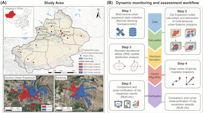
Figure 1: Study area, data integration, and technical workflow. (A) Multi-scalar spatial context and precise urban analytical boundaries for key cities in the Xinjiang Uygur Autonomous Region, northwestern China. (B) Integrated technical workflow linking multi-source spatial data, remote sensing-based land urbanization identification, ecological planning scenario design, PLUS land-use simulation, InVEST carbon stock assessment, spatial autocorrelation, hotspot analysis, and spatial econometric modeling. ND = natural development; EP = ecological protection; CP = cropland protection; LC = low-carbon optimization; OLS = ordinary least squares; SAR = spatial autoregressive model; SEM = spatial error model; SDM = spatial Durbin model. Please click here to view a larger version of this figure.

2. Data sources and variable system

A multi-source dataset was compiled to support land-urbanization identification, ecological-planning scenario simulation, carbon-stock assessment, and spatial econometric analysis. The dataset included land-use/land-cover data, impervious-surface fraction, nighttime light intensity, normalized difference vegetation index (NDVI), topographic variables, transportation accessibility indicators, hydrological variables, population density, gross domestic product (GDP) density, planning constraints, climate variables, and carbon pool parameters. Table 1 summarizes the dataset category, variable description, unit, spatial and temporal resolution, source, and analytical application. Key datasets were obtained for 2000, 2010, and 2020. Land-use and major remote-sensing products were harmonized to resolutions ranging from 30 m to 1 km, depending on analytical requirements.

Table 1: Data sources and variable system. The table reports dataset category, variable, description, unit, spatial/temporal resolution, source, and analytical use for land urbanization identification, scenario simulation, InVEST carbon stock accounting, and spatial econometric modeling. NDVI = normalized difference vegetation index; DEM = digital elevation model; LULC = land use/land cover. Please click here to download this Table.

All spatial layers were projected to a common coordinate system, clipped to the study-area boundary shown in Figure 1, and resampled or aggregated to the required grid or administrative-unit scale. Missing values were screened before spatial overlay analysis. Raster datasets used in PLUS and InVEST analyses were aligned at the pixel level, whereas socioeconomic variables were aggregated to administrative units for spatial regression. This preprocessing workflow ensured consistent spatial units and comparable time points across temporal analyses, scenario simulations, carbon-stock calculations, and econometric modeling.

Land-use/land-cover data served as the primary input for historical change detection and future land-use simulation. Original land-use categories were reclassified into six classes: arable land, forest land, grassland, water bodies, built-up land, and unused land. This classification scheme was used consistently for land-use change analysis, scenario development, and InVEST carbon-stock calculations. The built-up land proportion, impervious surface coverage, and nighttime light intensity were used as indicators of land urbanization. Impervious-surface coverage and nighttime-light intensity served as remote-sensing proxies for development intensity and human activity. NDVI was included as an ecological indicator in subsequent spatial econometric analyses.

Topographic and location variables included elevation, slope, distance to major roads, road density, and proximity to major rivers. These variables were used as drivers in land-use simulation and as control variables in spatial econometric models. Together, they represented terrain constraints, transportation accessibility, and hydrological connectivity.

Socioeconomic variables included population density and GDP density, supplemented by road-network density where available. These variables were used to characterize development intensity and human activity pressures associated with changes in carbon stocks. The variable framework integrated indicators of land development, socioeconomic pressure, and ecological context to represent the multiple factors influencing carbon-stock dynamics.

An ecological-planning intensity index was developed using ecological redlines, nature reserves, water-body buffer zones, slope-restriction areas, and other environmentally sensitive regions. This index served both as a constraint layer in future land-use simulations and as an explanatory variable in spatial econometric analyses.

For InVEST carbon-stock assessment, four carbon-pool parameters were compiled for each land-use class: aboveground biomass carbon, belowground biomass carbon, soil organic carbon, and dead organic matter carbon. Parameter values were obtained from published regional studies, InVEST guidance documents, and local land-cover characteristics and were mapped to the unified land-use classification system. Carbon stock refers to the total estimated carbon contained within these four pools, whereas carbon-stock density refers to carbon stock per unit area.

Variables were grouped into three categories. The first category comprised land-urbanization indicators, including the proportion of built-up land, impervious-surface coverage, and nighttime light intensity. The second category included ecological and planning variables, such as NDVI, ecological-planning intensity, elevation, slope, and hydrological proximity. The third category comprised socioeconomic drivers, including population density, GDP density, and road density. These variables were used to evaluate the relationships among land urbanization, ecological planning, and carbon-stock dynamics.

3. Remote sensing-based identification of land urbanization

The spatiotemporal patterns of land urbanization were identified using three complementary indicators: built-up land expansion, impervious-surface coverage, and nighttime light intensity. Built-up land expansion was extracted from sequential land-use maps to delineate the physical extent and progression of urban development from core built-up areas to surrounding regions. Impervious-surface coverage was calculated to quantify development intensity at the grid level, while nighttime light intensity raster data were processed and normalized to represent human activity and functional concentration. These spatial layers were subsequently integrated to construct the historical land-urbanization dataset. The combined indicators were used to identify areas of sustained development intensification, transition zones, and relatively stable regions, and to evaluate the spatial correspondence between physical land development and functional urbanization.

A land-use transition matrix was constructed to quantify the magnitude and direction of land-use conversion among arable land, forest land, grassland, water bodies, construction land, and unused land. Particular attention was given to transitions from ecological and agricultural land classes to construction land. The matrix was used to identify dominant conversion pathways and the principal source land classes contributing to urban expansion.

Landscape-pattern analysis was conducted to evaluate structural changes associated with land urbanization. Metrics included patch density, edge density, landscape shape index, and fragmentation-related indicators. These metrics were calculated for each study period and used to quantify changes in landscape configuration, spatial continuity, and fragmentation associated with the expansion of built-up land.

4. Ecological planning scenario design and land-use simulation

Future land-use patterns were simulated using the Patch-generating Land Use Simulation (PLUS) model under four planning scenarios: natural development (ND), ecological protection (EP), cropland protection (CP), and low-carbon optimization (LC). Scenario assumptions, land-conversion rules, restricted land types, and expected carbon-stock outcomes are summarized in Table 2.

Table 2: Scenario control rules and transition constraints. The table defines land conversion probabilities and spatial constraints for natural development (ND), ecological protection (EP), cropland protection (CP), and low-carbon optimization (LC) scenarios. Notes: Scenario abbreviations strictly correspond to those utilized in the PLUS modeling and Results sections. The scenario settings define policy-oriented conversion rules and restricted land types used in the simulations; all statutory exclusion zones remained non-convertible in the final spatial layers. Please click here to download this Table.

Historical land-use maps and spatial driver variables were integrated into the PLUS model to estimate baseline land-transition probabilities using the cellular automata (CA) module. For the ecological protection (EP), cropland protection (CP), and low-carbon optimization (LC) scenarios, ecological redlines, permanent basic cropland, water-body buffers, and other planning constraints were incorporated as spatial restriction layers to limit land conversion in accordance with the predefined scenario rules. Target land-demand quantities for 2030 were subsequently defined for each scenario, and the CA module was executed using 50 stochastic replicates to generate the final land-use projections.

Land-use simulation was performed using the PLUS model and its cellular automata (CA) framework with multi-type stochastic patch generation. Historical land-use maps and environmental and socioeconomic driver variables were used to estimate land-expansion probabilities for each land-use class. Future land-demand quantities were then specified according to the requirements of each planning scenario, and corresponding land-use maps were generated for the target simulation period.

Model performance was evaluated through historical back-casting prior to future simulation. Earlier land-use maps and associated driver variables were used to simulate a later observed land-use map. Agreement between simulated and observed land-use distributions was assessed using overall accuracy (OA), the Kappa coefficient, and the Figure of Merit (FoM). Validation was conducted at both the overall level and by major land-use class. Historical back-casting from 2010 to 2020 yielded an overall accuracy (OA) of 93.4%, a Kappa coefficient of 0.89, and a Figure of Merit (FoM) of 0.26, indicating a highly reliable capacity for spatial projection in subsequent multi-scenario simulations.

Uncertainty and sensitivity analyses were conducted to evaluate the robustness of simulation outcomes. PLUS sensitivity analyses examined the effects of alternative transition-resistance settings and neighborhood-weight parameters for major land-use classes. InVEST sensitivity analyses evaluated the influence of variation in carbon-pool coefficients across land-use types. Spatial econometric sensitivity analyses compared alternative spatial-weight matrix specifications. These analyses were used to assess whether scenario rankings and the direction of the principal urbanization and ecological-planning effects remained consistent under alternative parameter settings. Specifically, outcome stability was rigorously confirmed: scenario rankings and the negative spatial spillover effects of land urbanization remained invariant when transition-resistance parameters and carbon-pool coefficients were perturbed by ±15%.

5. Carbon stock assessment

Carbon stock was assessed using the InVEST carbon model. Baseline parameters for the four carbon pools (aboveground biomass, belowground biomass, soil organic carbon, and dead organic matter) were assigned to each reclassified land-use type using the biophysical values summarized in Table 3. Historical land-use maps (2000–2020) and PLUS-simulated future land-use raster datasets were then imported into the model and integrated with the corresponding carbon-density parameters. The model was subsequently executed to estimate total regional carbon stock (Tg C), grid-level carbon-stock density (Mg C/ha), and spatial maps of carbon-stock change (ΔC) for the historical and future scenarios.

Reclassified land-use maps were linked to the corresponding baseline carbon-pool parameter values reported in Table 3. The sensitivity of carbon stock estimates to parameter uncertainties was tested by adjusting these baseline values by ±15%, with detailed sensitivity outcomes. The model was used to calculate total carbon stock, carbon-stock density, and carbon-stock change for each land-use class under historical conditions and future planning scenarios.

Three categories of outputs were evaluated. First, total regional carbon stock and temporal trends were calculated to quantify the magnitude and direction of carbon-stock change over time. Second, spatial distributions of carbon stock and carbon-stock change were mapped to identify areas of carbon retention and carbon loss. Third, carbon-stock estimates were compared across planning scenarios to evaluate the relative effects of ecological protection, cropland protection, and low-carbon optimization strategies on carbon-stock conservation.

Table 3: Baseline carbon-pool parameters for different land-use types. The table reports aboveground biomass carbon, belowground biomass carbon, soil organic carbon, dead organic matter carbon, and total carbon density used in the InVEST carbon stock module. Units are Mg C/ha. Notes: Values represent baseline parameters utilized in the InVEST model. Total carbon density equals the sum of the four carbon pools. Sensitivity analyses perturbing these baseline values by ±15% are reported in Table 6. Please click here to download this Table.

6. Spatial autocorrelation and spatial econometric analysis

Spatial autocorrelation analysis was conducted to determine whether carbon stock and carbon-stock change exhibited significant spatial dependence. Global Moran's I was calculated to evaluate the overall degree of spatial clustering in carbon-stock distribution and carbon-stock change across the study area. Local Moran's I was then used to identify local spatial association patterns, including high-high, low-low, high-low, and low-high clusters. Hotspot analysis was performed to identify areas of concentrated carbon loss and carbon-stock retention.

Spatial econometric models were used to examine the relationships between land urbanization, ecological planning, environmental conditions, socioeconomic factors, and carbon-stock dynamics. Carbon-stock density or carbon-stock change served as the dependent variable. Explanatory variables included the land urbanization index, built-up land proportion, ecological planning intensity, normalized difference vegetation index (NDVI), population density, GDP density, road density, elevation, slope, mean annual precipitation, and mean annual temperature.

Ordinary least squares (OLS) regression was used as the baseline model. Residual spatial dependence was evaluated before estimating the spatial autoregressive (SAR), spatial error (SEM), and spatial Durbin (SDM) models. Model performance and coefficient estimates were compared across specifications.

A row-standardized spatial-weight matrix was constructed to represent neighborhood relationships among administrative units. The primary specification was based on spatial contiguity, and robustness analyses compared alternative distance-based and nearest-neighbor spatial-weight matrices where available.

Direct, indirect, and total effects were calculated from the SDM to evaluate local and spatial spillover relationships. Terrain, accessibility, vegetation, climate, and socioeconomic variables were included as control variables to reduce omitted-variable bias. Model coefficients were interpreted as conditional spatial associations rather than definitive causal effects. Variables with p-values exceeding conventional significance thresholds were interpreted as weak or suggestive evidence and were not treated as statistically robust effects.

Results

Remote sensing-based identification of land urbanization
Based on multi-period remote sensing identification results, the study area experienced a significant intensification of land urbanization between 2000 and 2020, accompanied by the restructuring of land-use patterns and the reshaping of landscape configurations. Overall, the expansion of construction land demonstrated a concentric expansion pattern radiating from core urban areas to peripheral zones. Concurrent increases in human activity intensity and surface impermeability levels indicate that rapid development has not only altered the quantitative structure of land use but also profoundly reconfigured regional spatial organization patterns.

The land urbanization identification results, exemplified by the Urumqi representative subset in Figure 2A, clearly demonstrate the phased expansion trajectories of construction land use from 2000–2020. In 2000, construction land was primarily concentrated in central urban areas with relatively compact spatial configurations. By 2010, peripheral expansion had intensified significantly, forming transitional zones surrounding core areas. By 2020, construction land had exceeded the original compact boundaries, spreading in multiple directions and forming discrete expansion patches distant from core zones, reflecting typical outward expansion patterns and multi-center diffusion trends. Consistent with these expansion patterns, Figure 2B shows a significant central-to-peripheral gradient in impervious surface coverage within the study area by 2020. The highest values were observed in central urban areas and adjacent built-up regions, indicating that surface hardening intensity and development intensity were most pronounced in core functional zones. Although peripheral areas maintained relatively low overall coverage, multiple high-value patches emerged along transportation corridors and secondary urban nodes, demonstrating that impermeabilization had expanded beyond urban centers through development spillovers into surrounding areas. Figure 2C reveals that the regions with the largest increases in nighttime lighting intensity between 2000 and 2020 were predominantly concentrated in central urban areas, along major radial transportation axes extending outward, and at several peripheral growth nodes.

From a temporal perspective, Figure 2D further summarizes the consistent upward trends of the three land urbanization indicators between 2000 and 2020. To facilitate direct comparison across indicators with divergent intrinsic units and scales, the raw values of each indicator were standardized using a min-max normalization approach, scaling them to a uniform 0–1 range:

Following this normalization procedure, the proportion of built-up areas maintained the highest relative growth rate (with its raw regional mean increasing from 3.2% ± 1.4% SD in 2000 to 8.7% ± 3.1% SD in 2020), indicating that land development expansion served as the most direct spatial manifestation during this period. The proportion of impervious surfaces increased rapidly (from 2.8% ± 1.2% SD in 2000 to 7.9% ± 2.8% SD in 2020), reflecting significant surface hardening associated with new development areas. Although nighttime lighting intensity started at a relatively low level, its growth became more pronounced later, indicating accelerated increases in human activity concentration and functional enhancement.

Figure 2: Spatiotemporal evolution patterns of land urbanization. (A) Phased expansion trajectories of construction land (2000–2020); (B) Spatial distribution of impervious surface coverage in 2020 (%); (C) Variations in nighttime light (NTL) intensity changes between 2000 and 2020 (nW/cm²/sr). (D) Temporal trends in the three core land urbanization indicators examined in this study (built-up area, impervious surface fraction, and nighttime light intensity). Trend lines represent the regional means of min-max-normalized index values (scaled from 0–1 for comparative visualization), calculated across all n = 105 county-level administrative units in the study area. Please click here to view a larger version of this figure.

The results of historical land-use changes further reveal the specific processes of land urbanization. The land-use transfer flow chart in Figure 3A indicates that the most significant land conversion during the study period was from cropland to construction land, the predominant trend among all major conversion pathways. While some forest land, grassland, and water bodies also underwent varying degrees of conversion, the overall pattern was dominated by cropland outflow. Concurrently, bidirectional flows were observed between cropland and forest land, as well as among grassland and other land types, indicating that, amid rapid development, land-use systems undergo multi-type reorganization driven by urban expansion rather than unidirectional evolution. However, analyzing the spatial distribution patterns and flow widths reveals that construction land remains the primary net inflow category, further confirming the dominant role of development expansion in the study area over the past two decades.

The matrix analysis in Figure 3B provides a more quantitative representation of land use conversion intensity across different time periods. High-value areas are predominantly concentrated in cropland-related conversion units, with the most significant conversion occurring from cropland to construction land, indicating that non-agricultural use of cropland is the primary manifestation of land-use change in the study area. A considerable proportion of construction land also maintains spatial continuity and stability within its boundaries, reflecting the sustained expansion of existing development zones while preserving strong spatial integrity. In contrast, while the conversion scale of forest land, grassland, and water bodies remains relatively small, localized encroachment by construction land on these ecological areas warrants attention.

At the landscape pattern level, Figure 3C shows a sustained increase in landscape indices across 2000, 2010, and 2020, with patch density, edge density, landscape shape index, and fragmentation index all peaking in 2020. This indicates that as urbanization advances, the study area's landscape structure has evolved from an initially relatively intact and well-defined pattern to a more fragmented, complex, and discontinuous spatial configuration. Notably, the rise in edge density and shape complexity quantitatively characterizes a more irregular and complex geometric configuration of the newly expanded construction land patches.

Figure 3: Historical land-use change and landscape pattern restructuring. (A) Sankey diagram illustrating the high-resolution land-use transition flows and primary conversion pathways between 2000 and 2020. (B) Land-use conversion matrix quantifying the spatial transition area among the six land-use classes (km²). (C) Radar chart depicting changes in key landscape indices (Patch Density, Edge Density, Landscape Shape Index, and Fragmentation Index) across the 2000, 2010, and 2020 periods. All labels and flow values have been scaled for optimal legibility. Please click here to view a larger version of this figure.

Ecological planning scenario design and land-use simulation
When combined with the scenario control rules established in Table 2, land-use simulation results under different ecological planning orientations show distinct differentiation patterns. The natural development scenario tends to sustain historical expansion inertia, while the ecological protection scenario emphasizes rigid constraints on ecological redlines and sensitive zones. The cropland protection scenario prioritizes maintaining spatial continuity of agriculture, whereas the low-carbon optimization scenario emphasizes balanced development between compact urbanization and ecological coordination. These findings indicate that variations in planning rules quantitatively alter the simulated area of newly added construction land and reconfigure the spatial distribution of ecological-agricultural patches across the four scenarios.

Focusing on the Urumqi representative subset, the spatial simulation results from the PLUS model indicate that the natural development scenario (ND) shown in Figure 4A exhibits the most pronounced trend in construction expansion. New construction land primarily extends outward from the periphery of existing built-up areas, forming broad expansion zones in multiple directions, indicating that urban growth remains predominantly lateral expansion under weak regulatory constraints. This expansion pattern directly encroaches on cropland and transitional ecological zones surrounding central urban areas, further fragmenting built-up boundaries. In contrast, the ecological protection scenario (EP) depicted in Figure 4B shows significantly reduced new construction land use, with expansion confined to a limited number of developable plots near central urban areas, while peripheral forestlands, aquatic corridors, and ecological buffer zones remain largely intact.

In terms of agricultural protection and development coordination, the cropland protection scenario (CP) depicted in Figure 4C exhibits spatial constraints distinct from those of the EP. Under this scenario, large peripheral croplands remain largely intact, with new construction activities concentrated primarily at the edges of existing built-up areas and localized development nodes, demonstrating expansion intensity intermediate between ND and EP. Conversely, the low-carbon optimization scenario (LC) shown in Figure 4D demonstrates a more compact growth pattern. New construction land does not spread extensively outward but is relatively concentrated along major development axes and the peripheries of existing built-up areas, exhibiting directional expansion boundaries and more regular spatial configurations.

Figure 4: Spatial distribution of PLUS-simulated future land-use patterns under differentiated ecological planning scenarios, illustrated using the Urumqi metropolitan subset. (A) Natural development scenario (ND) showing historical expansion inertia. (B) Ecological protection scenario (EP) emphasizing strict spatial constraints. (C) Cropland protection scenario (CP) prioritizing agricultural continuity. (D) Low-carbon optimization scenario (LC) reflecting compact growth patterns. Please click here to view a larger version of this figure.

Carbon stock assessment
Table 3 presents the baseline carbon density parameters across land-use types. Forest land recorded the highest total carbon density (144.9 Mg C/ha), primarily driven by soil organic carbon (94.5 Mg C/ha) and aboveground biomass (36.8 Mg C/ha). Grassland and cropland exhibited moderate total carbon densities of 88.9 Mg C/ha and 82.1 Mg C/ha, respectively. In contrast, artificial and non-vegetated surfaces yielded significantly lower values, with built-up land at 29.4 Mg C/ha and unused land at 19.7 Mg C/ha.

From the perspective of historical evolution patterns, Figure 5A demonstrates significant spatial reorganization of carbon stock in the study area between 2000, 2010, and 2020. In 2000, high-carbon density regions were primarily concentrated in peripheral ecological zones, exhibiting an overall pattern of higher concentrations at the periphery and lower values at the center. By 2010, the total regional carbon stock initially declined as urban expansion encroached on ecological spaces, although some localized peripheral areas temporarily maintained elevated carbon stock levels. By 2020, this downward trend accelerated significantly; the overall color gradient lightened, and high-value areas shrank notably, indicating a continuous and substantial depletion in regional total carbon stock and weakened spatial continuity of high-carbon patches.

As illustrated in Figure 5B, the ND scenario yielded the lowest median carbon density (72.4 Mg C/ha, IQR = 14.6 Mg C/ha). The EP and CP scenarios produced higher median densities of 86.8 Mg C/ha (IQR = 12.3 Mg C/ha) and 81.2 Mg C/ha (IQR = 15.8 Mg C/ha), respectively. The spatial distribution of carbon stock changes (ΔC) in Figure 5C indicates that carbon losses (negative ΔC) are geographically widespread under the ND scenario. Conversely, positive ΔC values are concentrated in peripheral ecological zones under the EP scenario, whereas the LC scenario exhibits a spatially heterogeneous distribution of localized carbon gains and losses.

Figure 5D further reveals the source composition of the total carbon stock and its changes across historical periods and future scenarios, from the perspective of land-use-type contribution structures. Both historical and projected phases consistently show that forest land and grassland remain the primary contributors to total carbon stock, followed by arable land, while construction land, water bodies, and unused land contribute relatively less. Future scenario comparisons indicate that the EP scenario achieves the highest total carbon stock, while the ND scenario shows the lowest, with CP and LC scenarios falling in between. This pattern aligns closely with the varying degrees of retention of high-carbon-density ecological land use across different scenarios.

Figure 5: Historical and scenario-based carbon stock dynamics. (A) Spatial distribution of total carbon stock (Tg C) and carbon stock density (Mg C/ha) in 2000, 2010, and 2020. (B) Violin plot of carbon density distribution (Mg C/ha) across different scenarios. (C) Spatial distribution of carbon stock changes (ΔC, Mg C/ha) under future scenarios relative to the 2020 baseline. (D) Contribution of different land use types to total carbon stock (Tg C). The violin plots visualize the probability density of carbon stock density (n = 105 administrative units per scenario). Inner thick horizontal lines indicate the median, and dashed lines represent the interquartile range (IQR). Asterisks in panel B denote the statistical significance of differences between the natural development (ND) baseline and other simulated scenarios, determined using the Kruskal-Wallis H test (* p < 0.05, ** p < 0.01, *** p < 0.001). Please click here to view a larger version of this figure.

Spatial autocorrelation and spatial econometric analysis
From the perspective of spatial aggregation patterns, Figure 6A reveals significant local spatial autocorrelation in carbon stock variations across the study area. High-high aggregation zones are predominantly concentrated in the central-northern core development belt, indicating that these regions and adjacent units generally exhibit co-directional carbon stock enhancement characteristics with strong spatial interconnectivity. Low-low aggregation zones are more prevalent in southern and peripheral regions, reflecting relatively low amplitudes of carbon stock variation and spatial stability. In contrast, high-low and low-high aggregation types are relatively limited, primarily occurring between core zones and peripheral transition zones, suggesting pronounced spatial misalignment and boundary transition phenomena in localized areas.

The hotspot analysis in Figure 6B further reveals the spatial polarization pattern of carbon stock changes. Significant hotspots are predominantly distributed across several units in the central and northeastern regions, indicating that these areas collectively experience high pressure for carbon loss and are sensitive zones with concentrated land development activities. In contrast, significant cold spots are concentrated in the western and southern regions, reflecting stronger carbon-stock retention capacity or lower development disturbance. Furthermore, the bivariate OLS regression analysis in Figure 6C reveals that larger increases in the urbanization index are associated with increasingly negative carbon stock change rates, indicating progressively greater carbon losses. This is consistent with the negative SDM coefficients reported in Table 4.

Figure 6: Spatial autocorrelation and coupling analysis of carbon stock. (A) Local Indicators of Spatial Association (LISA) patterns of carbon stock variations; the final Global Moran's I statistic and p-value are reported in the panel. (B) Hotspot and coldspot distribution of carbon stock changes. (C) Coupling relationship between the comprehensive land urbanization index and carbon stock change rate. The scatter plot displays a statistically significant negative correlation (Pearson's r = -0.612, R² = 0.375, p < 0.001), accompanied by the displayed OLS regression equation (y = -5.42× - 1.25) and a 95% confidence band, confirming the empirical relationship observed in the spatial models. LISA = Local Indicators of Spatial Association. Please click here to view a larger version of this figure.

Table 4: Estimation results of spatial econometric models. The table compares the results of ordinary least squares (OLS), spatial autoregressive (SAR), spatial error (SEM), and spatial Durbin (SDM) models for the effects of urbanization, ecological planning, vegetation, socioeconomic, accessibility, terrain, and climate variables on carbon stock density. P-values are reported in parentheses. Notes: P-values are reported in parentheses. Significance levels: *p < 0.05, **p < 0.01, *** p < 0.001. All spatial econometric models (SAR, SEM, SDM) were estimated using a row-standardized Queen contiguity spatial-weight matrix based on a balanced panel of n = 105 county-level units over 3 periods (Total N = 315 observations). Please click here to download this Table.

The measurement results presented in Table 4 demonstrate that spatial models outperform the OLS benchmark, indicating spatial dependence in carbon stock dynamics and supporting the use of spatial econometric models. The land urbanization index has a negative SDM direct effect (−0.231, p = 0.008), indirect effect (−0.117, p = 0.041), and total effect (−0.348, p = 0.001), suggesting that increased development intensity is associated with lower carbon stock density both locally and in neighboring units. Built-up land proportion, road density, elevation, slope, NDVI, and ecological planning intensity show statistically meaningful effects at conventional levels in at least one model component. GDP density, by contrast, has a weak negative total effect (−0.132, p = 0.083) and non-significant direct and indirect effects; therefore, it is interpreted as suggestive rather than robust evidence.

The cross-model coefficient comparison in Figure 7A indicates that the land urbanization index and ecological planning intensity retain consistent signs across the OLS, SAR, SEM, and SDM specifications, whereas the magnitudes and significance of some control variables vary across models. As detailed in Figure 7B, C, the SDM results indicate that the land urbanization index exerts a significant negative direct effect (-0.231, p = 0.008) and a negative indirect spillover effect (-0.117, p = 0.041) on carbon stock density, resulting in a total effect of -0.348 (p = 0.001). Conversely, ecological planning intensity demonstrates positive direct (0.149, p = 0.021) and indirect (0.096, p = 0.038) effects, yielding a total effect of 0.245 (p = 0.005) (Table 5 and Table 6). Furthermore, the interaction analysis in Figure 7D illustrates the moderating effect: the negative slope of the marginal effect curve between the urbanization index and carbon stock density flattens significantly at higher levels of ecological planning intensity (upper 95% CI bound).

Figure 7: Driving mechanisms and spatial spillover effects. (A) Cross-model coefficient comparison for core explanatory variables. Error bars represent the 95% confidence intervals (CI) of the standardized coefficients. (B) Decomposition of direct, indirect, and total effects of land urbanization and ecological planning. (C) Empirical spatial distribution of the local indirect spillover effects of land urbanization across the 105 county-level units in Xinjiang. (D) Moderating effect of ecological planning intensity on the relationship between urbanization and carbon stock density (Mg C/ha), with the shaded regions indicating the 95% CI. SAR = spatial autoregressive model; SEM = spatial error model; SDM = spatial Durbin model. Significance symbols in panel B indicate the p-values of the estimated coefficients and marginal effects, derived from the z-statistics of the respective spatial econometric models (* p < 0.05, ** p < 0.01, *** p < 0.001). Please click here to view a larger version of this figure.

Table 5: Model performance and validation metrics for PLUS land-use simulation (2010–2020 back-casting). Metrics were calculated by comparing the actual 2020 land-use map with the 2020 land-use map simulated using 2010 baseline data. An overall Kappa > 0.80 and FoM > 0.20 indicate substantial agreement and high reliability for spatial projections. Please click here to download this Table.

Table 6: Sensitivity and robustness analysis of the integrated workflow. Key parameters for the PLUS simulation, InVEST carbon assessment, and spatial econometric analyses were varied to evaluate the robustness of model outputs. The table summarizes the parameter tested, perturbation range or alternative specification, observed impact on the primary outcomes, and the resulting stability assessment. Please click here to download this Table.

DATA AVAILABILITY:
The processed computational materials supporting this study, including the tabulated data underlying the quantitative analyses and selected figures, the PLUS model configuration parameters, the InVEST carbon-pool parameter table, and the spatial econometric scripts, have been deposited in the Zenodo repository (https://zenodo.org/records/21159171). The deposited computational materials are sufficient to reproduce the statistical analyses and quantitative results presented in this study.

Discussion

This study presents an integrated analytical workflow that combines remote sensing-based land urbanization identification, PLUS multi-scenario land-use simulation, InVEST-based carbon stock assessment, and spatial econometric modeling to analyze the relationships among land urbanization, ecological planning, and carbon stock dynamics in Xinjiang, northwestern China. Rather than treating these components as separate technical exercises, the workflow links observed land conversion, future planning alternatives, carbon-pool consequences, and spatial spillover mechanisms in a single reproducible sequence.

The spatiotemporal analysis reveals that land urbanization in the study area followed a centrifugal expansion trajectory from 2000–2020, transitioning from compact, core-area growth toward multi-directional, polycentric sprawl. This pattern aligns with the broader urbanization literature documenting leapfrog development in rapidly industrializing regions, where infrastructure investment and economic agglomeration simultaneously push development boundaries outward. Critically, the dominant land conversion pathway—cropland to built-up land—confirms that agricultural land continues to bear the heaviest burden of urban encroachment, a finding consistent with studies on peri-urban land dynamics in China and other developing economies. However, unlike the highly integrated megaregions in eastern China, urbanization in Xinjiang is strictly constrained by oasis boundaries and water availability. Consequently, this encroachment disproportionately threatens the limited arable land and ecological transition zones adjacent to vital hydrological corridors, making the local carbon-cycle processes inherently more vulnerable to development disturbances. The concurrent rise in impervious surface fraction and nighttime light intensity further suggests that physical expansion and functional intensification are advancing in tandem, implying that land urbanization in this context encompasses not merely a real growth but a deepening structural transformation of the regional landscape².

The scenario simulation results demonstrate that ecological planning orientation exerts substantial influence over the spatial configuration of future land use, and by extension, over regional carbon stock outcomes¹⁸. The natural development scenario produces the steepest carbon losses, driven by unconstrained outward expansion into high-carbon-density ecological land. In contrast, the ecological protection scenario retains the highest carbon stock levels by enforcing strict spatial exclusions around forests, wetlands, and river buffers¹⁹. The low-carbon optimization scenario, while not matching the ecological protection scenario in absolute carbon stock retention, achieves a more balanced outcome by concentrating growth along existing development corridors and away from ecologically sensitive areas. These differential outcomes underscore a fundamental planning trade-off: the intensity and spatial targeting of ecological constraints directly determine how much carbon capital a rapidly developing region can preserve amid growth pressures^20,21.

The carbon stock parameters further reinforce this interpretation. The substantial disparity in carbon sequestration capacity between natural ecological spaces and artificial surfaces signifies that each unit of forested area lost to urban conversion represents a disproportionately large carbon liability. The persistent dominance of forest and grassland in the regional carbon budget, combined with their documented vulnerability to built-up encroachment, positions ecological land protection as a cornerstone of any low-carbon spatial governance strategy³.

The spatial econometric results extend the remote sensing and InVEST findings by showing that carbon-stock losses are not only local land-cover consequences. The SDM results indicate that land urbanization exerts a significant negative direct effect on local carbon stock density, coupled with a pronounced negative indirect spillover effect on neighboring administrative units. The negative indirect effect of land urbanization can be interpreted through three plausible cross-boundary mechanisms. First, development pressure may be displaced from highly regulated or saturated core units into adjacent cropland and ecological transition zones. Second, transport corridors and industrial chains can transmit land-development demand beyond a single administrative boundary, producing carbon-stock losses in neighboring units. Third, fragmentation of ecological corridors can reduce the continuity of high-carbon land and weaken the surrounding carbon stock capacity. Conversely, ecological planning intensity demonstrates a robust positive overall impact, indicating that stringent planning constraints not only buffer carbon-stock loss locally but also synergistically enhance regional carbon-stock retention when ecological spatial governance is coordinated across administrative boundaries^22,23.

Policy applications
The results have direct applications for territorial spatial planning. First, ecological redline and river-buffer policies should prioritize high-carbon forest and grassland patches because their conversion produces disproportionately large carbon-stock losses. Second, compact growth and transport-oriented development controls can reduce outward encroachment on cropland and ecological transition zones. Third, carbon compensation and ecological restoration should be coordinated among neighboring units because the negative indirect effect indicates that one jurisdiction's development can affect surrounding carbon-stock conditions. Finally, the combined workflow can be used as a screening tool before land-use plan approval to compare carbon outcomes under alternative planning constraints.

Limitations
Several limitations should be acknowledged. Carbon-pool parameters remain partly literature-based and may not fully capture local heterogeneity in soil, vegetation, and management. Although sensitivity checks were used to test the stability of scenario rankings, field calibration would improve confidence in absolute carbon-stock estimates. The spatial econometric analysis reduces omitted-variable bias by including terrain, accessibility, vegetation, climate, and socioeconomic controls, but valid instrumental variables were unavailable; therefore, the coefficients should be interpreted as conditional spatial associations rather than definitive causal effects.

Future directions
Future work should integrate local biomass and soil-carbon measurements, finer-resolution socioeconomic data, formal instrumental-variable or quasi-experimental designs, and dynamic spatial panel models to further test causal pathways. Future applications should also report class-specific PLUS validation metrics, carbon-pool sensitivity ranges, and alternative spatial-weight results in supplementary tables to enable independent reproduction of scenario rankings and spillover estimates.

Conclusion
This study demonstrates that the remote sensing–PLUS–InVEST–spatial econometric workflow can identify land urbanization patterns, evaluate ecological planning scenarios, quantify carbon-stock consequences, and diagnose spatial spillover effects within one reproducible framework. The key findings demonstrate that historical built-up expansion was primarily driven by cropland conversion, accompanied by significant increases in surface impermeability and human activity intensity. Scenario simulations confirm that ecological protection strategies maximize regional carbon retention, whereas spatial econometric modeling establishes that land urbanization exerts both negative direct and spatial spillover effects on carbon stock dynamics. Ultimately, this integrated workflow provides a robust, reproducible analytical framework for quantifying the ecological trade-offs of urban expansion and offers a mechanism-driven diagnostic tool for spatial evaluation in ecologically fragile regions.

Materials

List of materials used in this article

Name	Company	Catalog Number	Comments
Custom Spatial Econometric Scripts and Output Datasets	Authors	Zenodo repository: https://zenodo.org/records/21159171	Used to reproduce the spatial econometric analyses and supporting computational workflow described in this study.
High-resolution Population Density Grids	WorldPop	https://www.worldpop.org/	Used as socioeconomic input data for spatial econometric analyses.
InVEST (Integrated Valuation of Ecosystem Services and Tradeoffs)	The Natural Capital Project, Stanford University	Version 3.14.0; https://naturalcapitalproject.stanford.edu/	Used to estimate carbon stock and carbon-stock changes under historical and simulated land-use scenarios.
Matplotlib & Pillow (Python Libraries)	Python Community	https://matplotlib.org/; https://python-pillow.org/	Used to generate publication-quality figures and process high-resolution (600 dpi) graphical outputs.
Multi-temporal Land-use/Land-cover Datasets	Resource and Environment Science and Data Center (RESDC), Chinese Academy of Sciences	https://www.resdc.cn/	Used as the primary input dataset for land-use change analysis and PLUS simulations.
PLUS (Patch-generating Land Use Simulation) model	High-performance Spatial Computational Intelligence Lab (HPSCIL)	https://github.com/HPSCIL/Patch-generating_Land_Use_Simulation_Model	Used to simulate future land-use patterns under multiple ecological planning scenarios.
PySAL (Python Spatial Analysis Library)	PySAL Developers	https://pysal.org/	Used to perform spatial autocorrelation analyses and spatial econometric modeling.
Python Programming Environment	Python Software Foundation	Version 3.9+; https://www.python.org/	Used for data preprocessing, spatial analysis, statistical calculations, and workflow implementation.
Topographic (DEM) and Remote Sensing Data	United States Geological Survey (USGS)	https://earthexplorer.usgs.gov/	Used to derive topographic variables and remote-sensing inputs for land urbanization analysis and model parameterization.

References

- Xiong Z, Zhang Y, Liu M. Assessing land urbanization and ecological planning impact on carbon stock and its economic value from coupled InVEST-PLUS models. Sci Rep. 2025;15:30494. https://doi.org/10.1038/s41598-025-30494-x
- Ge K, Zou S, Lu Y, Chen Y. Spatial effects and influence mechanisms of urban land use green transition on urban carbon emissions. Ecol Indic. 2025;172:113261. https://doi.org/10.1016/j.ecolind.2025.113261
- Li L, et al. Spatio-temporal evolution of land use and carbon stock under multiple scenarios based on the PLUS-InVEST model: A case study of Chengdu. Sustainability. 2025;17(21):9903. https://doi.org/10.3390/su17219903
- Wang Z, Zhong A, Wei E, Hu C. Carbon stock simulation and land use optimization for high-water-table resource-based cities based on the coupled GMOP-PLUS-InVEST model. Remote Sens. 2024;16(23):4480. https://doi.org/10.3390/rs16234480
- Liu Y, Mei X, Yue L. Response of carbon stock to land use change and multi-scenario predictions in Zunyi, China. Sci Rep. 2025;15:236. https://doi.org/10.1038/s41598-024-81735-8
- Sun G, Li Y, Huang R. Spatial and temporal evolution of carbon stocks in Yulin City under changing environments. Sci Rep. 2025;15:12219. https://doi.org/10.1038/s41598-025-12219-w
- Tang J, Peng W. Spatiotemporal dynamics and influencing factors of land carbon stock in Chengdu Plain using an integrated model. Sci Rep. 2025;15:11248. https://doi.org/10.1038/s41598-025-11248-x
- Wang Y, Zhang Z, Chen X. Land use transitions and the associated impacts on carbon stock in the Poyang Lake Basin, China. Remote Sens. 2023;15(11):2703. https://doi.org/10.3390/rs15112703
- Tao Y, Tian L, Wang C, Dai W. Dynamic simulation of land use and land cover and its effect on carbon stock in the Nanjing Metropolitan Circle under different development scenarios. Front Ecol Evol. 2023;11:1102015. https://doi.org/10.3389/fevo.2023.1102015
- Song M, Yu S, Qin H. Land-use/land-cover change and its impact on ecosystem carbon stock in Binhai New Area, Tianjin, China from 1985 to 2060. Environ Earth Sci. 2025;84:481. https://doi.org/10.1007/s12665-025-11728-x
- Liang X, et al. Understanding the drivers of sustainable land expansion using a patch-generating land use simulation (PLUS) model: A case study in Wuhan, China. Comput Environ Urban Syst. 2021;85:101569. https://doi.org/10.1016/j.compenvurbsys.2020.101569
- Sharp R, et al. InVEST 3.14.0 User's Guide. The Natural Capital Project; Stanford, CA; 2023. https://storage.googleapis.com/invest-users-guide/index.html
- Basha U, et al. Spatial-temporal assessment of annual water yield and impact of land use changes on Upper Ganga Basin, India, using InVEST model. J Hazard Toxic Radioact Waste. 2024;28(2). https://doi.org/10.1061/JHTRBP.HZENG-1188
- Deeksha, Shukla AK. Ecosystem services: A systematic literature review and future dimension in freshwater ecosystems. Appl Sci. 2022;12(17):8518. https://doi.org/10.3390/app12178518
- Shukla AK, Jain MK, Khare D, Mishra PK. Spatio-temporal assessment of annual water balance models for upper Ganga Basin. Hydrol Earth Syst Sci. 2018;22:5357-71.
- Nayak D, Shukla AK, Devi NR. Decadal changes in land use and land cover: Impacts and their influence on urban ecosystem services. Aqua Water Infrastruct Ecosyst Soc. 2024;73(1):57-72.
- Nayak D, Shukla AK. Assessing ecosystem service trade-offs and synergies in the rapidly urbanizing coastal region of Mangaluru Agglomeration, India. PLoS One. 2026;21(3):e0344106. https://doi.org/10.1371/journal.pone.0344106
- Lei J, Chen H, Wu Y, Zheng X. The impact of land use change on carbon stock and multi-scenario prediction in Hainan Island using InVEST and CA-Markov models. Front For Glob Change. 2024;7:1349057. https://doi.org/10.3389/ffgc.2024.1349057
- Dong H, et al. Remote sensing of urban tree carbon stocks: A methodological review. ISPRS J Photogramm Remote Sens. 2025;227:570-93.
- Wang Y, Jin X. Land use, spatial planning, and their influence on carbon emissions: A comprehensive review. Land. 2025;14(7):1406. https://doi.org/10.3390/land14071406
- Chen R, Zhao W, Li S, Zhang Y. Assessing carbon stock dynamics in an ecological civilization demonstration zone amid rapid urbanization: A multi-scenario study of Guizhou Province, China. Resour Environ Sustain. 2025;21:100223. https://doi.org/10.1016/j.resenv.2025.100223
- Zhang J, Cao P, Roosli R. Assessing land use and carbon stock changes using PLUS and InVEST models: A multi-scenario simulation in Hohhot. Environ Sustain Indic. 2025;26:100655. https://doi.org/10.1016/j.envc.2025.100655
- Li C, Xu H, Du P, Tang F. Predicting land cover changes and carbon stock fluctuations in Fuzhou, China: A deep learning and InVEST approach. Ecol Indic. 2024;167:112658. https://doi.org/10.1016/j.ecolind.2024.112658
Access restricted. Please log in or start a trial to view this content.